Spectral Analysis of the Stromlo-APM Survey
I. Spectral Properties of Galaxies

Abstract

We analyze spectral properties of 1671 galaxies from the Stromlo-APM survey, selected to have $15\leq b_{J}\leq 17.15$ and having a mean redshift $z=0.05$. This is a representative local sample of field galaxies, so the global properties of the galaxy population provide a comparative point for analysis of more distant surveys. We measure H$\alpha$, [O II] $\lambda 3727$, [S II] $\lambda\lambda$6716, 6731, [N II] $\lambda$6583 and [O I] $\lambda$6300 equivalent widths and the D₄₀₀₀ break index. The 5 Å resolution spectra use an 8″ slit, which typically covers 40–50% of the galaxy area. We find no evidence for systematic trends depending on the fraction of galaxy covered by the slit, and further analysis suggests that our spectra are representative of integrated galaxy spectra.

We classify spectra according to their H$\alpha$ emission, which is closely related to massive star formation. Overall we find $61\%$ of galaxies are H$\alpha$ emitters with rest-frame equivalent widths EW(H$\alpha$) $\ga 2$ Å. The emission-line galaxy (ELG) fraction is smaller than seen in the CFRS at $z=0.2$ [1996] and is consistent with a rapid evolution of H$\alpha$ luminosity density [1998]. The ELG fraction, and EW(H$\alpha$), increase at fainter absolute magnitudes, smaller projected area and smaller D₄₀₀₀. In the local Universe, faint, small galaxies are dominated by star formation activity, while bright, large galaxies are more quiescent. This picture of the local Universe is quite different from the distant one, where bright galaxies appear to show rapidly-increasing activity back in time.

We find that the ratio [N II] $\lambda$6583/H$\alpha$ is anti-correlated with EW(H$\alpha$), and that the value of 0.5 commonly used to remove the [N II] contribution from blended H$\alpha$ + [N II] $\lambda\lambda$6548, 6583 applies only for samples with an EW distribution similar to that seen at low redshift. We show that [O II], [N II], [S II] and H$\alpha$ EWs are correlated, but with large dispersions ($\sim 50\%$) due to the diversity of galaxy contents sampled. Our [O II]–H$\alpha$ relation is similar to the one derived by Kennicutt [1992], but is a factor $10\%$ higher at $1\sigma$ significance. We show that this relation is not valid for distant, strong [O II] emitters with blue colors, which are more numerous than locally. This relation would overestimate the individual star formation rate (SFR) by $\sim 50\%$ for these kind of galaxies. We find that on average luminous blue ELG are likely to be enhanced in nitrogen abundance. This suggests that in faint, low-mass, late-type ELG, nitrogen is a primary element, whereas in more bright, more massive galaxies nitrogen it comes from a secondary source. We also find $4\%$ of early-type galaxies which show star formation activity; this fraction seems to increase at higher redshifts.

1 Introduction

Studies of spectral properties within well-defined surveys are crucial to determine the evolutionary properties of galaxies. Indeed the continuum of spectra provides information on the global stellar content, while the lines are powerful diagnostics of the star formation rate. To understand the evolution of galaxies from today to earlier epochs, one major task is to carefully compare different surveys. Each survey has its own galaxy selection and line detection levels, and these may vary even within one survey if it samples a large range of redshifts.

The main aim of this paper is to measure the average spectral properties of a representative local $b_{J}$-selected galaxy population, which can be used as a reference point for more distant galaxy samples. We analyse spectra from the Stromlo-APM redshift survey, which uniformly samples a large volume and gives a representative population of local galaxies. The measured spectral properties include H$\alpha$, [O II] $\lambda$3727, [N II] $\lambda$6583, [S II] $\lambda\lambda$6716, 6731, [O I] $\lambda$6300 xand the 4000 Å break. Most previous studies have concentrated on [O II], since it is the line commonly observed at larger redshifts. Combined with other lines, and photometric properties, a deeper knowledge of galaxy content and star formation rate evolution can be reached.

We wish to stress that our aim is to quantify the global spectral properties of the galaxy population. Measurements for individual galaxies may be affected by the limited areal coverage of the spectral slit, but the overall average measurements should be accurate as we demonstrate through this paper. Our measurements of spectral features are flux ratios (EWs and the 4000 Å Balmer break index), and thus they are insensitive of uncertainties in the flux calibration.

This paper is organized as follows. Section 2 describes the spectroscopic database, our measurements, and the slit effects. In Section 3 we classify spectra according to their H$\alpha$ emission, and investigate how the fraction of H$\alpha$ emitters (EW(H$\alpha$) $\ga 2$ Å) depends on other galaxy properties. In Section 4 we compare this to other surveys. Sections 5, 6 and 7 present the properties of the H$\alpha$-emitter population; we also examine the repercussions for star formation rate measurements. Section 8 discusses those galaxies which exhibit [O II] in the absence of H$\alpha$ emission. We conclude in Section 9.

2 Data

2.1 The spectroscopic survey

Our sample of galaxies is taken from the Stromlo-APM (SAPM) redshift survey which covers 4300 sq-deg of the south galactic cap and consists of 1797 galaxies brighter than $b_{J}=17.15$ mag. The galaxies all have redshifts $z<0.145$, and the mean is $\langle z\rangle=0.051$. A detailed description of the spectroscopic observations and the redshift catalog is published by Loveday et al. [1996]. In this paragraph, we briefly recall some important points.

The SAPM galaxies were randomly selected at a rate of 1 in 20 from Automated Plate Measurement (APM) machine scans of UK-Schmidt (UKS) plates (see Loveday 1996; Maddox et al. 1990). Most of the galaxies were given a morphological class from visual inspection of the UKS plates, and we will investigate the link between spectral properties and morphology in a future paper. For the faintest galaxies morphological classification is difficult, and many galaxies were not given a classification, leading to incompleteness in the morphological subsamples [1994]. Our present study is not affected by this problem, since we study all galaxy spectra, whether or not they have been assigned to a specific morphological class.

The galaxy images that overlap other images were excluded from the redshift catalog (214 out of 2011) to guarantee reliable redshift and magnitude measurements. Most of these galaxy images overlap with star images ($70.5\%$ of the overlaps), the rest with other galaxy images. The galaxy–star overlapping images are a random sub-sample of the galaxies, and thus their rejection does not affect our analysis. Rejecting galaxy–galaxy overlapping images may introduce a bias against physically merging systems. However galaxy–galaxy overlaps represent only $3\%$ of the total galaxy images, hence the fraction of genuine merging systems should be smaller than this.

Of the 1797 galaxies originally published in the redshift survey, 54 have a redshift taken from the literature (of which 28 are at $b_{J}<15$), and for 7 we could not retrieve the spectra because they were not observed with the Dual-Beam Spectrograph (DBS) of the ANU 2.3-m telescope at Siding Spring. Amongst the 1736 spectra we had in hand, we excluded 7 blueshifted spectra, 3 with $cz<1000$ km s^-1, and 2 with too low signal-to-noise. Following Loveday et al. [1992], we also applied a bright apparent magnitude cut to the sample to reject galaxies which have saturated images on photographic plates. Thus, in this paper, we studied 1671 spectra with $15\leq b_{J}\leq 17.15$, $cz>1000$ km s^-1, which constitute a representative sample of nearby galaxies. It has been argued that the SAPM survey is biased by photometric calibration errors, but in addition to the original CCD photometry (Maddox et al. 1990b; Loveday 1996), new CCD photometry has recently been used to check the SAPM calibration, and this shows no evidence of significant photometric errors [1999]. In any case our measurements of EW and 4000 Å Balmer break index are independent of photometric calibration and so our results are not affected by uncertainties in calibration.

The DBS divides the light into blue and red beams. The wavelength range is 3700–5000 Å in the blue, and 6300–7600 Å in the red, both with a dispersion of $\sim 1$ Å per pixel. Each beam is fibre-coupled to two CCD chips; this leaves small gaps in the wavelength coverage between 4360–4370 Å in the blue, and 7000–7020 Å in the red (see Fig. 1). The mean integration time for the 1671 galaxies is 470s, of which 795 have a 600s exposure time. Each integration was stopped when spectral features could be identified at the level required to measure a redshift. As a consequence the variation in signal-to-noise as a function of apparent magnitude is reduced. For instance the signal-to-noise of EW(H$\alpha$) varies by only a factor $\sim 2$ over our observed apparent magnitude range, whilst a fixed exposure time would have given a factor $\sim 10$. The width of $\sim 8$″ slit leads to a spectral resolution of about FWHM $=5$ Å.

We calibrated spectra in relative flux using spectrophotometric standard stars. Since standard stars were not observed systematically each night, we cannot have reliable absolute flux calibration. Consequently we built a mean sensitivity function from the several standard stars observed in each run, and applied it to all objects observed during the corresponding run. Hence the zero-point of flux calibration cannot be properly recovered, and the calibration can only be relative. That is equivalent to correcting for the instrumental response function and atmospheric extinction, and to applying a gross zero-point for flux calibration.

By comparing continuum levels across the two blue CCDs we estimate that the relative calibration is good to $\sim 1\%$; the accuracy is the same for the two red CCDs. Comparing the continuum in the red and blue spectra suggests that their relative calibration is consistent to $\sim 5\%$, though occasionally the discrepancy appears to be as much as $20\%$. However, the large gap between the red and blue spectra makes comparison of continuum levels liable to large uncertainties. Since we concentrate our analyses on EW measurements, calibration errors at this level are not important.

2.2 Emission-line and D₄₀₀₀ measurements

The prominent spectral features include in the blue range [O II] $\lambda$3727, Ca H&K $\lambda\lambda$3933, 3969, the 4000 Å Balmer break and for a few galaxies H$\beta$. In the red range we observe H$\alpha$, [N II] $\lambda\lambda$6548, 6583, [S II] $\lambda\lambda$6716, 6731, and for some strong emission-line spectra [O I] $\lambda$6300. Unfortunately [O III] $\lambda\lambda$4959, 5007, and usually H$\beta$, are in the gap between the blue and red parts of the spectra (from $\sim 5000$ to $\sim 6300$ Å).

We measured the integrated relative fluxes, $F$, and rest-frame equivalent widths, EW, of the emission lines using the package splot under iraf/cl, interactively marking two endpoints around the line to be measured. This method allows the measurement of lines with asymmetric shapes (i.e. with deviations from Gaussian profiles). In most cases as in Fig. 1 the H$\alpha$ and [N II] lines could be measured separately. When these lines are blended, we used the Gaussian deblending program. Note that in these later cases lines are only partly blended. The interactive method allows us to control by eye the level of the continuum taking into account defects that may be present around the line measured. It does not have the objectivity of automatic measurements, but it does allow us to obtain reliable accurate measurements.

We estimated $1\sigma$ standard deviations as follows:

$$\sigma_{F}=\sigma_{c}D\sqrt{2N_{pix}+{\rm EW}/D}$$

for the flux, and

$$\sigma_{\rm EW}=\frac{\rm EW}{\rm F}\sigma_{c}D\sqrt{{\rm EW}/D+2N_{pix}+({\rm EW}/D)^{2}/N_{pix}}$$

for the EW, where $D$ is the spectral dispersion in Å per pixel, $\sigma_{c}$ is the mean standard deviation per pixel of the continuum on each side of the line, and $N_{pix}$ is the number of pixels covered by the line. Note that these are not exactly the formal statistical $1\sigma$ errors of $F$ or EW, because we estimate the signal-to-noise for each pixel by scaling the continuum variance according to Poisson statistics. Our approximation slightly overestimates the errors, but in our analysis we are mainly interested in the consistency of the estimation of errors.

In our study, we use mainly the EW, since we have only relative fluxes. Whenever we could see a significant H$\alpha$ emission line by eye, we measured the EW. Figure 2 shows that our EW limit is approximately at a $3\sigma$ confidence level. For the signal-to-noise of our spectra this corresponds to measurements of EW(H$\alpha)\ga 2$Å, and the average detection level is $5.6\sigma$. Then [N II] $\lambda$6583 was measured; [N II] $\lambda$6548 is 3 times less intense and so is usually too faint to be detected or has often a too low signal-to-noise to be detected in the same homegeous manner as its counterpart. As seen in Figure 2 the [N II] measurements include lines detected at less than $2\sigma$, because it was simple to attempt a measurement whenever we measured H$\alpha$. Detection at the $3\sigma$ confidence level corresponds to EW([N II] $\lambda$6583) $\ga 2$ Å, similar to the H$\alpha$ limit. We measured both the [S II] $\lambda$6716 and [S II] $\lambda$6731 lines, and added their EW to give [S II] $\lambda\lambda$6716, 6731 as plotted in Figure 2. If only one [S II] line could be seen above $2\sigma$, the EW of the non-detected line was set to zero. Again the $3\sigma$ detection level is $\sim 2$ Å. Although [O I] $\lambda$6300 is rarely detectable, we were able to measure it in a few spectra. The $3\sigma$ detection level is also at $\sim 2$ Å. The [O II] measurements typically have confidence levels $\ga 2\sigma$. Its $3\sigma$ detection level is 3 Å, slightly higher than the other lines, because the blue continuum is less intense than the red, and so is more noisy. All of the lines in the red part of the spectrum have a $3\sigma$ detection limit of $\sim 2$ Å because the signal-to-noise of the red continuum is about the same for each of these lines. This shows that our measurements were made in a consistent way.

As well as the emission lines, we also measured the 4000 Å Balmer break. This spectral discontinuity is due to the opacity produced by the presence of a large number of spectral lines of ionized metal, in a narrow wavelength region. Its amplitude depends on the metallicity, and thus on the stellar temperature and age [1983]. Early-type galaxies usually have larger amplitudes than late-type galaxies. We estimated the break as follows:

$$D_{4000}=f(4200-4000)/f(4000-3800),$$

where $f$ is the mean integrated flux within the rest-frame wavelength range mentioned. We rejected pixels having fluxes more than $2\sigma$ from the mean flux; this ensured that emission or absorption lines and bad pixels did not bias the measurements.

2.3 Slit effects

The galaxy spectra were taken using a slit 8″ wide and 7′ long. The slit was always positioned to cross the central region of the galaxies, thus the light collected for each galaxy originates from the core and from a fraction of the outer part of the galaxies. In this section, we assess how close our spectra are to fully integrated galaxy spectra.

We estimated the area of each galaxy image using the measurements of the major and minor axes, $a$ and $b$, at a $b_{J}$ surface brightness level of 25 mag arcsec^-2 (see Maddox et al. 1990). The major axis $a$ varies between 15″ and 153″ with $\langle a\rangle=36$″, and so is always shorter than the length of the slit. The minor axis $b$ is between 6″ and 67″ with $\langle b\rangle=21$″, and so is usually larger than the slit width. The orientation of the slit was not systematically recorded, therefore we do not know the angle of the slit relative to the major axis of the galaxies. However, we can test the two possible extreme cases of overlaying each galaxy image with an 8″ slit positioned either along the major axis, or along the minor axis. For the first case, we approximated the fraction of the galaxy image covered by the slit,

$$F(a)\approx min\left(\frac{8\ a\ }{0.25\ \pi ab}\ ,\ 1\right)$$

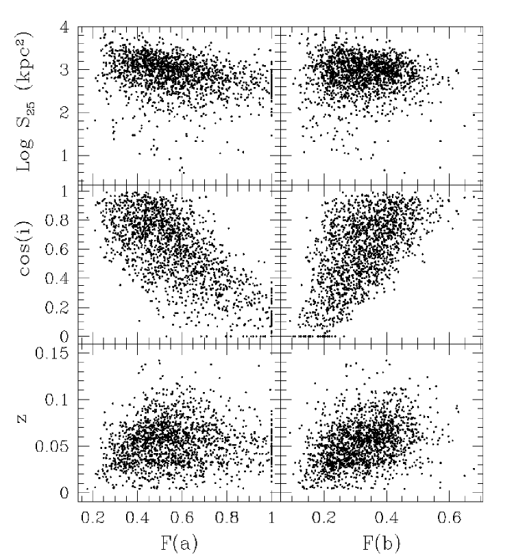
Figure 3. For the whole sample (1671), fractions of the galaxy image covered by the 8″ wide slit if the slit was positioned along the major axis, $F(a)$, or the minor axis, $F(b)$, as a function of the physical size at 25 mag arcsec^-2, $S_{25}$ (upper panels), the cosine inclination angle, cos($i$) (middle panels), and the redshift, $z$ (lower panels).

as a function of $S_{25}$, defined as the rest-frame projected area brighter than $b_{J}=$ 25 mag arcsec^-2 in kpc², and of the galaxy inclination $i$, defined by $\sin^{2}(i)=[1-(b/a)^{2}]/0.96$ [1926] (Fig. 3). For the second possibility we calculated $F(b)$, using the same approximation with $8a$ replaced by $8b$. The true configuration must lie between these two possible extremes. With an 8″ wide slit, this fraction depends mainly on the galaxy inclination, $i$, rather than on $S_{25}$ (Table 1). As seen in Figure 3, our typical spectrum samples the light from $\sim 45\%$ of the rest-frame projected area of the galaxy. The Figure and Table show also that $F(a)$ and $F(b)$ are respectively 2% and 7% larger at $z>0.05$ than at $z<0.05$. Thus the average fraction of galaxy projected area covered by our slit does not depend strongly on redshift; the high-$z$ galaxies have only 5% more coverage than the low-$z$ ones.

Figure 4 shows that $\cos(i)$ and $S_{25}$ are barely correlated, which demonstrates that the SAPM survey is representative of the different kinds of nearby galaxies at $15\leq b_{J}\leq 17.15$. A galaxy sample with random inclinations would have a uniform distribution as a function of $\cos(i)$, but our sample is biased towards galaxies with low inclination angles, as expected in magnitude-limited surveys [1995]. This is because the more inclined a galaxy is, the more its intrinsic galactic absorption reduces the light along the line of sight. Thus with the same absolute luminosity and distance, an inclined galaxy is likely to be fainter than a face-on galaxy. This effect will be particularly strong in blue-selected surveys where dust absorption is large.

3 ELG fraction

3.1 Classification of spectra

We classified spectra according to the H$\alpha$ recombination line; when it is detected in emission as an emission-line galaxy (ELG), otherwise as a non emission-line galaxy (non-ELG). The level of detection of H$\alpha$ depends on the intensity of the line, on its equivalent width, and on the signal-to-noise of the continuum. Thus when comparing the ELG fraction to other surveys, one has to bear in mind the limits of detection of emission lines. Another point is that H$\alpha$ may suffer from stellar absorption, reducing the EW of emission by as much as 5 Å (see Kennicutt 1992), especially in the case of early-type galaxies. Weak H$\alpha$ lines ($\ll 10$ Å) may not be detected, which would lead to a non-ELG classification.

An ELG classification scheme based on H$\alpha$ has the following advantages: (a) Comparison of H$\alpha$ to [N II], [S II] and [O I] allows discrimination between AGN and H II galaxies [1987]. (b) It is a tracer of recent star formation for most galaxies [1992]. (c) Of the Balmer lines, it is the most directly proportional to the ionizing stellar UV flux at $\lambda<912$ Å (see Osterbrock 1989 for a review; Schaerer & de Koter 1997 for recent models), because the weaker Balmer lines are much more affected by the equivalent absorption lines produced in stellar atmospheres. (d) It does not depend strongly on the metallicity, which is not the case for the other commonly observed optical lines such as [N II], [S II], [O II] and [O III]. Since these latter are forbidden lines, their presence depends also on the density of the gas. They have higher ionizing potential than Balmer lines, thus depend also on the hardness of the ionizing stellar spectra. (e) It is less affected by dust than any other lines at shorter wavelengths. Consequently a classification based on H$\alpha$ has the advantage that it is more or less comparable at any redshift with less dependence on chemical evolution than other spectral features.

When H$\alpha$ falls in the wavelength coverage gap $\sim$7000–7020 Å (see Section 2.1), we cannot see whether this line is in emission or not. To avoid introducing any bias, we systematically did not classify these spectra, even if other lines strongly suggest that H$\alpha$ should indeed be in emission or absorption. There are 82 spectra in this category, which represent $5\%$ of the sample of 1671 spectra. 990 ($59\%$) spectra have been classified as H$\alpha$ emitters, i.e. as ELG, and 599 ($36\%$) as non-H$\alpha$ emitters, i.e. as non-ELG. If we assume that the 82 unclassified spectra are distributed like the classified ones, this give $62\%$ of ELG with EW(H$\alpha$) $\ga 2$ Å, and $38\%$ of non-ELG. However the red gap location means that these unclassified galaxies are mainly at $z\sim 0.06$ (see Fig. 7), and thus they are mainly bright (M($b_{J}$)$<-$21 in Fig. 8) where, as we will see, the fraction of ELG is smaller than at fainter magnitudes. When we do attempt to classify the 82 spectra by taking into account the presence of other spectral lines, we find the percentage of ELG and non-ELG is $61\%$ and $39\%$. This is essentially the same as assuming that the 82 spectra are distributed like the classified ones, and so we conclude that any bias due to H$\alpha$ falling in the wavelength coverage gap is insignificant.

3.2 ELG fraction and slit effects

Since the SAPM spectra are not integrated over the whole galaxy, the fraction of ELG with EW(H$\alpha$) $\ga 2$ Å may be slightly higher than estimated in Section 3.1. Indeed, one strong H II region outside the central galaxy region can change an absorption-like spectrum into an ELG. Thus if the 8″ wide slit did not cover this H II region, a galaxy would be classified as non-ELG rather than ELG.

However, since the spectral slit covers on average 45–50% of the galaxy, and since H II regions are mainly distributed along the spiral arms, our fraction of ELG should remain approximately correct. Even though the distribution of H II regions tends to be more centrally concentrated in bulge dominated systems, the luminous H II regions tend to be found at larger radius in late-type spirals (see for instance Hodge & Kennicutt 1983). No bias should arise for galaxies with central H$\alpha$ emission. The major caveat might come from irregular systems where star-forming regions can be found anywhere. In the SAPM sample, galaxies classified as irregular represent only 5%. The morphologically unclassified galaxies (21%; see Table 1 in Loveday, Tresse & Maddox 1999) typically have small images with no easily identifiable morphological features. They are likely to be early Hubble-type galaxies, or spirals with weak spiral arms, or compact galaxies, and are very unlikely to be irregulars. Those galaxies with only one dominant H II region in the disk (perhaps due to an interaction with another galaxy for instance), should represent a very small fraction. In these cases, there was $\sim 50\%$ chance for having observed the H II region with an 8″ slit. Moreover, we note that 50 spectra were re-observed because there were no obvious spectral features to identify accurately a redshift; these re-observed spectra still remain non-ELG, even though the slit orientation changed. Moreover in Section 3.4, we find that very few non-ELG (11) have a 4000 Å break consistent with what is expected for blue galaxies, hence it tells us that our fraction of ELG should be correct to 1%.

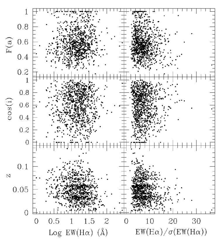
Figure 5. Log EW(H$\alpha$), and detection level of EW(H$\alpha$) as a function of the fraction of the galaxy image covered if the slit was positioned along the major axis, $F(a)$ (upper panels), the cosine inclination angle, cos($i$) (middle panels), and the redshift, $z$ (lower panels).

Figure 5 shows that neither EW(H$\alpha$) $\ga 2$ Å nor the signal-to-noise of the measurements depend globally on the galaxy inclination angle, $i$, or the fraction of area covered by the 8″ slit. Consequently we find that the SAPM sample shows no trend to detect more ELG than non-ELG as a function of inclination angles $i$ (Fig. 4). The means of the axial ratios, ($b/a$), are similar for ELG and non-ELG, respectively 0.60 (or $i=55\degr$) and 0.63 (or $i=52\degr$).

3.3 Correlation of the ELG fraction with galaxy properties

The average parameters ($b_{J}$, $z$, $kz$, $M(b_{J})$, $\mu_{25}$, $S_{25}$) for the SAPM galaxies are summarized in Table 2. The fraction of ELG does not globally depend on $b_{J}$ (Fig. 6), showing that the EW is not dependent on apparent magnitude. This is because the integration times were adjusted for each galaxy (see Section 2.1). Figure 7 shows that the ELG fraction does not systematically depend on redshift, but there is a slight excess at $z<0.014$; we discuss this later.

The ELG fraction depends strongly on the absolute magnitudes (Fig. 8); from $M(b_{J})=-23$ to $-18$ mag, it increases by a factor of 2. The fraction also depends on the physical size of galaxies (Fig. 9); from $S_{25}=10000$ to $100$ kpc², it increases by a factor of 4. ELG are more common than non-ELG in intrinsically faint galaxies, and small systems. ELG are on average $0.43\pm 0.06$ mag fainter than non-ELG. If we exclude galaxies at $z<0.014$ (see below), ELG are $0.33\pm 0.05$ mag fainter than non-ELG. The apparent flattening of these trends at $M(b_{J})>-18$ and at $S_{25}<40$ is probably due to the combination of the small number of galaxies in these bins, and the fractions approaching $100\%$.

The dependence on rest-frame surface brightness averaged over the area brighter than $b_{J}=25$ mag arcsec^-2, $\mu_{25}$, is more complex. The fraction of ELG decreases by a factor 2 from $\mu_{25}=21.9$ to 23.1 mag arcsec^-2, and increases by the same factor towards fainter values (Fig. 10). Galaxies with $\mu_{25}>24$ are at $z<0.014$. ELG are more common for the highest and lowest surface brightness galaxies than non-ELG. This means that faint, small systems which contribute most to the ELG sample may be either high-surface brightness, compact galaxies, or low-surface brightness dwarfs.

Going back to the ELG fraction as a function of $z$ we can now understand the high fraction at $z<0.014$. The SAPM sample is magnitude-limited with both high and low magnitude limits, and so at $z<0.014$ we observe only small, $M(b_{J})>-18$ galaxies. From Figure 8, we see that most galaxies this faint are ELG, so we expect to see a high ELG fraction at these low redshifts.

To summarize, ELG galaxies are found more frequently at fainter intrinsic magnitudes, and in smaller systems than non-ELG. This agrees with the general picture where dwarf and compact galaxies are more actively forming stars than their bright counterparts in the local Universe. This is a reflection of the difference between ELG and non-ELG luminosity functions [1999]. It is also consistent with the rapidly evolving population of small galaxies up to $z\sim 1$ [1998]. The overall blue luminosity density is dominated by bright galaxies, which formed most of their stars much earlier than dwarfs, which are actively forming stars today.

3.4 Correlation of the ELG fraction with D₄₀₀₀

We estimated the 4000 Å break using the D₄₀₀₀ index as defined in Section 2.2. The measured values of D₄₀₀₀ range from 0.9 to 2.5, with a mean of 1.6. These values are consistent with the limits obtained with spectral evolution of stellar populations using isochrone synthesis. For instance in Fig. 13b (D₄₀₀₀ versus age, assuming solar metallicity) of Bruzual & Charlot [1993], this index never reaches values above 1.5 if a constant star formation rate is adopted, while a $10^{8.5}$ year old instantaneous-burst or a $10^{9.5}$ year old 1Gyr-burst reproduce these high values. Thus half of the local population is dominated by star bursting of at least $10^{8.5}$ year old. The other half is dominated by younger star formation whatever the star formation rates adopted.

The D₄₀₀₀ distribution for ELG is clearly different from the non-ELG distribution (Fig. 11), the average D₄₀₀₀ for ELG is $31\%$ smaller than for non-ELG (see Table 2). However, there is an overlap between the two distributions, and there is no clear separation into distinct populations. The presence of H$\alpha$ in emission is correlated with a low D₄₀₀₀, which is expected since both are indicators of massive star formation. It strengthens the link between our H$\alpha$ ELG classification and star formation activity. In general, the smaller D₄₀₀₀, the bluer the galaxy color; as expected our ELG have bluer colors on average than the non-ELG.

We note that $1\%$ (12) of ELG galaxies have $D_{4000}>2$, the value characteristic of elliptical galaxies. They are bright galaxies ($M(b_{J})\leq-21.6$), and have EW(H$\alpha$) $\simeq$ EW([O II]) $\simeq 8$ Å. In these systems, stellar absorption at H$\alpha$ must be significant, and thus their true EW(H$\alpha$) must be higher, as we expect from the relation between [O II] and H$\alpha$ (see Section 7.1). These galaxies have a significant old stellar population, and are undergoing current star formation; most of them have a spiral morphology.

Also $2\%$ (11) of non-ELG have $D_{4000}<1.2$, the value typical of very blue galaxies. They span the whole range of luminosities, they have no [O II] line. Five are spirals, two are ellipticals, one is irregular and three are not morphologically classified. For some of them, this could be due to slit effects as discussed in Section 3.2.

Figure 12 shows that nearly all galaxies fainter than $M(b_{J})=-19$ have $D_{4000}<1.7$. Most dwarf galaxies tend to have rather young stellar populations, consistent with the high fraction of ELG that we find at faint magnitudes.

4 Comparison of the ELG fraction with other surveys

Comparing average properties from different surveys is never a straightforward task. Different detection limits, different instrumentation, different criteria for galaxy selection and different methods of classifications must be taken into consideration otherwise results of the comparison may be very misleading.

4.1 The CFRS-12 sample ($\mn@boldsymbol{\mathbf{0.1}<z<\mathbf{0.3}}$)

The CFRS-12 sample [1996] is magnitude limited in the same way as the SAPM, and has $\langle z\rangle=0.2$. Galaxies in CFRS-12 were selected on $I$ magnitude (i.e. more sensitive to old stellar populations), while the SAPM used $b_{J}$ selection (i.e. more sensitive to star forming galaxies). The galaxy area covered by the 1$\aas@@fstack{\prime\prime}$75 CFRS slit for galaxies at $z\simeq 0.2$ is similar to the 8″ SAPM slit for galaxies at $z\simeq 0.05$ (i.e. $\sim 50\%$ of the galaxy area).

In CFRS-12, $85\%$ of the galaxies are H$\alpha$ emitters with EW(H$\alpha$ + [N II]) $\ga 10$ Å  and $-21.5<M(B_{AB})<-14$ (see Table 1; Fig. 14 of Tresse et al. 1996). In Figure 13, CFRS-12 galaxies follow the same trend as SAPM galaxies in Figure 8; a higher fraction of ELG is found at fainter blue absolute magnitudes. Similarly to the SAPM, in the CFRS-12, the non-ELG population is brighter by $\sim 1$ mag, and redder by $\sim 0.4$ mag than the ELG population.

To make a fair comparison between the two surveys, we limit the samples to EW(H$\alpha$ + [N II]) $\geq 10$ Å for ELG, and $-17\leq M(B_{AB}\simeq b_{J})\leq-21$. We obtain $82\%$ and $65\%$ of ELG respectively for these subsets of the CFRS-12 and SAPM samples. Thus even though SAPM galaxies were selected from their rest-frame blue continuum, and CFRS-12 galaxies from their rest-frame red continuum, the fraction of ELG at $z=0.2$ is higher by a factor 1.3 than locally. The exclusion of APM merged systems ($<3\%$, see Section 2) would not change this result. Moreover the APM galaxy catalog is known to miss $\sim 5\%$ of compact galaxies which are difficult to distinguish from stars (see Maddox et al. 1990); even if this fraction is as much as $10\%$, the fractions of ELG for the same EW limit at low and high redshifts would still be discrepant.

This result is consistent with the rapid evolution in H$\alpha$ luminosity density [1998]. On average at higher redshifts H$\alpha$ is more intense, and consequently for the same EW limit, the fraction of ELG increases. An important point to note is that the ELG fraction does not depend on the relative normalization of the galaxy counts, and so this result is an independent demonstration of rapid galaxy evolution at relatively low redshifts ($z<0.3$).

4.2 Other surveys

Statistically complete, magnitude-selected spectroscopic surveys which have H$\alpha$ line information are rare. In the very nearby Universe ($z\ll 0.005$), Ho et al. [1997b] spectroscopically observed 486 galaxies from the Revised Shapley–Ames Catalog of bright galaxies ($B_{T}\leq 12.5$ mag) which contains all morphological types. Only the central few hundred parsecs of the galaxies have been observed with a 2″ x 4″ slit, but the detection limit of emission lines is very low, at EW $\sim 0.25$ Å ($3\sigma$). After removing the stellar background of the bulge, and thus correcting for stellar absorption (which does not exceed 2–3 Å, Ho et al. 1997a), they detected optical line emission in $86\%$ of the galaxy nuclei. Their result implies that ionized gas is almost invariably present in the core of galaxies. From Ho et al. [1997b] figures 4 and 6, we estimate that $\sim$60–65% of the emission-line nucleus galaxies (ELNG) within roughly the same absolute $B$-magnitude range as SAPM, have EW(H$\alpha$) $>2$ Å. This fraction is similar to that found by Véron–Cetty & Véron [1986] (60–65%), who did not subtract the stellar background. The differences in apertures and signal-to-noise mean we cannot directly compare this fraction to the SAPM or the CFRS-12 samples, however we will make one comment.

The SAPM 61–62% ELG fraction is close to the $\sim$60–65% ELNG. Since $\sim$40–50% of the galaxy area is surveyed in the SAPM galaxies, this suggests that H$\alpha$ emission from the disk causes little change in the number of H$\alpha$ emitters detected above 2 Å. Overall, the nuclear emission amounts to a few percent of the integrated flux (see Kennicutt & Kent 1983), so we might have expected more H$\alpha$ emitters in the case of the SAPM in which the extra-nuclear emission is observed. This is not the case, because the extra-nuclear nebular emission varies roughly in proportion to the continuum, and thus the EW is relatively unchanged. This is consistent with detailed studies by Hunter et al. [1998] who show that in irregular galaxies, the star formation rate (measured from H$\alpha$ luminosities) and the total stellar density (measured from the surface brightness) lie close to each other throughout the whole galaxy, and by Ryder & Dopita [1994] who observed that the star formation follows the old stellar mass surface density in spiral galaxies. For the surface brightness profiles of typical SAPM galaxies, this implies that the detected H$\alpha$ emission is centrally peaked for most of the SAPM ELG. This is seen also in other surveys which select only emission-line galaxies, such as the UCM survey [1998]; these find that the line emission comes largely from the nuclear region.

5 Emission-line and continuum properties

We investigate in this section how H$\alpha$, [N II], [S II], [O II] and [O I] correlate with $b_{J}$ luminosity, and D₄₀₀₀.

5.1 H$\alpha$ and M($b_{J}$)

Out of the 990 ELGs, 56 ($6\%$) have detectable H$\alpha$ emission that could not be properly measured, usually because it was at the same wavelength as a sky line. For the remaining 934 ELG, $98\%$ have EW(H$\alpha$) under 60 Å, (20 have EW $>60$ Å). The mean and median EW(H$\alpha$) ($>2$ Å) are respectively 19 and 15 Å.

Figure 15 shows that the fraction of faint ELG ($M(b_{J})>-21$), increases as a function of EW. From EW(H$\alpha$) $=10$ to 60 Å, the fraction increases by a factor $\sim 2$. Another way to look at this is to consider the fraction of high EW ELG (EW$>15$ Å), which increases at fainter M($b_{J}$) (see Fig. 14).

These trends are the continuation of those seen for the ELG fraction as a function of M($b_{J}$), and they reflect a global tendency within the whole population; the larger EW(H$\alpha$), the bluer the galaxy (Kennicutt & Kent 1983). This is because EW(H$\alpha$) is the ratio of the flux originating from UV photionization photons ($<912$ Å), over the flux from the old stellar population emitted in the rest-frame R passband, which forms the continuum at H$\alpha$. Thus large EW is either due to a large UV flux (or $B$ absolute magnitude since they are correlated), or to a small continuum from the old stars. In either case this implies a blue continuum colour. Hence the observed trend of larger EW(H$\alpha$) for fainter galaxies implies that the faint ELG population is dominated by blue galaxies, while the bright ELG population is dominated by redder galaxies.

So, the galaxies which evolve rapidly with redshift (at least up to $z=1$) are faint and dominated by a young stellar population. The bright galaxies evolve more or less passively and are dominated by an older stellar population. It is now well established that the faint end of the luminosity function of $B$-selected galaxies is dominated by actively star-forming galaxies. This is what we find also in the SAPM [1999].

Since $B$-luminosity is strongly correlated with H$\alpha$ luminosity [1998], the fainter a galaxy, the smaller its H$\alpha$ luminosity is, and thus the faint population does not dominate the total H$\alpha$ flux density, or the UV ($<912$ Å) ionizing flux density at low $z$, even though it is the population which evolves most rapidly with redshift.

5.2 [N II], [S II], [O II], [O I] detection and M($b_{J}$)

In this subsection, we discuss measurements of [N II] $\lambda$6583, [S II] $\lambda\lambda$6716, 6731, [O II] $\lambda$3727 and [O I] $\lambda$6300 for the 934 H$\alpha$ ELG with quantified EW(H$\alpha$). [N II] $\lambda$6548, which is 3 times fainter than [N II] $\lambda$6583, has often too low signal-to-noise to be detected in the same homegeneous way as its counterpart at 6583 Å.

We measured [N II] for 784 galaxies ($84\%$). The average EW([N II]) detection is at $4.7\sigma$, which is $\sim 19\%$ lower than the one for H$\alpha$. Since the wavelengths are very close, the difference is because on average [N II] has smaller intensity. This is to be expected since [N II] is harder to ionize, and less abundant than H$\alpha$. The remaining [N II] are 46 ($5\%$) with no detection above $\sim 2$ Å, 43 ($5\%$) detected but too noisy to be measured, 31 ($3\%$) with a sky subtraction problem, and 30 ($3\%$) not observed because it falls in the gap at 7000–7020 Å (see Section 2.1).

We measured [S II] $\lambda\lambda$6716, 6731 for 506 galaxies ($54\%$); for 30 ($3\%$) galaxies only one line could be measured. In these cases the other line has a too low signal-to-noise to be reliably measured, and we set the EW to zero. The average EW([S II] $\lambda\lambda$6716, 6731) detection for these 536 galaxies is at $4.3\sigma$, which is $\sim 30\%$ lower than H$\alpha$. This is partly because [S II] has a smaller intensity than H$\alpha$ (as in the case of [N II]), but also because the continuum at 6717–6731 Å is more noisy than at H$\alpha$; sky lines start to increase the noise in the red continuum. For 123 galaxies no line was detected, and for the remaining 275 galaxies, one of the lines was either on a sky line or in the gap. The percentage of [S II] detected above 2 Å is higher than for [N II], because the sum has higher intensity, even though individual lines are harder to detect.

We measured [O I] $\lambda$6300 for 43 galaxies (3%). The average detection of EW[O I] is 2.7$\sigma$, it is the lowest value since this line intensity is usually extremely weak relatively to the other lines.

We measured [O II] for 859 galaxies ($92\%$). The average detection is $4.8\sigma$, which is $\sim 15\%$ lower than for EW(H$\alpha$). This is because the blue continuum is less intense than the red continuum, and consequently more noisy. We find 75 galaxies with significant H$\alpha$ but no detectable [O II]. The EW(H$\alpha$) for these galaxies is detected at more than $3\sigma$, and lies in the range 2–24 Å, with a mean at 8 Å. They have also $1.3<D_{4000}<1.8$, and a median $D_{4000}=1.5$. Out of the 75, 58 have [N II] detected, and 15 have also [S II] detected. These galaxies are undergoing star bursts, and are probably heavily absorbed so that they show a moderate Balmer break, and a weak noisy blue continuum (see also Section 8). They are not preferentially edge-on galaxies.

Figure 15 shows that the fraction of faint galaxies ($M(b_{J})>-21$) increases as a function of: (a) [N II] EW by a factor 1.2 from 2 to 15 Å, (b) [S II] EW by a factor 2 from 2 to 20 Å, and (c) [O II] EW by a factor 2 from 2 to 40 Å. These trends are analogous to what we see for H$\alpha$, where the fraction of faint ELG increases by a factor 2 up to EW(H$\alpha$) $=60$ Å. Faint galaxies have larger EW for emission lines both in the blue and red band at rest. Thus, as well as being bluer as seen previously, they have also stronger photoionization sources which enhance forbidden line intensities. Indeed, if there was simply a larger amount of young stellar background in the blue, then EW([O II]) would decrease while EW([S II]) would increase, (noting that [O II] has similar photoionization conditions to [S II]). So, the enhancement of UV photoionization sources is coupled with a larger amount of $B$-band flux produced mainly by intermediate-mass stars. This leads to the correlation between H$\alpha$ and $B$ luminosity [1998]. These metallic lines follow the same trend as H$\alpha$, suggesting that they have a common source of ionization. The small number of galaxies with detected [O I] makes the comparison more difficult, however the fraction of faint galaxies seems not to be correlated with this weak line. Emission-line ratios are studied in the following Section, and correlations are studied in Section 7.

The medians of the EW distributions for the bright and faint ELG populations are listed in Table 3. The difference between these medians is largest for [O II] (47%), then H$\alpha$ and [S II] ($\sim 31$%). We can interpret these variations as follows: EW([O II]) is the most sensitive to blue luminosity, since it depends directly on the rest-frame $B$-band continuum; EW(H$\alpha$) and EW([S II]) are slightly less sensitive since they depend on the rest-frame $R$-band continuum.

For [N II] there is no significant difference (4% discrepancy). The global behavior of EW([N II]) reflects intrinsic differences in the nitrogen abundance (N/O) in ELG. The origin of nitrogen is still an open debate (see for instance data analysis in Izotov & Thuan [1999], Garnett [1990], Kobulnicky & Skillman [1998] and references within). On one hand, the nature of stars producing the primary nitrogen (i.e. from burning H and He via fresh C and O) remains unclear in low-metallicity systems (high- or intermediate-mass stars). On the other hand, the scenario to explain a second source for nitrogen enrichment observed in high-metallicity galaxies is still open. We cannot address these points in detail here. However in our representative local sample, we find that on average luminous blue ELG are likely to be enhanced in nitrogen abundance. This suggests that in faint, low-mass, late-type ELG, nitrogen is a primary element, whereas in more bright, more massive galaxies nitrogen it comes from a secondary source. Thus the expected global increase in the fraction of faint galaxies as a function of line strengths would not be observed in the case nitrogen enhanced in a non negligible fraction of bright galaxies.

5.3 Emission-line EW and D₄₀₀₀

As seen in Section 3 the presence of H$\alpha$ in emission is correlated with a low D₄₀₀₀ index. This trend continues within the ELG population; the larger is EW(H$\alpha$), the smaller is D₄₀₀₀.

Figure 16 shows that the fraction of ELG with low D₄₀₀₀ ($<1.4$) increases as a function of: (a) H$\alpha$ EW by a factor 4.5 from 2 to 60 Å, (b) [O II] EW by a factor 3.4 from 2 to 40 Å, (c) [S II] EW by a factor 4.6 from 2 to 20 Å, (d) [N II] EW by a factor 2 from 2 to 15 Å. The medians of the EW distributions for the low and high D₄₀₀₀ ELG populations are listed in Table 3. They are the most discrepant for H$\alpha$ (69%), then [O II] (52%), [O I] (40%), [S II] (36%), and [N II] (35%). EW(H$\alpha$) is the most sensitive to D₄₀₀₀ as expected, since these two measurements are the most sensitive tracers of star formation rate. Here [N II] and [O I] follow the same trend as for the other lines, in contrast to their behavior as a function of rest-frame blue luminosity. This is because a low D₄₀₀₀ is caused by the high-mass stars which enhance all line strengths.

6 Emission-line ratios

6.1 [N II]/H$\alpha$, [S II]/H$\alpha$, [O I]/H$\alpha$ ratios

The ratio [N II] $\lambda$6583/H$\alpha$ involves lines close in wavelength, and thus it does not depend on reddening or flux calibration. The EW ratio must be in principle equivalent to the flux ratio, since the continuum is the same. It is a good ratio to compare galaxies at different redshifts.

Only substantial stellar absorption at H$\alpha$ may affect this comparison: in late-type galaxies, it is usually negligible; it may become significant in early types, which exhibit Balmer absorption lines. For SAPM galaxies where [N II] is detected, it is certainly negligible. Indeed only detailed studies with a level of detection lower than 2 Å EW can detect weak [N II] in early-type galaxies [1997a].

Figure 17 shows the distribution of the [N II]/H$\alpha$ EW ratios for our 784 galaxies with EW(H$\alpha$) + 1.33EW([N II] $\lambda$6583) $>3$ Å. We note that the ratio does not show any trend with redshift. The median and mean values are 0.37 and 0.41, and we find much the same values using our relative flux ratios, 0.36 and 0.40. We also show the distribution of the ratios published by Kennicutt (1992, hereafter K92) in his tables 1 & 2 respectively of high (5–7 Å) and low ($>10$ Å) resolution spectra. We excluded the H ii regions (Mkr 59 and Mkr 71), the Seyfert 1 galaxies (NCG 3516, NGC 5548 and NGC 7469) and galaxies with EW(H$\alpha$) + EW([N II] $\lambda\lambda$6748, 6583) $<3$ Å as in the SAPM. We note that his table 2 contains galaxies already tabulated in table 1. For these, we used the measurements from his table 1. In total, K92’s sample has 57 ratios of narrow-line fluxes integrated over the whole galaxies. Since the K92 galaxies are not a complete magnitude-limited sample, it is dangerous to consider the observed distributions of any parameter as representative of the true distributions. Therefore we calculated the distribution of the [N II]/H$\alpha$ EW ratios separately for each morphological type, and averaged them with weights proportional to the fraction of each type in the RSA (Sandage & Tammann 1981). The median and mean ratios are 0.38 and 0.47 for this K92 sample.

The median and mean ratios for the SAPM and K92 samples are similar. Kennicutt’s values are slightly higher because his ratios are likely to be biased towards higher values, as discussed in K92. This tells us that the SAPM spectral properties are on average well representative of integrated spectra (see also Fig. 25). As noted by K92, undersampling the disk tends to reduce the strengths of the emission lines in roughly equal proportion, and thus the relative line fluxes should be insensitive to it. This strengthens our conclusions from Section 2, showing that our results are very unlikely to be affected or biased by using a long slit.

The median and mean for the EW ratio, [S II] $\lambda\lambda$ 6716, 6731/H$\alpha$, are 0.36 and 0.42, and for the flux ratio, are 0.36 and 0.41. If we take only our spectra for which [S II] lines fall on the same CCD chip as H$\alpha$, we have similar values, respectively 0.37 and 0.43, 0.36 and 0.41. This tells us that the relative calibration for the continuum of the two red chips is on average good to about $1\%$. The median and mean for the EW ratio, [O I] $\lambda$ 6300/H$\alpha$, are 0.08 and 0.11, and for the flux ratio, are 0.08 and 0.42. The fact that the EW and flux ratio averages are similar shows that the red continuum at H$\alpha$ and at [S II] or [O I] is not significantly different.

[N II]/H$\alpha$, [S II]/H$\alpha$ and [O I]/H$\alpha$ (Fig. 17) are commonly used to distinguish galaxies hosting an AGN from the others. We analyse them elsewhere.

6.2 [N II]/H$\alpha$ versus EW(H$\alpha$ + [N II])

In deep optical surveys, H$\alpha$ and [N II] $\lambda\lambda$6548, 6583 lines are often blended because of the use of low-resolution spectroscopy. It is however important to recover the flux solely in H$\alpha$ to measure for instance the H$\alpha$ luminosity function, hence to derive a star formation rate. This is also necessary to distinguish AGN galaxies from H II galaxies, in particular in narrow-line emission galaxies. Broad-line galaxies are identified straightforwardly as AGN, and they are not numerous in representative surveys of field galaxies.

The value of the ratio [N II] $\lambda\lambda$6548, 6583/H$\alpha$ is usually taken to be 0.5 to remove the contribution of [N II] to (H$\alpha$ + [N II]) blended emission, as determined by Kennicutt [1992]. Using the SAPM sample, we study this ratio in more detail. We note that including AGN changes the average values very little, since the overall emission is dominated by stellar emission in local representative surveys.

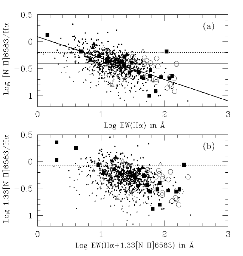
Figure 18. (a) Log [N II] $\lambda$6583/H$\alpha$ versus Log EW(H$\alpha$). (b) Log 1.33 [N II] $\lambda$6583/H$\alpha$ versus Log EW(H$\alpha$) + 1.33EW([N II] $\lambda$6583). Dots are SAPM ($>3\sigma$) data, crosses are SAPM ($<3\sigma$) data. Open symbols are K92 high-resolution data, filled symbols are K92 low-resolution data. Triangles are AGN and circles are normal galaxies in K92 sample. The dotted line is the empirical separation between AGN and H ii galaxies. The solid line is the commonly used average value for [N II]/H$\alpha$. The diagonal line is our best fit to the correlation.

Figure 18a shows that [N II] $\lambda$6583/H$\alpha$ EW ratio decreases as a function of EW(H$\alpha$). In this plot we consider only spectra with [N ii] EW detected above $3\sigma$. We fitted a least square relation to the log of the data ($\log$[N II]/H$\alpha=-0.4\log$EW(H$\alpha$) $+0.1$). At our median EW(H$\alpha$), the relation gives a [N II]/H$\alpha$ ratio of 0.4, i.e. 0.5 for ([N II] $\lambda\lambda$6548, 6583)/H$\alpha$. We recall that 1.33 [N II] $\lambda$6583 should be equivalent to [N II] $\lambda\lambda$6548, 6583 since [N II] $\lambda$6548/[N II] $\lambda$6583 $=1/3$. In this figure, we also plot K92’s sample; we see that the high-resolution K92 subsample is generally above our SAPM trend because it contains a large fraction of early-type galaxies which have systematically higher ratios. The low resolution K92 data are slightly higher than our median value because of K92’s exclusion of weak H$\alpha$ + [N II] blended lines.

Figure 18b shows the relation 1.33 [N II]/H$\alpha$ EW versus EW(H$\alpha$) + 1.33 EW([N II]). The trend is the same as in Fig. 18a. Thus we can predict which value is expected for the ratio when observing the blend H$\alpha$ + [N II]. For instance, if this latter is $\sim 100$ Å, the ratio should be $\sim 0.3$, whilst if it is $\sim 20$ Å, it should be $\sim 0.7$.

In terms of galaxy numbers, the slight overestimation for bright galaxies (mainly low EW), and underestimation for faint galaxies (mainly high EW) are about counterbalanced, since 0.5 is the median value. In fact, as we will see in Section 7, our relations [O II]–H$\alpha$ and [O II]–(H$\alpha$ + [N II]) are equivalent if this median is taken. However this argument applies only for a similar EW(H$\alpha$) distribution. Samples at higher redshifts are skewed towards higher EW compared to the local samples (at least in [O II] EW, see Fig. 25), and thus the local median, $0.5$, is not the correct one to use. This effect will be more significant in small samples at high redshift.

7 Correlation between emission lines

7.1 [N II], [S II], [O II], [O I] versus H$\alpha$

Figs. 19,  20,  21 &  23 show that EW of [N II] $\lambda$6583, [S II] $\lambda\lambda$6716, 6731, [O II] $\lambda$3727, [O I] $\lambda$6300 increase as a function of H$\alpha$ EW. The figures are on a log-log scale to show all points, in particular those with low EWs. We note that this scale enhances the dispersion of low EWs in comparison with the one of high EWs. Table 4 gives the correlation parameters. The correlations are measured with EW, and not log(EW).

The large scatter (rms of about $50\%$) found in the EW correlations is not due to poor signal-to-noise; the scatter is still large even with lines detected above $5\sigma$. In the case of [N II] or [S II] lines, it is independent of the red stellar background. It simply reflects real scatter in the main physical parameters (metallicity, effective temperature, ionisation parameter) which drive variations in the strengths of various forbidden transitions relative to the recombination lines. In addition, any presence of AGN, in particular in early Hubble types, and any contribution to the emission from the diffused ionized gas will increase the primary scatter (see for instance [1997c] and references within). The dispersion is larger for the [O II] correlation. In this case, the effect is accentuated by the diversity of young stellar contents which produce the continuum at [O II]. Although the [O I] line is rarely detectable, we were able to measure the EW in a few galaxies. For this line the dispersion is as large as $\sim$80%. The scatter is so large partly because of the weakness of the line intensity which leads to low signal-to-noise, and partly because most of the [O I] flux comes from the partially ionized transition zone produced by high-energy photoionisation, which means the [O I]/H$\alpha$ ratio is very sensitive to the structure and thickness of the zone. We flagged all objects having [N II] $\lambda$6563/H$\alpha>0.63$ (i.e. as good candidates for hosting an AGN) with starred symbols. Excluding them changes the correlations by less than $5\%$. The fractional dispersions are almost independent of the EW strength. Since EW is correlated with luminosity (see Section 5.1), this implies that both faint and bright galaxies have a variety of photoionization environments.

Since [O II] is at short optical wavelengths and is correlated with H$\alpha$ strength, it has been used as a star formation rate (SFR) indicator for high-$z$ galaxies, when H$\alpha$ is not visible in the optical window at $z>$ 0.3–0.4. From the K92 relation, EW([O II]) $=0.4$ EW(H$\alpha$ + [N II] $\lambda\lambda$6548, 6583), we assumed his quoted value [N II] $\lambda$6583/H$\alpha$ = 0.53, and derived EW([O II]) $\simeq 0.6$ EW(H$\alpha$). Our value is discrepant with K92 by $\sim 10\%$, which is not significant given the dispersion of the data in both samples.

We note that EWs measured from the overall galaxy content are likely to be affected by dust. Indeed, recombination emission lines originate from dusty H II regions where hot stars (OB type) are formed, whereas the continuum at [O II] or H$\alpha$ comes from long-lived stars sitting in less, or non obscured regions. EW([O II]) is more affected by the dust than EW(H$\alpha$). Hence, the intrinsic [O II]–H$\alpha$ EW ratio should be on average slightly larger than our observed relation.

7.2 The [O II]–(H$\alpha$ + [N II]) relation in different surveys

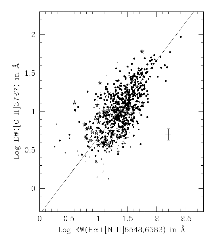
Figure 22. Log EW([O II] $\lambda$3727) versus Log EW(H$\alpha$ + [N II] $\lambda\lambda$6548, 6583). Same notation as Figure 19. EW([O II]) $\approx 0.5$ EW(H$\alpha$ + [N II]) (see Table 4).

The correlation between EW([O II]) and EW(H$\alpha$ + [N II] $\lambda\lambda$6548, 6583) has been commonly used to estimate SFR. In Figure 22, we show it for our SAPM data, and in Figure 24 we plot it together with data from the K92 and CFRS-12 samples. The distribution of K92 data is spread over the SAPM distribution; the correlation and dispersion of K92 data are similar to the SAPM with as little as 5–10% discrepancy (see Table 4). This is just about within the expected random noise; the rms in the mean relation is $\sim 8\%$ for K92, and $\sim$2–3% for the SAPM.

K92 sample has a larger fraction of high EW data. High EWs in K92 sample usually correspond to late Hubble type galaxies (see fig. 11 in Kennicutt 1992). Our median for [O II] and H$\alpha$ + [N II] are about half those for the K92 data. Our EW([O II]) distribution at $z=0.05$ is very similar to nearby samples (see Fig. 25), except for EW $<5$ Å, which is probably due to different detection levels, and magnitude ranges (luminous galaxies of the local Universe usually have low EW). Thus this factor two cannot be due to our undersampling, but rather reflects the difference between a representative sample (SAPM) and a sample selecting specific galaxies (K92).

CFRS-12 data, which is a small representative sample at $\langle z\rangle=0.2$ of galaxies usually fainter than $-21$ in $B$, have stronger EWs. On one hand, the small number of low EW is certainly due to the poor detection of EW lower than 10 Å in the CFRS spectra, and the lack of luminous galaxies at $z<0.3$. On the other hand, the larger fraction of strong EW spectra is genuine, and corresponds to the rapid evolution of faint galaxies, as discussed previously. The distribution of EW in distant surveys such as the CFRS is significantly different than to the local ones (see Fig. 25). Another observation is that the [O II]/(H$\alpha$ + [N II]) ratio for the CFRS-12 galaxies (see Table 4) is $\sim 40\%$ higher than in the local Universe, but the scatter in the data is also larger. The ratio is higher because spectra exhibit stronger [O II] EW than local galaxies with same H$\alpha$ EW. This has been noted by Hammer et al. [1997]. Since the CFRS-12 flux ratio is exactly the same as the CFRS-12 EW ratio, then differences in the color of the continuum do not change the relation. Even strong stellar absorption at H$\alpha$ would not be sufficient to explain the shift towards smaller H$\alpha$ EWs than expected from the local relation at strong [O II] EWs. Therefore the apparent excess of abnormally strong [O II] must correspond to a genuine change in faint galaxies towards higher redshifts, which produces larger degrees of ionization. This suggests that the local relation between [O II] and H$\alpha$ should not be extrapolated to distant galaxies with strong [O II] and very blue continuum, which are more numerous than locally. For these galaxies, the SFR estimated from the [O II] EW and the local relation will be overestimated by as much as $\sim 50\%$. Clearly amongst emission lines, H$\alpha$ is the most reliable tracer of SFR for distant galaxies (see Tresse, Maddox & Loveday 1998).

8 [O II] detected in non-ELG

Out of 599 galaxies with no H$\alpha$ detected, 68 ($11\%$) exhibit [O II] $\lambda$3727. Their distribution is represented in Figure 25; their EW are mainly lower than 10 Å. They are not found at a particular redshift, or magnitude. They have $D_{4000}>1.5$, with a median at 1.8, i.e. these [O II] emitters are lying preferentially in red galaxies. According our relation between H$\alpha$ and [O II], they should have EW(H$\alpha$) $\simeq 15$ Å. Only strong stellar absorption ($>10$ Å) in these red objects would not allow us to detect H$\alpha$. We note that the distribution of their EW([O II]) does not have a preferred galaxy inclination. They are most likely early Hubble type galaxies undergoing modest starbursts. Their morphology is as follows: 10 elliptical, 10 SO, 39 spirals, 1 irregular, and 5 unclassified. They represent only $4\%$ of the total SAPM sample. Analogous objects have been found in the CFRS at $z>0.45$ (see Hammer et al. 1997), i.e. [O II] detected with red colors (H$\alpha$ is not visible). A fraction of $6\%$ (13 out of 210) are detected with an old stellar background. These CFRS galaxies seem to be the equivalent of our non-ELG with [O II] lines detected. It seems that the fraction of such objects increases with redshift, indeed the CFRS has a much lower spectral resolution than the SAPM, which increases the detection limit of [O II], and certainly more [O II] emitters within these early-type galaxies should be found.

Another $5\%$ (10 out of 210) in the CFRS are detected with a young stellar background, but heavily reddened. These galaxies seem more likely to correspond to our galaxies with H$\alpha$ but no [O II] detected (see Section 5.2). In our SAPM spectra, [O II] is not always detected with certainty because the blue continuum is too noisy for these galaxies. In addition, the median of the [O II] EW distribution of local galaxies is lower by a factor $>$2 than the one for high-$z$ distributions, and so EW are expected to be on average smaller (see Table 5). They represent $4\%$ (75 out of 1671) of the total SAPM sample, and thus their fraction seems to be constant with redshift.

If we classify the SAPM galaxies according their [O II] emission, then we find $\sim 61$% of [O II] emitters, which is the same fraction as H$\alpha$ emitters. Indeed galaxies with [O II] but no H$\alpha$ are counterbalanced by galaxies with H$\alpha$ and no [O II].

9 Conclusion

In this paper we have analysed various line EWs and the 4000 Å Balmer break of galaxies in the SAPM survey. This survey uniformly samples all galaxy types, and the spectral properties are representative of the local Universe at $z\sim 0.05$. We would like to point out in particular that our results are independent of any incompleteness in the SAPM morphological classifications and uncertainties in the SAPM flux calibration. Thus our results can on average be compared with deeper surveys. Our main results are:

1. $61\pm 1\%$ of the SAPM galaxies are H$\alpha$-emitters (ELG) with EW(H$\alpha$) $\ga 2$ Å. The detection of H$\alpha$ in emission indicates the presence of newly-formed, short-lived stars ($t<$ few $10^{6}$ yr) which radiate at $\lambda<912$ Å. The ELG fraction increases as the galaxy is fainter and physically smaller. This fraction is larger in high and low surface brightness galaxies, i.e. in compact and dwarf galaxies. ELG have low 4000 Å Balmer breaks, i.e. consistent with massive star formation. Faint ($L<L^{*}_{B}$) galaxies are bluer, and have stronger photoionization sources than bright galaxies. This agrees with the general picture where faint and small galaxies are more actively forming stars than their bright counterparts in the local Universe. This is reflected in the difference between ELG and non-ELG luminosity functions [1999]. It is also consistent with a “peak” in the SFR history since the overall luminosity density is dominated by bright galaxies, which formed most of their stars much earlier than faint galaxies, which are actively forming stars today. The population of small, less massive systems is what evolves rapidly, and undergoes rapid brightening towards earlier epochs.
   

2. Comparison of the ELG fraction with the CFRS-12 sample ($\langle z\rangle=0.2$) demonstrates a rapid evolution of the faint galaxy population at low redshifts. This observation does not depend on the relative normalization of the galaxy counts. Emission lines trace the massive, young, short-lived star galaxy contents, and thus their evolution is more rapid than color evolution. However, since the SFR follows the total stellar or gas density, no strong change in the average spectral properties should be detected, unless some process rapidly enhances the SFR. Except in the case of interacting galaxies, where disruption of the galaxy density will provide a good site for starbursting, for the remaining population, other factors must be taken into account.
   

3. We note a continuity in the spectral properties and luminosities of ELG and non-ELG, and of strong and weak H$\alpha$ emitters. In addition, a small D₄₀₀₀ is closely related to the presence of H$\alpha$ in emission, and to the EW strengths of recombination and forbidden lines. We do not identify a special class of galaxies, except those $4\%$ galaxies discussed in (vii) below.
   

4. The ratio [N II] $\lambda$6583/H$\alpha$ decreases with EW(H$\alpha$). Its median is 0.5 for nearby galaxies as found by Kennicutt [1992]. However this value should only be applied to the H$\alpha$ + [N II] $\lambda\lambda$6548, 6583 blend for galaxies with similar EW(H$\alpha$) distributions to local ones and is not appropriate for high-$z$ samples.
   

5. [O II], [S II], [N II], [O I] and H$\alpha$ are all correlated, but present large dispersions ($\sim 50\%$, and even larger for [O I]), which reflect the diversity in the photoionisation processes. The relation between [O II] and H$\alpha$ EW of the SAPM galaxies gives on average a SFR smaller by $\sim 10\%$ than the K92 derived relation. Moreover this relation seems to change at high redshifts, and the distribution of [O II] EWs evolves with redshift. Thus SFRs estimated from [O II] EWs and the local relation may be overestimates. In particular, using [O II] for the faint, blue galaxies, the individual SFR may be overestimated by as much as $\sim 50\%$. H$\alpha$ remains the most reliable indicator for distant galaxies.
   

6. On average luminous blue ELG are likely to be enhanced in nitrogen abundance. This suggests that in faint, low-mass, late-type ELG, nitrogen is a primary element, whereas in more bright, more massive galaxies nitrogen it comes from a secondary source.
   

7. Only $4\%$ of non-ELG (H$\alpha$ not detected) have [O II] detected, and correspond to early-type galaxies undergoing modest starburts. Their fraction seems to increase with redshift.

Table 1: Fractions $F(a)$ and $F(b)$ covered by a 8″ slit for different ranges of ellipticities, $S_{25}$ and $z$, as described in Section 2.3.

Ellipticity	N	F(a)	F(b)
range          mean		mean	mean
0.00–1.00     0.62	1671 (ALL)	57%	33%
0.00–0.64     0.44	836	67%	28%
0.64–1.00     0.80	835	47%	37%
Log S25 (kpc2)	N	F(a)	F(b)
range          mean		mean	mean
0.80–4.00         2.88	1671 (ALL)	57%	33%
0.80–2.94         2.56	836	62%	33%
2.94–4.00         3.19	835	51%	32%
z	N	F(a)	F(b)
range          mean		mean	mean
0.0036–0.1422         0.0531	1671 (ALL)	57%	33%
0.0036–0.0533         0.0346	836	56%	29%
0.0533–0.1422         0.0717	835	58%	36%

Table 2: Average parameters and respective $rms$ (see Section 3.1 for details of the classification)

Average parameters	ELG	($rms$)	non-ELG	($rms$)	unclassified	($rms$)	ALL	($rms$)
Number	990		599		82		1671
$b_{J}$ [mag]	16.53	(0.02)	16.46	(0.02)	16.58	(0.05)	16.51	(0.01)
$z$	0.0504	(0.0008)	0.0559	(0.0009)	0.0663	(0.0003)	0.0531	(0.0006)
M($b_{J}$) [mag]	$-$20.73	(0.04)	$-$21.16	(0.04)	$-$21.65	(0.06)	$-$20.93	(0.03)
$k$ [mag]	0.142	(0.002)	0.173	(0.004)	0.200	(0.009)	0.156	(0.002)
Log $S_{25}$ [kpc2]	2.79	(0.01)	2.99	(0.02)	3.14	(0.02)	2.88	(0.01)
$\mu_{25}$ [mag arcsec-2]	22.81	(0.01)	22.89	(0.01)	22.76	(0.03)	22.839	(0.007)
D4000	1.395	(0.006)	1.83	(0.01)	1.65	(0.03)	1.563	(0.008)
$i$ [deg]	52.3	(0.6)	51.1	(0.7)	48.7	(0.7)	51.7	(0.4)

$b_{J}$ is the apparent magnitude; $z$ is the redshift; M($b_{J}$) is the absolute magnitude; $k$ is the $k$-correction for $b_{J}$ magnitudes, calculated individually for different morphological types as used by Loveday et al. (1992); $S_{25}$ is the rest-frame projected area brighter than a $b_{J}$ surface brightness level of 25 mag arcsec^-2; $\mu_{25}$ is the rest-frame surface brightness averaged over the area brighter than $b_{J}=25$ mag arcsec^-2; D₄₀₀₀ is the Balmer index at 4000 Å; and $i$ is the galaxy inclination.

Table 3: Median and number of galaxies of the EW distributions for bright and faint ELG, and for low and high $D_{4000}$ ELG (see also Fig. 15, and Fig. 16).

	EW(H$\alpha$)	EW([O II]3727)	EW([S II]6717, 6731)	EW([N II]6583)	EW([O I]6300)
ALL	14.9 [934]	10.4 [859]	6.9 [536]	5.7 [784]	2.0 [43]
(L $\geq$ L${}^{*}_{B}$) ELG	12.7 [417]	8.1 [371]	5.4 [193]	5.6 [350]	1.9 [17]
(L $<$ L${}^{*}_{B}$) ELG	17.5 [517]	13.0 [488]	7.5 [343]	5.8 [434]	2.0 [26]
(D4000 $\geq$ 1.4) ELG	10.6 [467]	8.1 [409]	5.3 [234]	4.7 [394]	1.7 [20]
(D4000 $<$ 1.4 ) ELG	20.9 [467]	13.5 [449]	7.8 [302]	6.7 [390]	2.5 [23]

Table 4: Correlations between emission-line EW

Median correlation				rms		Median
EW(2)	=	a EW(1)	EW $\sigma$ level1	dispersion	N	EW(1)	EW(2)
[N II] $\lambda$6583	=	0.37 H$\alpha$	any	$\sim 55$%	784	15.6	5.7
[N II] $\lambda$6583	=	0.41 H$\alpha$	3$\sigma$	$\sim 50$%	553	15.8	6.5
[N II] $\lambda$6583	=	0.45 H$\alpha$	5$\sigma$	$\sim 42$%	280	17.8	7.8
[S II] $\lambda\lambda$6716, 6731	=	0.36 H$\alpha$	any	$\sim 57$%	536	18.1	6.9
[S II] $\lambda\lambda$6716, 6731	=	0.39 H$\alpha$	3$\sigma$	$\sim 48$%	361	20.0	7.8
[S II] $\lambda\lambda$6716, 6731	=	0.40 H$\alpha$	5$\sigma$	$\sim 46$%	143	24.4	10.0
[O II] $\lambda$3727	=	0.67 H$\alpha$	any	$\sim 68\%$	859	15.6	10.4
[O II] $\lambda$3727	=	0.69 H$\alpha$	3$\sigma$	$\sim 64\%$	656	17.0	11.5
[O II] $\lambda$3727	=	0.67 H$\alpha$	5$\sigma$	$\sim 57\%$	294	21.6	14.6
[O II] $\lambda$3727	=	0.45 (H$\alpha$ + [N II] $\lambda\lambda$6548, 6583)	any	$\sim 65\%$	769	24.2	10.6
[O II] $\lambda$3727	=	0.47 (H$\alpha$ + [N II] $\lambda\lambda$6548, 6583)	3$\sigma$	$\sim 59\%$	593	26.3	11.7
[O II] $\lambda$3727	=	0.47 (H$\alpha$ + [N II] $\lambda\lambda$6548, 6583)	5$\sigma$	$\sim 52\%$	280	32.5	14.7
[O II] $\lambda$3727	=	0.42 (H$\alpha$ + [N II] $\lambda\lambda$6548, 6583)	K92 data2	$\sim 61\%$	63	60	25
[O II] $\lambda$3727	=	0.62 (H$\alpha$ + [N II] $\lambda\lambda$6548, 6583)	CFRS-123	$\sim 83\%$	32	51.74	42.60
[O I] $\lambda$6300	=	0.08 H$\alpha$	any	$\sim 92\%$	43	23.6	2.0
[O I] $\lambda$6300	=	0.15 H$\alpha$	3$\sigma$	$\sim 77\%$	11	17.6	2.9
[O I] $\lambda$6300	=	0.09 H$\alpha$	5$\sigma$	$\sim 88\%$	3	15.1	3.8

¹ The correlation is measured with data which have both EW(1) and EW(2) detected (see Fig. 2). In the case of EW([O II]) $=a$ EW(H$\alpha$ + [N II] $\lambda\lambda$6548, 6583), only [O II] and H$\alpha$ EW detection levels are considered; [N II] $\lambda\lambda$6548, 6583 $=$ 1.33 [N II] $\lambda$6583 and [N II] $\lambda$6583 EW may be equal to zero.

² We excluded only Seyfert 1 from K92 sample. If we exclude all AGN galaxies we find respectively $a=0.41$, K92, $\sim 55$%, 63, 60 and 25.

³ The CFRS EWs are usually detected above 10 Å. The correlation measured with the CFRS calibrated line fluxes gives also $a=0.62$.

Table 5: Mean and median of the [O II] EW distributions (see Fig. 25)

Sample1	[O II] EW median	[O II] EW mean
SAPM [O II]$>$0	9.6	12.6
SAPM [O II]$>$0, H$\alpha>0$	10.4	13.3
SAPM [O II]$>$0, H$\alpha\leq 0$	5.4	5.8
CFRS-12 [O II]$>$0	29.4	34.9
CFRS-12 [O II]$>$0, H$\alpha>0$	42.6	41.7
CFRS-14 [O II]$>$0	26.4	30.1

¹ Note that each sample has different properties, for instance the SAPM, blue selection, has a EW detection level $\sim 2$Å, $\langle z\rangle=0.05$ and $-24<M(b_{J})<-14$; the CFRS-12, red selection, has a EW detection level $\sim 10$Å, $\langle z\rangle=0.2$ and $-21<M(b_{J})<-14$; and the CFRS-14, from red to blue selection, has a EW detection level $\sim 10$Å, $\langle z\rangle=0.6$ and $-24<M(b_{J})<-14$.

Figure 1. Top panels: The complete rest-frame wavelength range spanned by one SAPM spectrum at $z=0.0534$. One can see the small gaps in continuum at (observed frame) $\sim$[4360–4370]Å, and $\sim$[7000–7020]Å (see Section 2.1). Bottom-left panel: Zoomed view of [O II] $\lambda$3727. Bottom-right panel: Zoomed view of [N II] $\lambda$6548, H$\alpha$, [N II] $\lambda$6583, [S II] $\lambda\lambda$6716, 6731 respectively.

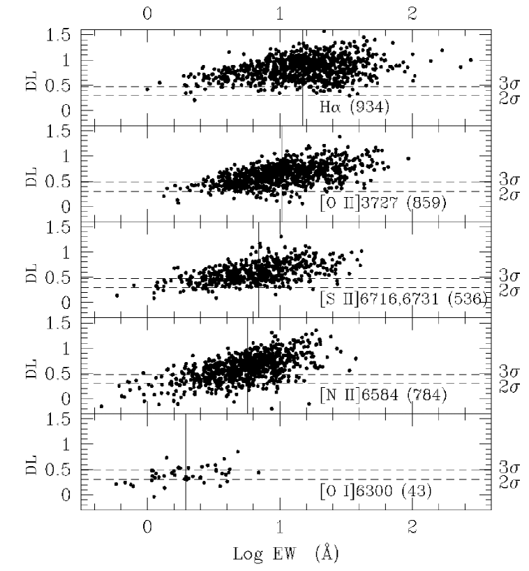
Figure 2. Top panel: Log of the detection level of EW(H$\alpha$), i.e. DL $=$ Log (EW/$\sigma$(EW)), versus Log EW(H$\alpha$). Lower panels: Same but for [O II] $\lambda$3727, for [S II] $\lambda\lambda$6716, 6731, for [N II] $\lambda$6584, and for [O I] $\lambda$6300. Vertical solid lines are the respective EW medians (see Table 3). The number of plotted data and the 2, $3\sigma$ detection levels (dashed lines) are indicated in each panel.

Figure 4. Top panel: Physical size at 25 mag arcsec^-2, $S_{25}$, as a function of the cosine inclination angle, cos($i$). Middle panel: Distributions of cos($i$), the shaded histogram is for unclassified galaxies (see Sect. 3.1). Bottom panel: Fractions of ELG as a function cos($i$), the mean is $61\%$ (dashed-dotted line).

Figure 6. Top panel: N($b_{J}$) distributions, the shaded histogram is for the $82$ unclassified galaxies (see Sect. 3.1). Bottom panel: Fraction of ELG as a function of $b_{J}$, the mean is $61\%$ (dashed-dotted line).

Figure 7. Top panel: N(z) distributions. Bottom panel: Fraction of ELG as a function of $z$. Notation the same as in Figure 6.

Figure 8. Top panel: N(M($b_{J}$)) distributions. Bottom panel: Fraction of ELG as a function of M($b_{J}$). Notation the same as in Figure 6.

Figure 9. Top panel: Physical size $S_{25}$ distributions. Bottom panel: Fraction of ELG as a function of $S_{25}$. Notation the same as in Figure 6.

Figure 10. Top panel: Rest-frame surface brightness $\mu_{25}$ distributions. Bottom panel: Fraction of ELG as a function of $\mu_{25}$. Notation the same as in Figure 6.

Figure 11. Top panel: D₄₀₀₀ distributions. Bottom panel: Fraction of ELG as a function of D₄₀₀₀ . Notation the same as in Figure 6.

Figure 12. M($b_{J}$) versus D₄₀₀₀

Figure 13. Top panel: N(M(B_AB)) distributions for the 138 CFRS galaxies at $z<0.3$, with H$\alpha$ detected (ELG) and with no H$\alpha$ detected (non-ELG). Bottom panel: Fraction of CFRS ELG as a function of M(B_AB).

Figure 14. Top panel: M($b_{J}$) distributions for the 934 ELG, for the 467 EW(H$\alpha$) $>$ 15 Å ELG (dashed line), and for the 467 EW(H$\alpha$) $\leq$ 15 Å (dotted line). Arrows are the respective medians (see Table 3). Bottom panel: Fraction of EW(H$\alpha$) $>$ 15 Å ELG as a function of M($b_{J}$).

Figure 15. Top panels: EW distributions of H$\alpha$, [O II] $\lambda$3727, [S II] $\lambda\lambda$6716, 6731, [N II] $\lambda$6583 and [O I] $\lambda$6300 for bright $M(b_{J})\leq-21$ (or $L\geq L^{*}_{B}$) ELG (dotted lines), and faint ($L<L^{*}_{B}$) ELG (dashed lines). Arrows are the respective medians (see Table 3). Bottom panels: Respective fractions of faint ELG as a function of EW.

Figure 16. Top panels: EW distributions of H$\alpha$, [O II] $\lambda$3727, [S II] $\lambda\lambda$6716, 6731 and [N II] $\lambda$6583 lines for high $D_{4000}\geq 1.4$ ELG (dotted lines), and low $D_{4000}<1.4$ ELG (dashed lines). Arrows are the respective medians (see Table 3). Bottom panels: Respective fractions of low D₄₀₀₀ ELG as a function of EW.

Figure 17. Distribution of the EW ratios for [N II] $\lambda$6583/H$\alpha$, [S II] $\lambda\lambda$6716,6731/H$\alpha$ and [O I] $\lambda$6300/H$\alpha$ (solid line). The dashed line is for 57 galaxies from K92’s sample weighted as described in Section 6.1.

Figure 19. Log EW([N II] $\lambda$6583) versus Log EW(H$\alpha$). Small symbols are data detected below $3\sigma$, large symbols are $>3\sigma$ data. AGN candidates ([N II] $\lambda$6563/H$\alpha>0.63$) are denoted by stars and non-AGN by filled circles. The solid line is the correlation using all ($>3\sigma$) data; EW([N II]) $\approx 0.4$ EW(H$\alpha$) (see Table 4). The average $1\sigma$ EW errorbars are also shown.

Figure 20. Log EW([S II] $\lambda\lambda$6716, 6731) versus Log EW(H$\alpha$). Same notation as Figure 19. EW([S II]) $\approx 0.4$ EW(H$\alpha$) (see Table 4).

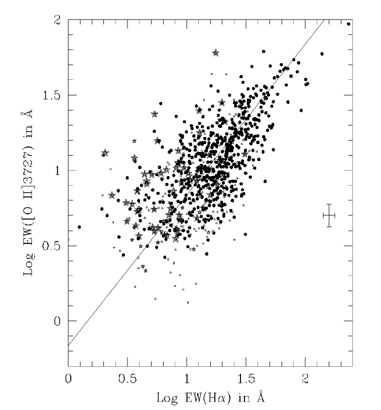
Figure 21. Log EW([O II] $\lambda$3727) versus Log EW(H$\alpha$). Same notation as Figure 19. EW([O II]) $\approx 0.7$ EW(H$\alpha$) (see Table 4).

Figure 23. Log EW([O I] $\lambda 6300$) versus Log EW(H$\alpha$). Same notation as Figure 19. EW([O I]) $\approx 0.1$ EW(H$\alpha$); note the correlation is very poor (see Table 4).

Figure 24. Log EW([O II] $\lambda$3727) versus Log EW(H$\alpha$ + [N II] $\lambda\lambda$6548, 6583). Dots are SAPM data, and the line shows the correlation from Figure 22. Filled symbols show K92 data (diamonds are AGN galaxies excluding Seyfert1) and open symbols show CFRS-12 data.

Figure 25. Relative distributions of EW([O II] $\lambda 3727$). (a) For the 1008 SAPM spectra with [O II] detected (solid line), and for the 68 spectra with [O II] but not H$\alpha$ detected (dotted line). The curve is reproduced from figure 9 in Kennicutt 1992, which shows the distribution of very nearby galaxies. (b) For the 1008 SAPM data (thick-solid line), for 55 CFRS-12 data at $0.2<z<0.3$ (thin-solid line), and for 403 CFRS-14 data ($0.2<z<1.3$; Hammer et al. 1997) (dashed line). Medians of the distributions are listed in Table 5.

Figure 1: Top panels: The complete rest-frame wavelength range spanned by one SAPM spectrum at $z=0.0534$. One can see the small gaps in continuum at (observed frame) $\sim$[4360–4370]Å, and $\sim$[7000–7020]Å (see Section 2.1). Bottom-left panel: Zoomed view of [O II] $\lambda$3727. Bottom-right panel: Zoomed view of [N II] $\lambda$6548, H$\alpha$, [N II] $\lambda$6583, [S II] $\lambda\lambda$6716, 6731 respectively.

Figure 2: Top panel: Log of the detection level of EW(H$\alpha$), i.e. DL $=$ Log (EW/$\sigma$(EW)), versus Log EW(H$\alpha$). Lower panels: Same but for [O II] $\lambda$3727, for [S II] $\lambda\lambda$6716, 6731, for [N II] $\lambda$6584, and for [O I] $\lambda$6300. Vertical solid lines are the respective EW medians. The number of plotted data and the 2, $3\sigma$ detection levels (dashed lines) are indicated in each panel.

Figure 3: For the whole sample (1671), fractions of the galaxy image covered by the 8″ wide slit if the slit was positioned along the major axis, $F(a)$, or the minor axis, $F(b)$, as a function of the physical size at 25 mag arcsec^-2, $S_{25}$ (upper panels), the cosine inclination angle, cos($i$) (middle panels), and the redshift, $z$ (lower panels).

Figure 4: Top panel: Physical size at 25 mag arcsec^-2, $S_{25}$, as a function of the cosine inclination angle, cos($i$). Middle panel: Distributions of cos($i$), the shaded histogram is for the 82 unclassified galaxies (see Sect. 3.1). Bottom panel: Fractions of ELG as a function cos($i$), the mean is $61\%$ (dashed-dotted line).

Figure 5: Log EW(H$\alpha$), and detection level of EW(H$\alpha$) as a function of the fraction of the galaxy image covered if the slit was positioned along the major axis, $F(a)$ (upper panels), the cosine inclination angle, cos($i$) (middle panels), and the redshift, $z$ (lower panels).

Figure 6: Top panel: N($b_{J}$) distributions, the shaded histogram is for the $82$ unclassified galaxies (see Sect. 3.1). Bottom panel: Fraction of ELG as a function of $b_{J}$, the mean is $61\%$ (dashed-dotted line).

Figure 7: Top panel: N(z) distributions. Bottom panel: Fraction of ELG as a function of $z$. Notation the same as in Figure 6.

Figure 8: Top panel: N(M($b_{J}$)) distributions. Bottom panel: Fraction of ELG as a function of M($b_{J}$). Notation the same as in Figure 6.

Figure 9: Top panel: Physical size $S_{25}$ distributions. Bottom panel: Fraction of ELG as a function of $S_{25}$. Notation the same as in Figure 6.

Figure 10: Top panel: Rest-frame surface brightness $\mu_{25}$ distributions. Bottom panel: Fraction of ELG as a function of $\mu_{25}$. Notation the same as in Figure 6.

Figure 11: Top panel: D₄₀₀₀ distributions. Bottom panel: Fraction of ELG as a function of D₄₀₀₀ . Notation the same as in Figure 6.

Figure 12: M($b_{J}$) versus D₄₀₀₀.

Figure 13: Top panel: N(M(B_AB)) distributions for the 138 CFRS galaxies at $z<0.3$, with H$\alpha$ detected (ELG) and with no H$\alpha$ detected (non-ELG). Bottom panel: Fraction of CFRS ELG as a function of M(B_AB).

Figure 14: Top panel: M($b_{J}$) distributions for the 934 ELG, for the 467 EW(H$\alpha$) $>$ 15 Å ELG (dashed line), and for the 467 EW(H$\alpha$) $\leq$ 15 Å (dotted line). Arrows are the respective medians (see Table 3). Bottom panel: Fraction of EW(H$\alpha$) $>$ 15 Å ELG as a function of M($b_{J}$).

Figure 15: Top panels: EW distributions of H$\alpha$, [O II] $\lambda$3727, [S II] $\lambda\lambda$6716, 6731, [N II] $\lambda$6583 and [O1] $\lambda$6300 for bright $M(b_{J})\leq-21$ (or $L\geq L^{*}_{B}$) ELG (dotted lines), and faint ($L<L^{*}_{B}$) ELG (dashed lines). Arrows are the respective medians (see Table 3). Bottom panels: Respective fractions of faint ELG as a function of EW.

Figure 16: Top panels: EW distributions of H$\alpha$, [O II] $\lambda$3727, [S II] $\lambda\lambda$6716, 6731, [N II] $\lambda$6583 and [O I] $\lambda 6300$ for high $D_{4000}\geq 1.4$ ELG (dotted lines), and low $D_{4000}<1.4$ ELG (dashed lines). Arrows are the respective medians (see Table 3). Bottom panels: Respective fractions of low D₄₀₀₀ ELG as a function of EW.

Figure 17: Distribution of the EW ratios for [N II] $\lambda$6583/H$\alpha$, [S II] $\lambda\lambda$6716,6731/H$\alpha$ and [O I] $\lambda$6300/H$\alpha$ (solid line). The dashed line is for 57 galaxies from K92’s sample weighted as described in Section 6.1.

Figure 18: (a) Log [N II] $\lambda$6583/H$\alpha$ versus Log EW(H$\alpha$). (b) Log 1.33 [N II] $\lambda$6583/H$\alpha$ versus Log EW(H$\alpha$ + 1.33[N II] $\lambda$6583). Dots are SAPM ($>3\sigma$) data, crosses are SAPM ($<3\sigma$) data. Open symbols are K92 high-resolution data, filled symbols are K92 low-resolution data. Triangles are AGN and circles are normal galaxies in K92 sample. The dotted line is the empirical separation between AGN and H ii galaxies. The solid line is the commonly used average value for [N II]/H$\alpha$. The diagonal line is our best fit to the correlation.

Figure 19: Log EW([N II] $\lambda$6583) versus Log EW(H$\alpha$). Small symbols are data detected below $3\sigma$, large symbols are $>3\sigma$ data. AGN candidates ([N II] $\lambda$6563/H$\alpha>0.63$) are denoted by stars and non-AGN by filled circles. The solid line is the correlation using all ($>3\sigma$) data; EW([N II]) $\approx 0.4$ EW(H$\alpha$) (see Table 4). The average $1\sigma$ EW errorbars are also shown.

Figure 20: Log EW([S II] $\lambda\lambda$6716, 6731) versus Log EW(H$\alpha$). Same notation as Figure 19. EW([S II]) $\approx 0.4$ EW(H$\alpha$) (see Table 4).

Figure 21: Log EW([O II $\lambda$3727]) versus Log EW(H$\alpha$). Same notation as Figure 19. EW([O II]) $\approx 0.7$ EW(H$\alpha$) (see Table 4).

Figure 22: Log EW([O II] $\lambda 3727$) versus Log EW(H$\alpha$ + [N II] $\lambda\lambda$6548, 6583). Same notation as Figure 19. EW([O II]) $\approx 0.5$ EW(H$\alpha$ + [N II]) (see Table 4).

Figure 23: Log EW([O I] $\lambda 6300$) versus Log EW(H$\alpha$). Same notation as Figure 19. EW([O I]) $\approx 0.1$ EW(H$\alpha$); note the correlation is very poor (see Table 4).

Figure 24: Log EW([O II] $\lambda 3727$) versus Log EW(H$\alpha$ + [N II] $\lambda\lambda$6548, 6583). Dots are SAPM data, and the line shows the correlation from Figure 22. Filled symbols show K92 data (diamonds are AGN galaxies excluding Seyfert1) and open symbols show CFRS-12 data.

Figure 25: Relative distributions of EW([O II] $\lambda 3727$). (a) For the 1008 SAPM spectra with [O II] detected (solid line), and for the 68 spectra with [O II] but not H$\alpha$ detected (dotted line). The curve is reproduced from figure 9 in Kennicutt 1992, which shows the distribution of very nearby galaxies. (b) For the 1008 SAPM data (thick-solid line), for 55 CFRS-12 data at $0.2<z<0.3$ (thin-solid line), and for 403 CFRS-14 data ($0.2<z<1.3$; Hammer et al. 1997) (dashed line). Medians of the distributions are listed in Table 5.

References

- [1998] Brinchmann J., Abraham R., Schade D., Tresse L. et al., 1998, ApJ, 499, 112
- [1983] Bruzual G., 1983, ApJ, 273, 105
- [1993] Bruzual G., Charlot S., 1993, ApJ, 405, 538
- [1990] Garnett D. R., 1989, ApJ, 363, 142
- [1998] Gallego J., Zamorano J., García–Dabò C. E., Aragón–Salamanca A., Guzmán R., 1998, in D’Odorico S., Fontana A., Giallongo E., eds, The Young Universe, A.S.P. Conference Series Vol. 146, p. 235
- [1997] Hammer F., Flores H., Lilly S., Crampton D., Le Fèvre O., Rola C., Mallen–Ornelas G., Schade D., Tresse L., 1997, ApJ, 481, 49
- [1997a] Ho L. C., Filippenko A. V., Sargent W. L., 1997a, ApJS, 112, 315
- [1997b] Ho L. C., Filippenko A. V., Sargent W. L., 1997b, ApJ, 487, 568
- [1997c] Ho L. C., Filippenko A. V., Sargent W. L., 1997c, ApJ, 487, 579
- [1983] Hodge P.W., Kennicutt, R. C., 1983, ApJ, 267, 563
- [1926] Hubble E., 1926, ApJ, 64, 321
- [1998] Hunter D. A., Elmegreen B. G., Baker A. L., 1998, ApJ, 493, 595
- [1999] Isotov Y. I, Thuan T. X., 1999, ApJ, 511, 639
- [1992] Kennicutt R. C., 1992, ApJ, 272, 54 (K92)
- [1983] Kennicutt R. C., Kent S. M., 1983, AJ, 88, 1094
- [1998] Kobulnicky H. A., Skillman E. D., 1998, ApJ, 497, 601
- [1996] Loveday J., 1996, MNRAS, 278, 1025
- [1999] Loveday J., Lilly, S. J., in preparation
- [1992] Loveday J., Peterson B. A., Efstathiou G., Maddox S. J., 1992, ApJ, 390, 338
- [1996] Loveday J., Peterson B. A., Maddox S. J., Efstathiou G., 1996, ApJS, 107, 201
- [1999] Loveday J., Tresse L., Maddox S. J., 1999, MNRAS, in press
- [1990] Maddox S. J., Sutherland W. J., Efstathiou G., Loveday J., 1990, MNRAS, 243, 692
- [1990b] Maddox S. J., Sutherland W. J., Efstathiou G., Loveday J., Peterson B. A. 1990, MNRAS, 247, 1p
- [1995] Maiolino R., Rieke G. H., 1995, ApJ, 454, 95
- [1989] Osterbrock D. E., 1989, Astrophysics of Gazeous Nebulae and Active Galactic Nuclei, Univ. Sci. Books
- [1994] Ryder S. D., Dopita M. A., 1994, ApJ, 430, 142
- [1981] Sandage A., Tammann G. A., 1981, A Revised Shapley–Ames Catalog of Bright Galaxies (Washington, DC: Carnegie Institution of Washington) (RSA)
- [1997] Schaerer D., de Koter A., 1997, A&A, 322, 598
- [1998] Tresse L., Maddox S. J., 1998, ApJ, 495, 691
- [1996] Tresse L., Rola C., Hammer F., Stasińska G., Le Fèvre O., Lilly S. J., Crampton D., 1996, MNRAS, 281, 847
- [1998] Tresse L., Maddox S. J., Loveday J., 1998, in D’Odorico S., Fontana A., Giallongo E., eds, The Young Universe, A.S.P. Conference Series Vol. 146, p. 330
- [1987] Veilleux S., Osterbrock D. E., 1987, ApJS, 63, 295
- [1986] Véron–Cetty M. P., Véron P., 1986, A&AS, 66, 335
- [1994] Zucca E., Pozetti L., Zamorani G., 1994, MNRAS, 269, 953