Supersonic Turbulence in the Perseus Molecular Cloud

Abstract

We compare the statistical properties of J=1$\rightarrow$0 ¹³CO spectra observed in the Perseus Molecular Cloud with synthetic J=1$\rightarrow$0 ¹³CO spectra, computed solving the non–LTE radiative transfer problem for a model cloud obtained as solutions of the three dimensional magneto–hydrodynamic (MHD) equations. The model cloud is a randomly forced super–Alfvénic and highly super–sonic turbulent isothermal flow.

The purpose of the present work is to test if idealized turbulent flows, without self–gravity, stellar radiation, stellar outflows, or any other effect of star formation, are inconsistent or not with statistical properties of star forming molecular clouds.

We present several statistical results that demonstrate remarkable similarity between real data and the synthetic cloud. Statistical properties of molecular clouds like Perseus are appropriately described by random supersonic and super–Alfvénic MHD flows. Although the description of gravity and stellar radiation are essential to understand the formation of single protostars and the effects of star formation in the cloud dynamics, the overall description of the cloud and of the initial conditions for star formation can apparently be provided on intermediate scales without accounting for gravity, stellar radiation, and a detailed modeling of stellar outflows

We also show that the relation between equivalent line width and integrated antenna temperature indicates the presence of a relatively strong magnetic field in the core B1, in agreement with Zeeman splitting measurements.

ppadoan@cfa.harvard.edu

1 Introduction

The structure and dynamics of molecular clouds (MCs) has been the subject of intensive investigation during the past two decades. Since MCs are the sites of star formation, their properties provide insights into the initial conditions needed to form stars. On the other hand, energy injected into the clouds by young stars is also believed to play a crucial role in the cloud dynamics and evolution (e.g. Whitworth 1979; Bally & Lada 1983; Miesch & Bally 1994). The observed state of a cloud represents the balance between energy injection and dissipation.

Observations show that cloud internal motions are highly supersonic, incoherent, and random (e.g. Bally et al. 1987, 1989, 1990). Furthermore, the cloud structure is complex and by many measures is suggestive of the presence of random flows. Indeed, many authors have attempted to describe clouds using various models of turbulence (e.g. Ferrini, Marchesoni & Vulpiani 1983; Henriksen & Turner 1984; Scalo 1987; Fleck 1988; Fleck 1996) inspired by the scaling laws observed in the interstellar medium (Larson 1981). More recently, there have been several attempts to describe cloud morphology and velocity fields using fractals (e.g. Scalo 1990; Falgarone & Phillips 1991; Falgarone, Phillips & Walker 1991; Falgarone 1992; Larson 1995; Elmegreen 1997).

Most theoreticians have argued that clouds are supported by magnetic fields (Mestel 1965; Strittmatter 1966; Parker 1973; Mouschovias 1976a, b; McKee & Zweibel 1995) and interpreted the observed line–widths in terms of magneto–hydrodynamic (MHD) waves (Arons & Max 1975; Zweibel & Josafatsson 1983; Elmegreen 1985, Falgarone & Puget 1986). However, comparison of the extinction statistics with recent models of supersonic and super–Alfvénic random flows suggests that such models may provide a superior description of MCs (Padoan, Jones & Nordlund 1997). Zeeman splitting measurements (for example Crutcher et al. 1993; Crutcher et al. 1996) have also been shown to be consistent with the predictions of a super–Alfvénic random flow (Padoan & Nordlund 1998).

In this paper, we compare some observed properties of the Perseus molecular cloud with the predictions of super–sonic and super–Alfvénic random flows. We start with a self–consistent MHD simulation of a random flow in a three dimensional $128^{3}$ grid. We solve the radiative transfer problem using a non–LTE Monte Carlo approach (Juvela 1997) to compute ¹³CO synthetic spectra on a 90 by 90 cell grid with 60 velocity channels. The experiment we use for the present paper is the same as model Ad1 in Padoan & Nordlund (1998), where a detailed description of the code is given. The method of obtaining synthetic spectra from our numerical simulations of MHD turbulence is presented in Padoan et al. (1998).

Super–sonic random flows can be shown to offer a natural interpretation of statistical and morphological properties of molecular clouds, at least for clouds that are not very active regions of star formation. For example, Padoan et al. (1998) calculate values of CO line intensity ratios and line width ratios, using synthetic spectra, that are very close to the values measured by Falgarone et al. (1991) and by Falgarone & Phillips (1996) in quiescent regions. It is normally believed that the study of molecular clouds that are actively forming stars requires instead a complicated modeling of the effect of star formation, such as energy injection from molecular outflows, HII regions, and so on. If this were true, it would be very difficult to learn general statistical properties of star forming molecular clouds, directly from numerical simulations of MHD flows. The present paper addresses this problem, by comparing statistical properties of super–sonic and super–Alfvénic turbulent flows with the same properties in the Perseus molecular cloud complex, which is a well known star formation site. The comparison between the model and the observations shows that a reasonable description of the kinematics and structure of molecular clouds can be provided by a turbulent flow model, that does not account for gravity, stellar radiation fields, stellar outflows, or any other effect of star formation.

2 The Perseus Molecular Cloud

Observations of the Perseus molecular cloud complex were made from 1985 to 1991 with AT&T Bell Laboratories 7 m offset Cassegrain antenna in Holmdel, New Jersey. Approximately a 6^∘ by 4^∘ region was surveyed in the 110 GHz line of J=1$\rightarrow$0 ¹³CO. The observations were made on a 1^′ grid with a 100^′′ beam yielding 33,000 spectra, each with 128 $\times$ 100 kHz channels (0.273 km s^-1). See Billawala et al. (1997) for further details of observations and discussion of the cloud structure.

The Perseus molecular cloud is roughly a 6^∘ by 2^∘ region located at a distance estimated to range from 200 to 350 pc (Herbig & Jones 1983; Cêrnis 1990) and has a projected size of 30 by 10 pc (see figure 1). The cloud is part of the larger Taurus–Auriga–Perseus complex and lies below the galactic plane (b $\sim\ -20^{\circ}$) with an estimated mass of 10⁴ M_⊙ (Billawala et al. 1997).

The complex has produced some high mass stars at its eastern end which lie near the centroid of the Perseus OB2 association, a loose grouping of 5 to 10 O and B stars, that is about 7 million years old (Blaauw 1991). Perseus OB2 has blown a 20^∘ diameter (100 pc) supershell into the surrounding interstellar medium that can be seen in 21 cm H ${\sc i}$ data (Heiles 1984). The shell is partially superimposed on the Perseus molecular cloud and may be interacting with it. Perseus contains two young stellar clusters and a background of relatively inactive molecular gas that has formed few stars.

Near the eastern end is the young ($<$ 7 Myr old) cluster IC348, which has several hundred members and may still be forming (Strom, Grasdalen & Strom 1974; Lada, Strom & Myers 1993; Lada & Lada 1995). Omicron Persei, a B1 III star, located near the center, is believed to be a few parsecs in front of the cloud (Bachiller et al. 1987). Lada & Lada (1995) estimate a cluster population of $\approx$ 380 stars with a highly centralized distribution falling off inversely with distance from the inner 0.1 pc diameter core which contains about $\sim$ 200 M_⊙ of stars and a density of 220 M_⊙ pc^-3. Star formation has been going on for at least 5 to 7 Myr at a roughly constant rate and with an efficiency of $\sim~{}50\%$.

A second and even younger cluster is embedded in the Perseus cloud several degrees to the west near the reflection nebula NGC1333. This region contains the most active site of ongoing star formation in Perseus. NGC1333 contains an embedded $<$ 1 Myr old infrared cluster, a large number of molecular outflows (Sandell & Knee 1998), Herbig–Haro objects (Bally, Devine & Reipurth 1996), and shock excited near–infrared H₂ emission regions (Aspin, Sandell & Russell 1994; Hodapp & Ladd 1995; Sandell et al. 1994). Lada, Alves & Lada (1996) find 143 young stars in a 432 square arc–minute region with most being members of two prominent sub–clusters. More than half of these stars display infrared excess emission, a signature of young stellar objects. Lada et al. estimate the age of the cluster to be less than $10^{6}$ years with a star formation rate of $4~{}\times~{}10^{-5}$ M_⊙ yr^-1.

Away from IC348 and NGC1333, the Perseus cloud contains about a dozen dense cloud cores with low levels of star formation activity including the dark cloud B5 (Langer 1989; Bally, Devine, & Alten 1996) at its eastern end, the cold core B1 for which a magnetic field has been measured by means of OH Zeeman (Goodman et al. 1989; Crutcher et al. 1993), and the dark clouds L1448 and L1455 on the west end (Bally et al. 1997).

The cloud exhibits a wealth of sub–structures such as cores, shells, and filaments and dynamical structures including stellar outflows and jets, and a large scale velocity gradient. While emission at the western end of the complex lies mostly near v_lsr = 4 km s^-1 (L1448), the eastern end of the complex has a velocity of v_lsr = 10.5 km s^-1(B5). This may be an indication that we are seeing several smaller clouds partially superimposed along the line of sight (Cêrnis 1990).

3 The Model

A synthetic molecular cloud map containing grids of 90 $\times$ 90 spectra of J=1$\rightarrow$0 ¹³CO  has been computed with a non–LTE Monte Carlo code (Juvela 1997), starting from density and velocity fields that provide realistic descriptions of the observed physical conditions in MCs. The density and velocity fields are obtained as solutions of the magneto–hydrodynamic (MHD) equations in a 128³ grid and in both super–Alfvénic and highly super–sonic regimes of a random isothermal flow. The numerical experiment is the same as model Ad1 in Padoan & Nordlund (1998), where details about the code and different experiments are given. The method of calculating synthetic spectra from numerical simulations of MHD turbulence is presented in Padoan et al. (1998).

The numerical MHD flow that is used in the present work (model Ad1 of Padoan & Nordlund 1998) has initial rms Mach number ${\cal M}=10.6$ and initial rms alfvénic Mach number ${\cal M}_{A}=10.6$, where ${\cal M}$ is the ratio of the rms velocity of the flow divided by the speed of sound, and ${\cal M}_{A}$ is the rms velocity of the flow divided by the Alfvén velocity. The flow is randomly driven, but the driving and the initial conditions are such that the rms velocity decreases for the first two dynamical times. The snapshot we use for the present work corresponds to a time equal to almost two initial dynamical times, where the Mach numbers are ${\cal M}=7.7$ and ${\cal M}_{A}=2.5$. The alfvénic Mach number has decreased also due to the amplification of the magnetic energy caused by the strong compressions and by the stretching of magnetic field lines, in the initial evolution of the flow. Molecular clouds have internal random motions of similar Mach number on the scale of about 3.7 pc (assuming a kinetic temperature of about 10 K), where the mean density is $<n>\approx 540$ cm^-3. These are therefore the values of the linear size and gas density that are used in the radiative transfer calculations. The corresponding mass of the model is 1.7$\times$10³ M_⊙ (using a mean molecular weight of $\mu$ =2.6 to correct for He).

The gas density spans the range of values 6.8 cm^-3–3.3$\times$10⁴ cm^-3, which produces column density values over a range of almost two orders of magnitude. Models similar to this have already been shown to reproduce observed statistical properties of molecular clouds (Padoan, Jones & Nordlund 1997; Padoan et al. 1998; Padoan & Nordlund 1998). Although a version of our MHD code can include self–gravity, and the Monte Carlo radiative transfer code can include the stellar radiation field, we have chosen not to include gravity or any effect of star formation. In fact, the purpose of the present work is to investigate if such a highly idealized description of the dynamics of molecular clouds is consistent or not with statistical properties of star forming molecular clouds. While it is clear that gravity is eventually important for the collapse of single protostars, and molecular outflows are important energy sources, it might be that the dynamics and statistical properties of star forming molecular clouds are described rather well by a randomly forced MHD super–sonic flow, without gravity and without a specific energy injection mimicking stellar outflows.

4 Results

In order to compare the observed spectra with the synthetic ones, it is necessary to eliminate the contribution of the noise to the value of the statistical quantities computed with the observed spectra. This is especially true for the value of the kurtosis of the velocity profiles, since it is the statistics of highest order among the ones we compute. The noise is treated in the following way. First, the noise is estimated using velocity channels where no emission is apparently detected. The average antenna temperature in such velocity channels is -0.0009 K, and the rms value is 0.1556 K. Then the antenna temperature is set equal to zero in all velocity channels where it is lower than the $2\sigma$ value of the noise, that is 0.3 K. Finally, to avoid unphysical sharp features in the velocity profiles, due to the antenna temperature clipping, the spectra are smoothed, only in velocity channels with antenna temperature lower than 0.8 K, with a gaussian filter with a width of 5 velocity channels. We have verified that the final smoothing affects the statistical distributions very little, while the antenna temperature clipping is necessary to obtain any agreement between observational data and synthetic spectra. Although the choice of the clipping at the $2\sigma$ noise level is somewhat arbitrary, we point out that this choice not only allows an excellent fit of the distribution of kurtosis, but also allow a match, at the same time, of all other statistical distributions we have computed. A different clipping level, eliminates the good fit of all statistics at the same time. It remains to be checked if the same clipping level is valid for observed spectra with any value of signal to noise, or if spectra of different quality need to be treated with a different clipping level.

The synthetic integrated antenna temperature maps, computed from the model clouds solving the radiative transfer problem along the x, y and z axis, look rather filamentary (left panel of Fig. 2). The Perseus map (Fig. 1), instead, does not show a very filamentary morphology. However, the resolution of the observations is inferior to the resolution of the synthetic maps. To allow for a comparison, it is necessary to degrade the resolution of the synthetic map to a level comparable to the resolution in the observations. This has been done by filtering the maps with a gaussian filter with width approximately equal to twice the nominal size of the 100” observational beam. The morphology of the synthetic maps after filtering is not very different from the observed morphology; the underlying filamentation is hardly visible. In the same way, an intrinsic filamentation in the Perseus molecular cloud complex would be largely hidden from view in the present data, for lack of resolution.

Examples of grids of spectra are shown in Fig. 3 and Fig. 4. The original synthetic maps contain 90$\times$90 spectra, but only a subset of 30$\times$30 spectra is plotted here. Model and real clouds both show some spectra that are close to gaussian, and some other with multiple components. These spectra can be used to compute several statistical properties of the clouds. In Fig.s 5-8, different statistics are shown for regions around L1448, NGC1333, and B1. In each figure the histograms computed with the synthetic spectra are also overplotted for comparison (thick lines), and a small contour map of the selected region is shown. Since the model is not computed with the purpose of fitting any specific cloud, the histogram of velocity centroids, $<v>$, is not expected to match the observations. Such histograms depend in fact on the specific large scale motions inside each cloud.

The distribution of the standard deviation of single spectra, $\sigma(v)$, (the dispersion of radial velocity in each line of sight), can also be a tricky quantity to fit with a theoretical model. It may happen that two or more physically disconnected clouds are superposed on the line of sight and produce a spectrum with multiple components, at different velocities, which may cause a significant growth of the standard deviation. Multiple components are found also in the synthetic spectra, but are due to the superposition of structures that belong to the same cloud. The enhancement of $\sigma(v)$ can be important when large regions are sampled, because the chance of random superposition of disconnected clouds is large.

All other histograms plotted in Fig.s 5-8 do instead measure to what extent the model is consistent with the observations. Such statistics are the probability distribution of skewness and kurtosis of the spectra, that constrains the shape of the spectra; the probability distribution of equivalent line width, $\Delta v$; the probability distribution of velocity integrated antenna temperature, $\int Tdv$ (roughly proportional to column density); the relation between equivalent line width and integrated temperature. The distributions are computed by measuring all the above quantities in each line of sight.

4.1 L1448

A region around the cloud core L1448 has been selected, that contains also a part of the core L1455 (visible in the bottom left corner on the contour map in Fig. 5). The dark core L1448 contains a number of young stars and Herbig–Haro objects, but it is a relatively quiescent region in the cloud complex. Fig. 5 shows that the statistics of the theoretical model match almost exactly the statistics of the spectra of L1448.

In Fig. 6, the same statistical properties are plotted against each other, and again the agreement between the model and the observations is excellent. For example, both observed and synthetic spectra with large kurtosis (larger than gaussian) tend to have extreme values of skewness (negative or positive). Only the relations between kurtosis and line width seem to be significantly different between theory and observations. Similar results are obtained for other regions in the Perseus complex, and the equivalent of Fig. 6 for other regions is not shown in the following.

Figures 5 and 6 show that statistical properties of spectra observed around the core L1448 are well reproduced by the present idealized model, and therefore are likely to be related to super–sonic and super–Alfvénic turbulence present in the molecular gas.

4.2 NGC1333

The region around the reflection nebula NGC1333 is instead the most active site of ongoing star formation in the Perseus cloud complex. Molecular outflows, Herbig–Haro objects, and shock excited H₂ emission regions have been observed. The comparison of the model with NGC1333, in Fig. 7, shows that NGC1333 has slightly larger line width than the model. This is not surprising, since the model is not tailored to any particular cloud core. Consistently with the larger line width, the distribution of integrated temperature is also a bit broader than in the model. In fact, it is a feature of our models that flows with larger velocity dispersion (hence larger $\Delta v$) produce broader distributions of integrated temperature (Padoan et al. 1998), than flows with smaller velocity dispersion. The histograms of skewness and kurtosis match rather well the model, and the relation between equivalent line width and integrated antenna temperature is virtually identical to the theoretical one.

Even the very active region around NGC1333 has therefore statistical properties that are well described by the present idealized model of the dynamics of molecular clouds.

4.3 B1

The core B1 is very interesting because a rather strong magnetic field strength has been detected there (Goodman et al. 1989; Crutcher et al. 1993). The match between model and observations is again very good (Fig. 8), apart from the distribution of integrated antenna temperature and for the relation between line width and integrated temperature. The distribution of integrated temperature is perhaps affected by the very small size of the region selected around the core, that does not include a significant area of very low column density. Even in the synthetic maps one can select a small region around a core or a filament and obtain a distribution of integrated temperature similar to the one observed in the core B1.

The line width in B1 does not grow with integrated temperature, above the value of 2 K km/s, and even decreases slightly up to the value of 8 K km/s. This behavior of the line width is observed in our models with relatively strong magnetic field (rough equipartition of kinetic and magnetic energy), as shown in Padoan & Nordlund (1998). In the same work it is also shown that the formation of some cores with relatively strong magnetic field is also predicted in the context of a super–Alfvénic model for the cloud dynamics, such as the present model. The relation between equivalent line width and integrated antenna temperature in the core B1 is therefore in agreement with the strong field detected in this core with Zeeman splitting measurements, and is consistent with our super–sonic and super–Alfvénic turbulence model for the dynamics of molecular clouds.

5 Discussion and Results

5.1 Observational and Synthetic Molecular Line Spectra

Several authors have developed theoretical models of dark clouds to interpret molecular line observations. Although the earliest interpretation of the carbon monoxide line profiles was that molecular clouds are collapsing (Goldreich & Kwan 1974; Liszt et al. 1974), it was soon realized that systematic motions different than collapse, or random motions were more likely explanations for the line profiles (Zuckerman & Evans 1974; Leung & Liszt 1976; Baker 1976; Kwan 1978; Albrecht & Kegel 1987). Models have then been improved with the use of clumpy density distributions, where the volume filling fraction of the clumps and their internal density are the main parameters (Kwan & Sanders 1986; Tauber & Goldsmith 1990; Tauber, Goldsmith & Dickman 1991; Wolfire, Hollenbach & Tielens 1993; Robert & Pagani 1993; Park & Hong 1995; Park, Hong & Minh 1996) and with the use of fractal density distributions (Juvela 1997).

Although velocity and density distributions used in such models are not related in any way to solutions of the fluid–dynamic equations, it was generally believed that some kind of MHD waves or hydro–dynamic turbulence should be at the origin of the random motions. Some studies have attempted to relate molecular cloud motions, as probed by line profiles, to turbulence. Falgarone & Phillips (1990) studied molecular line profiles of different sources, and found excess emission in the line wings, relative to a Gaussian distribution (see also Blitz, Magnani & Wandel 1988). Miesch & Bally (1994) computed autocorrelation and structure functions of line centroid velocities in five nearby mlecular clouds, and compare their results with phenomenological theories of turbulence. Miesch & Scalo (1995) looked at the histograms of emission line centroids, and found nearly exponential tails in many cases. Lis et al. (1996) studied the statistics of line centroids and of centroid increments, and found non-Gaussian behavior especially in the histograms of the velocity centroid increments.

Stenholm & Pudritz (1993) and Falgarone et al. (1994) calculated synthetic molecular spectra from fluid models of clouds. Stenholm & Pudritz (1993) used a sticky particles code with an imposed spectrum of Alfvén waves (Carlberg & Pudritz 1990). They calculated line profiles under the LTE assumption. Falgarone et al. (1994) did not solve the radiative transfer problem but calculated density weighted radial velocity profiles, using velocity and density fields from a numerical simulation of compressible turbulence by Porter, Pouquet & Woodward (1994). Padoan et al. (1998) calculated several maps of 90 by 90 synthetic spectra of different transitions of various molecules, using models and methods similar to the ones used here. Both the numerical models and the radiative transfer calculations constitute a significant improvement on the Falgarone et al. (1994) investigation. The numerical model used in that work (Porter et al. 1994) had Mach numbers close to unity, and therefore a relatively small density contrast, inconsistent with the density structure of molecular clouds, and in contradiction with the many models of line profiles that have proved the importance of the clumpy structure of molecular clouds (see references above). Moreover, while in Falgarone et al. (1994) the line profiles are calculated simply as density weighted radial velocity profiles, in Padoan et al. (1994) the line profiles are calculated by solving the radiative transfer problem, and line intensity ratios and line width ratios of different molecules or of different transitions of the same molecules are calculated, and shown to compare well with the observations.

According to Falgarone et al. (1994) the non–Gaussian shape of the line profiles in molecular clouds is the results of intermittency, and shocks make a minor contribution to the structure of the velocity field. Although this might be true for the simulations by Porter, Pouquet & Woodward (1994), that are transonic and so are characterized more by vortex tubes than by shocks, it cannot be true in the case of the highly super–sonic motions in molecular clouds. In the simulations of highly super–sonic turbulence by Padoan et al. (1998), the flows are characterized by a complex system of interacting shocks, that are responsible for the generation of large density contrasts, as observed in molecular clouds. Several of these velocity discontinuities are present along each line of sight through the cloud model, and must be an essential ingredient in the integrated velocity profile. The correlation between density and velocity fields is also essential, and can be studied appropriately only with highly super–sonic flows. The statement that intermittency is at the origin of the non–Gaussian shapes has been critisized in Dubinski, Narayan & Phillips (1995), where it is shown that non–Gaussian shapes arise trivially from steep power spectra, as the Kolmogorov power spectrum, similar to the one obtained in the simulation by Porter, Pouquet & Woodward (1994). Finally, Falgarone et al. (1994) do not discuss the role played by the magnetic field in the velocity profiles, since the magnetic field is not included in the calculations by Porter, Pouquet & Woodward (1994).

The present work follows the same method as in Padoan et al. (1998), but uses new runs with larger rms Mach number (up to 28), presented in Padoan & Nordlund (1998). The rms Mach number of the model used in this work, ${\cal M}=7.7$, is typical of motions inside molecular clouds, and therefore there is no need to rescale the density field in order to mimick a larger Mach number, as in Padoan et al. (1998). It has been shown that the distributions of skewness and curtosis of the synthetic line profiles of single line of sight matches very well the same distributions for the line profiles observed in molecular clouds of the Perseus complex. The match is very good also between theoretical and observed integrated temperature distributions, and integrated temperature versus equivalent width relations. The Perseus complex has been chosen because it is a well known site of ongoing star formation, and it is an important question wether the effect of star formation activity change drastically the statistical properties of molecular cloud motions, or if such motions can still be described statistically with idealized models of turbulent flows, without self gravity, radiation field, and stellar outflows.

Padoan & Nordlund (1998) proposed to use the relation between the integrated temperature and the equivalent width to estimate the dynamic importance of the magnetic field in molecular clouds, following an earlier suggestion by Heyer, Carpenter & Ladd (1996). This relation is normally found to be consistent with the motions being super–Alfvénic (Heyer, Carpenter & Ladd 1996; Padoan & Nordlund 1998). We have verified this also in the case of the Perseus complex: the equivalent line width always grows with increasing integrated antenna temperature. Only in the case of the core B1 have we found that the line width does not grow, or even decreases, with increasing integrated antenna temperature. According to our models, this indicates the presence of a strong magnetic field, with a rough equipartition of magnetic and kinetic energy. The core B1 is in fact the single spot in the Perseus complex where a relatively strong magnetic field has been succesfully detected (Goodman et al. 1989; Crutcher et al. 1993), and is believed to be important in the dynamics of the core. This example illustrates that the inclusion of the magnetic field in a cloud model can be important to the interpretation of the line profiles, and gives further support to the idea that the dynamics of molecular clouds is essentially super–Alfvénic (Padoan & Nordlund 1998), because if that was not the case, the line width versus integrated temperature relation would always look like the one in the core B1, contrary to the observational evidence, and because the formation of cores with strong magnetic field is predicted in the super–Alfvénic model (Padoan & Nordlund 1998).

5.2 Super–Sonic Turbulence in Molecular Clouds

The model used in this work is consistent with general observed properties of dark clouds such as the existence of random and supersonic motions, but it is not tailored to the specific characteristics of the Perseus molecular cloud or individual cores. Only the general interstellar medium scaling laws (Larson 1981) have been used to fix the physical size of the cloud model, and the comparison of the model with the observational data is justified by their similar size, inner scale (resolution) and line widths.

The dynamic range of length scales covered by the MHD calculations extends from 0.03 pc to 3.7 pc (128³ grid–points). The radiative transfer calculations and the resulting spectra cover a linear scale range from 0.04 pc to 3.7 pc (90³ grid–points). However, numerical dissipation effectively degrades this resolution by a factor of two to an inner scale of about 0.06 pc. Thus the inner scale of the theoretical models is about half of the linear resolution of the 100^′′ beam used in our observations. The Bell Labs 7 meter telescope beam has a linear resolution of about 0.14 pc (assuming a distance of 300 pc for the Perseus cloud) and the maximum extent of the Perseus cloud that has been mapped is about 30 pc. If the Perseus cloud is interpreted as an elongated single cloud, its typical thickness is about 4 pc; if it is interpreted as a line–of–sight superposition of different clouds, then each cloud has a size of about 4 pc. These sizes are also comparable to the linear size of the numerical model. Moreover, average spectra from single components of the Perseus cloud, and line widths of single line–of–sights are also comparable to the ones in the model.

Giant molecular clouds (GMCs; M$~{}>~{}10^{5}$ M_⊙ and L $\approx$ 20 to 50 pc) are gravitationally bound. This must be the case since the product of the internal velocity dispersion squared times the density is one to two orders of magnitude greater than the pressure of the surrounding interstellar medium. Gravity must provide the restoring force on the scale of a GMC, otherwise GMCs would be dispersed before they could form any stars. Individual stars form from the gravitational contraction of small cores with sizes of order 0.1 pc, while clusters of stars such as IC348 and NGC1333 form from cores about 1 pc in diameter. Thus gravity is certainly important on the very large scale of GMCs (L $>$ 20 pc) and on the very small scales of dense star forming cores (L $\leq$ 1 pc). Our model and observations have linear dimensions intermediate between these two scales. The results of this work show that on intermediate scales the observed properties of molecular clouds and likely the initial conditions for star formation can be appropriately described without explicitly accounting for gravity. Self–gravitating cores may occasionally condense from the random flow where a local over-density is produced statistically. However, at any one time, only a fraction of the total mass is involved in such condensations. If indeed self–gravitating cores condense out of a complex density field generated by super–sonic turbulent flows, then it might be possible to predict the mass spectrum of the resulting condensations which produce stars. This may be an important ingredient in constructing the initial stellar mass function (Padoan, Nordlund & Jones 1997).

In this picture, the overall density structure inside a GMC is not the result of gravitational fragmentation, but rather of the presence of supersonic random motions together with the short cooling time of the molecular gas. We predict that there are several shocks in the gas along any line–of–sight with velocities comparable to the overall cloud line–width. These shocks have velocities of order 1 to 10 km s^-1 which are not observable in the forbidden lines in the visible portion of the spectrum. However, there are several far–infrared transitions such as the 157 $\mu$m fine–structure line of C⁺, the 63 $\mu$m line of O i , and the 28, 17, and 12 $\mu$m v = 0–0 lines of H₂ which are readily excited by such shocks. The COBE and ISO satellites have shown that these transitions together carry about 0.1% of the total luminosity of a typical galaxy (Wright et al. 1991; cf. Lord et al. 1996). We predict that roughly 10% of this emission is produced by the shocks discussed above because these transitions are the important coolants in the post–shock gas.

The dissipation of the kinetic energy of internal motions, $E_{GMC}$, by shocks in a GMC produces a luminosity of order $L_{GMC}~{}\approx~{}E_{GMC}/\tau_{GMC}~{}\approx$ $3\times 10^{3}$ (L_⊙ ) $E_{51}\tau_{4\times 10^{6}}$ , where the dynamical time is taken to be a cloud crossing time, $\tau_{GMC}$ = $R_{GMC}/\sigma_{GMC}$ and $\sigma_{GMC}$ is the cloud velocity dispersion. Since the above infrared transitions are important coolants in the post–shock layers of these low velocity shocks, we expect that future observations of clouds like Perseus will show extended bright emission in these infrared transitions.

Observations of young stellar populations show that stars form from GMCs over a period of the order of 10 to 20 Myrs (Blaauw 1991) which implies that clouds must survive for at least this long. Since this time–scale exceeds the dissipation time, the internal motions must be regenerated. There are several possible sources for such energy generation. When massive stars are present, their radiation, winds, and supernova explosions inject large amounts of energy into the surrounding gas. However this amount of energy is far in excess of what is required to balance the dissipation of kinetic energy in shocks. Massive stars are likely to be responsible for cloud disruption.

The second candidate energy source is outflows from low mass stars which form more uniformly throughout the cloud (Strom et al. 1989; Strom, Margulis & Strom 1989). The Perseus molecular cloud contains only intermediate to low mass stars, which during their first $10^{5}$ years of life produced jets and outflows. All the cores studied here are known to have multiple outflows. Over a dozen outflows in NGC1333, 8 groups of Herbig–Haro objects in L1448, and 2 outflows in B5 have been discovered. Outflows can provide the mechanism to stir the clouds and balance the dissipation of the random supersonic motions.

However, the main source of energy for the small and intermediate scale differential velocity field may simply be cascading of energy from larger scales, where supernova activity is a likely source of galactic turbulence ([Korpi et al., 1998b, Korpi et al., 1998a, Korpi et al., 1999]). The dynamical times of inertial scale motions are short compared to those of the larger scale motions. In the inertial range, there is a quasi-stead flow of energy from larger scales towards the energy dissipation scales. The numerical simulations represents only piece of the inertial range, and hence, on these scales, energy input at the largest wavenumbers is to be expected.

6 Conclusions

Padoan, Jones & Nordlund (1997) and Padoan & Nordlund (1998) have shown that statistics of infrared stellar extinction (Lada et al. 1994) and OH Zeeman measurements (for example Crutcher et al. 1993; Crutcher et al. 1996) are consistent with the properties of supersonic random flows. Padoan et al. (1998) have calculated values of CO line intensity ratios and line width ratios, using synthetic spectra, that are very close to the values measured by Falgarone et al. (1991) and by Falgarone & Phillips (1996) in quiescent regions. In the present work, we have shown that idealized turbulent flows, without self–gravity, stellar radiation, stellar outflows, or any other effect of star formation, can also provide a description of statistical properties of molecular clouds that are actively forming stars. We have also shown, using the relation between integrated antenna temperature and equivalent line width, that the motions in the Perseus complex must be super–Alfvénic, with the exception of the core B1, where in fact a strong magnetic field has been detected. This is a further confirmation of the super-Alfvénic molecular cloud model proposed by Padoan & Nordlund (1998), where the formation of cores with relatively strong magnetic field is also predicted.

It can be concluded therefore that super–sonic and super–Alfvénic randomly forced turbulence correctly describes the structure and dynamics of molecular clouds, even when they are apparently affected by star formation. This cannot be truly surprising, because, no matter what the energy sources are, the motions in molecular clouds must be highly turbulent, due to the very large Reynolds number, and statistical properties of turbulence such as probability density functions are universal, both in nature and in computer simulations.

Figure captions:

Figure 1: Integrated antenna temperature of J=1$\rightarrow$0 ¹³CO for velocities 0 to 15 km s^-1 

Figure 2: Integrated antenna temperature of the model cloud (left and middle panels) and of L1448 (right panel). The middle and the right panels have been smoothed with a gaussian filter of width comparable with the 100” observational beam. The left panel is also smoothed with a gaussian filter, but the width is comparable with the grid size.

Figure 3: A 30 $\times$ 30 map of individual J=1$\rightarrow$0 ¹³CO synthetic spectra from the model cloud. The velocity interval in the plots is 6.0 km s^-1 and the antenna temperature ranges from 0 to 6 K. The original map contains 90 $\times$ 90 synthetic spectra.

Figure 4: A 30 $\times$ 30 map of individual J=1$\rightarrow$0 ¹³CO observed spectra of L1448. The velocity interval in the plots is 6.3 km s^-1 and the antenna temperature ranges from 0 to 6 K.

Figure 5: The top four panels: Distribution of centroid velocities (upper left); distribution of line widths (upper right); distribution of skewness (lower left); and distribution of kurtosis (lower right). The bottom four panels: Contour map of integrated temperature of the selected region (upper left); distribution of equivalent width (upper right); distribution of integrated antenna temperature (lower left); and equivalent width versus integrated antenna temperature (lower right). Thick lines are computed using spectra of single lines of sight from the model cloud. Thin lines are from the region around the core L1448.

Figure 6: Correlations between different properties of the theoretical spectra (thick lines) and of the spectra of the region around the core L1448 (thin lines).

Figure 7: Same as Fig. 5, but for the region around the core NGC1333.

Figure 8: Same as Fig. 5, but for the region around the core B1.

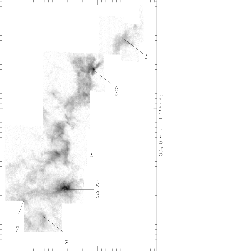
Figure 1:

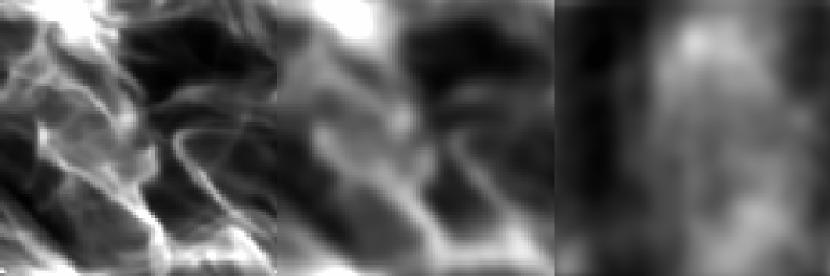
Figure 2:

Figure 3:

Figure 4:

Figure 5:

Figure 6:

Figure 7:

Figure 8: