OUTER REGIONS OF THE CLUSTER GASEOUS ATMOSPHERES

Abstract

We present a systematic study of the hot gas distribution in the outer regions of regular clusters using ROSAT PSPC data. Outside the cooling flow region, the $\beta$-model describes the observed surface brightness closely, but not precisely. Between 0.3 and 1 virial radii, the profiles are characterized by a power law with slope, expressed in terms of the $\beta$ parameter, in the range $\beta=0.65$ to $0.85$. The values of $\beta$ in this range of radii are typically larger by $\approx 0.05$ than those derived from the global fit. There is a mild trend for the slope to increase with temperature, from $\langle\beta\rangle\approx 0.68$ for 3 keV clusters to $\approx 0.8$ for 10 keV clusters; however, even at high temperatures there are clusters with flat gas profiles, $\beta<0.7$. Our values of $\beta$ at large radius are systematically higher, and the trend of $\beta$ with temperature is weaker than was previously found; the most likely explanation is that earlier studies were affected by an incomplete exclusion of the central cooling flow regions. For our regular clusters, the gas distribution at large radii is quite close to spherically symmetric and this is shown not to be an artifact of the sample selection. The gas density profiles are very similar when compared in the units of cluster virial radius. The radius of fixed mean gas overdensity 1000 (corresponding to the dark matter overdensity 200 for $\Omega=0.2$) shows a tight correlation with temperature, $R\sim T^{0.5}$, as expected from the virial theorem for clusters with the universal gas fraction. At a given temperature, the rms scatter of the gas overdensity radius is only $\approx 7\%$ which translates into a 20% scatter of the gas mass fraction, including statistical scatter due to measurement uncertainties.

Table 1Cluster Sample

Name	$z$	$T$	Ref.	$r_{\rm 180}(T)$	$R_{\rm cool}$	$N_{H}$	Note
		(keV)		(arcmin)	(arcmin)	($10^{20}\,$cm-2)
Cooling flow clusters
2A0335	$0.035$	$3.0\pm 0.1$	1	37.3	3.8a	18.12DD
A85	$0.052$	$6.9\pm 0.2$	2	39.0	1.8a	3.36DD	?
A133	$0.060$	$3.8\pm 0.8$	3	25.3	1.6b	1.58DD
A478	$0.088$	$8.4\pm 0.7$	2	27.0	1.5a	15.08DD
A496	$0.033$	$4.9\pm 0.1$	4	50.5	2.0a	4.79DD
A644	$0.071$	$8.1\pm 0.5$	2	32.0	1.3a	6.52DD
A780	$0.057$	$4.3\pm 0.2$	2	28.4	1.8a	4.84DD
A1651	$0.085$	$6.3\pm 0.3$	2	24.2	1.0a	1.88DD
A1689	$0.184$	$9.0\pm 0.2$	5	15.5	0.8a	1.81DD
A1795	$0.062$	$7.8\pm 0.6$	2	35.3	1.8a	1.17DD
A2029	$0.077$	$9.1\pm 0.6$	2	31.7	1.6a	3.15DD
A2052	$0.035$	$3.1\pm 0.2$	3	37.5	2.5a	2.84DD
A2063	$0.035$	$4.1\pm 0.6$	3	42.9	1.6a	3.04DD
A2142	$0.089$	$9.7\pm 0.8$	2	28.6	1.1a	4.16DD	?
A2199	$0.030$	$4.8\pm 0.1$	4	54.3	2.9a	0.89DD
A2597	$0.085$	$4.4\pm 0.3$	2	20.1	1.2a	2.49DD
A2657	$0.040$	$3.7\pm 0.2$	2	36.4	1.6b	5.57DD
A2717	$0.050$	$2.2\pm 0.5$	6	22.9	1.9c	1.11DD
A3112	$0.076$	$5.3\pm 0.5$	2	26.2	1.8a	2.53DD
A3571	$0.040$	$6.9\pm 0.1$	2	49.7	1.6a	4.11DD
A4038	$0.028$	$3.3\pm 0.8$	3	47.7	2.8a	1.54DD
A4059	$0.048$	$4.4\pm 0.2$	2	33.5	2.0a	1.10DD
AWM4	$0.032$	$2.4\pm 0.1$	1	36.0	1.0b	4.99DD
MKW3S	$0.045$	$3.7\pm 0.1$	2	32.6	2.4a	3.05DD
MKW4	$0.020$	$1.7\pm 0.1$	1	47.9	2.1b	1.88DD	?
Non-cooling flow clusters
A21	$0.095$	$5.3\pm 1.0$	7	20.1	…	4.44DD
A400	$0.024$	$2.3\pm 0.1$	1	46.8	…	9.39DD	?
A401	$0.074$	$8.0\pm 0.2$	2	30.6	0.7a	10.16DD
A539	$0.029$	$3.2\pm 0.1$	1	46.4	0.7b	12.77DD
A1413	$0.143$	$6.7\pm 0.2$	5	16.2	…	1.92DD
A2163	$0.203$	$13.9\pm 0.6$	3	18.0	…	12.01DD	?
A2218	$0.171$	$7.5\pm 0.3$	5	15.0	0.4b	3.14DD
A2255	$0.080$	$7.3\pm 1.0$	3	27.3	…	2.53DD
A2256	$0.058$	$7.3\pm 0.3$	2	36.4	…	4.07DD	?
A2382	$0.065$	$2.9\pm 0.7$	7	20.7	…	4.16DD
A2462	$0.075$	$2.5\pm 0.6$	6	16.9	…	3.07DD
A3301	$0.054$	$3.0\pm 0.7$	6	24.9	…	2.34DD
A3391	$0.054$	$5.4\pm 0.4$	2	33.4	…	5.48DD
Tri Aus	$0.051$	$9.6\pm 0.4$	2	46.9	0.9a	13.28DD

^a — Peres et al. (1998),  ^b — White et al. 1997,  ^c — our own estimate.

Temperature references: 1 — Fukuzawa et al. (1998), 2 — Markevitch et al. 1998, 3 — David et al. (1993), 4 — Markevtch et al. (1999), 5 — Mushotzky & Scharf (1997), 6 — our estimate from the $L-T$ correlation, 7 — Ebeling et al. (1996).

Question mark in the last column denotes those clusters with some substructure in the ROSAT image.

1. Introduction

Clusters of galaxies are very important tools for observational cosmology. Massive clusters form through collapse of a large volume and therefore thought to contain a fair sample of the Universe in terms of dark matter, diffuse baryons, and possibly stellar mass. Through the study of the relative contribution of these components in clusters, one can determine the average matter density in the Universe as a whole (White et al. 1993, Carlberg et al. 1996).

Most of mass in clusters is in the form of dark matter, observable directly only through the gravitational distortion of background galaxy images. For various reasons (sparseness, limited area coverage) lensing observations still cannot be used for a detailed study of the dark matter distribution in clusters. Much progress in understanding the dark matter halos of clusters has been done theoretically, through cosmological numerical simulations. Properties of simulated clusters in many respects agree with analytic or semi-analytic theoretical predictions. The mass function of clusters is in good agreement with that predicted by Press & Schechter (1974) theory (Efstathiou et al. 1985, Lacey & Cole 1994). A virialized region is well defined by $r_{180}$, a radius within which the mean density is approximately 180 of the critical density (Cole & Lacey 1996). Simulations predict that the dark matter density profiles are very similar when the radii are scaled to $r_{180}$, the hot gas follows the dark matter distribution at large radii, and these two components have equal temperature (Navarro, Frenk, & White 1995). As expected from the virial theorem, the gas temperature in simulations scales as $M_{180}\propto T^{3/2}$, where $M_{180}$ is the mass within $r_{180}$ (Evrard, Metzler, & Navarro 1996).

Most baryons, i.e. observable matter, in clusters are in the form of hot, X-ray emitting gas. Therefore, most of our direct knowledge about the structure of clusters comes from X-ray observations. Important cosmological conclusions derived from X-ray observations of clusters usually rely on simple theoretical assumptions. For example, a measurement of $\Omega$ from the baryon fraction in clusters (White et al. 1993, David, Jones, & Forman 1995, Evrard 1997) requires that cluster baryons are not segregated with respect to the dark matter. Measurement of the cosmological parameters from the evolution of the cluster temperature function (Henry 1997) relies on the converting of temperature to mass as $M\propto T^{3/2}$. However, unlike dark matter in simulated clusters, properties of the hot gas inferred from X-ray observations often deviate from simple theoretical expectations. For example, if gas were to follow the dark matter of Navarro et al. (1995), one would observe $\rho_{\rm g}\sim r^{-2.7}$ in the outer cluster parts (at $r\sim 1\,$Mpc), whereas the gas density profiles inferred from the Einstein observatory images are significantly flatter, $\rho_{\rm g}\sim r^{-1.8}$ (Jones & Forman 1984, 1998). The universal density profile, virial theorem, and the non-segregation of baryons predict the relation between X-ray luminosity and gas temperature $L\propto T^{2}$. The observed relation is significantly steeper, $L\sim T^{2.6-3}$ (David et al. 1993, Markevitch 1998, Allen & Fabian 1998). Using the gas temperature profile measured by ASCA and assuming that gas is in hydrostatic equilibrium, Markevitch & Vikhlinin (1997) derived the mass of A2256 which was found to be 40% lower than expected from Evrard et al. (1996) scaling. In fact, the only easily understandable scaling involving cluster baryons established so far is that between the temperature and galaxy velocity dispersion $T\propto\sigma^{2}$ (e.g., Edge & Stewart 1991).

We demonstrate in this work that the hot gas in clusters does show a scaling expected from simple theoretical arguments. It is expected that the cluster virial radius can be defined as a radius of mean overdensity $\approx 180$. If baryons are not segregated on the global cluster scales, this radius can be found as a radius of some baryon overdensity, i.e. determined observationally. The virial theorem implies that the scaling of this radius with temperature should be of the form $R\propto T^{1/2}$. Furthermore, if cluster density profiles are similar, such scaling should be observed for a range of limiting baryon overdensities. We indeed observe such a relation; its tightness is comparable to the tightness of similar correlations in simulated clusters.

We use the values of cosmological parameters $H_{0}=50$ km s^-1 Mpc^-1 and $q_{0}=0.5$. The radius of mean gas overdensity $\Delta_{g}=Y$ relative to the cosmic baryon density predicted by primordial nucleosynthesis is referred to as $R_{Y}$.

2. Cluster sample

Our goals require a sample of clusters that are symmetric and that have high-quality imaging data to large radii. The present sample includes those clusters in which the X-ray surface brightness distribution has been mapped by the ROSAT PSPC to large radius, i.e. those in which the virial radius, $r_{180}(T)$, lies within the ROSAT PSPC field of view. For the purposes of this work, the virial radius is estimated from the temperature as $r_{180}=1.95\,h^{-1}\,\mathrm{Mpc}\,(T/10~{}\mathrm{keV})^{1/2}$ (Evrard et al. 1996). We also required that the ROSAT exposure was adequate for an accurate measurement of the surface brightness distribution at large radii. This requirement was implemented by the following objective procedure. We fitted the power law index of the azimuthally averaged surface brightness profile in the range $r>r_{180}/3$ and discarded all clusters with a 1-$\sigma$ statistical uncertainty in their slope exceeding $\pm 0.1$. We also excluded clusters with double or very strongly irregular X-ray morphology, because our analysis requires the assumption of reasonable spherical symmetry. The excluded clusters were A754, Cyg-A, A1750, A2151, A2197, A3223, A3556, A3558, A3560, A3562, A514, A548, S49-132, SC0625-536S, A665, A119, A1763, A3266, and A3376. The 39 clusters satisfying all the above criteria are listed in Table 1.

The emission-weighted X-ray temperatures were compiled from the literature. The main sources are ASCA measurements by Markevitch et al. (1998) and Fukazawa et al. (1998), both excluding the cooling flow regions, and Mushotzky & Scharf (1997), and a pre-ASCA compilation by David et al. (1993). For three clusters without spectral data, we estimated temperatures from the cooling flow corrected $L_{x}-T_{x}$ correlation derived in Markevitch (1998); for two clusters, we adopted the $L_{x}-T_{x}$ temperature estimates from Ebeling et al. (1996). The relative uncertainty of the temperature estimates from the $L_{x}-T_{x}$ was assumed to be 25% at the 68% confidence.

3. ROSAT data reduction

ROSAT PSPC images were reduced using S. Snowden’s software (Snowden et al. 1994). This software eliminates periods of high particle and scattered solar backgrounds as well as 15-s intervals after turning the PSPC high voltage on, when the detector may be unstable. Exposure maps in several energy bands are then created using detector maps obtained during the ROSAT All-Sky Survey that are appropriately rotated and convolved with the distribution of coordinate shifts found in the observation. The exposure maps include vignetting and all detector artifacts. The unvignetted particle background is estimated and subtracted from the data to achieve a high-quality flat-fielding even though the PSPC particle background is low compared to the cosmic X-ray background. The scattered solar X-ray background also should be subtracted separately, because, depending on the viewing angle, it can introduce a constant background gradient across the image. We eliminated most of Solar X-rays by simply excluding time intervals when this emission was high, but the remaining contribution was also modeled and subtracted. The output of this procedure is a set of flat-fielded, exposure corrected images in 6 energy bands, nominally corresponding to 0.2–0.4, 0.4–0.5, 0.5–0.7, 0.7–0.9, 0.9–1.3, and 1.3–2.0 keV (i.e., standard ROSAT bands R2–R7). These images contain only cluster emission, other X-ray sources, and the cosmic X-ray background. To optimize the signal-to-noise ratio and to minimize the influence of Galactic absorption, we used only the data above 0.7 keV. If the cluster was observed in several pointings, each pointing was reduced individually and the resulting images were merged.

To measure the cluster surface brightness distribution, we masked detectable point sources and extended sources not related to the cluster. It is ambiguous whether or not all sources should be excluded, because the angular resolution varies strongly across the image and therefore a different fraction of the background is resolved into sources. We chose to exclude all detectable sources, and later checked that, with the exception of very bright sources, the exclusion did not change our results.

The cluster surface brightness was measured in concentric rings of equal logarithmic width; the ratio of the outer to inner radius of the ring was equal to 1.1. We created both azimuthally averaged profiles and profiles in six sectors with position angles $0^{\circ}-60^{\circ}$, …, $300^{\circ}-360^{\circ}$. The profile centroid was chosen at the cluster surface brightness peak. The particular choice of the centroid can affect the surface brightness profile in the inner region, especially for irregular clusters. However, it does not change any results at large distances, which was specifically checked. Therefore, we concluded that the simple choice of the cluster centroid was sufficient for our regular clusters.

Finally, the cosmic X-ray background intensity was measured for each cluster individually. Cluster flux often contributes significantly to the background even at large distances from the center. We typically find that near $r_{180}$, the cluster contributes around $5-20\%$ of the background brightness. Since $r_{180}$ can be quite close to the edge of the FOV, it is often impossible to use any image region as a reference background region. Instead, we assumed that at large radii the cluster surface brightness is a power law function of radius, and therefore the observed brightness can be modeled as a power law plus constant background. Fitting the data at $r>r_{180}/3$ with this model, we determined the background. We checked that this technique provides the correct background value for distant clusters where one can independently measure the background near the PSPC edge. The fitted background value was subtracted from the data and its statistical uncertainty included in the results presented below.

We have checked the flat-fielding quality using several ROSAT PSPC observations of “empty” fields. After exclusion of bright sources, as we do in the analysis of clusters images, the difference in the background level near the optical axis and near the FOV edge does not exceed $\sim 5\%$. The $5\%$ background variations correspond to an additional uncertainty of $\delta\beta\sim 0.03-0.04$ in $\beta$ (§ 4) and a 1–2% uncertainty in the gas overdensity radius (§ 5.2).

Figure 1.— Examples of surface brightness profiles. Vertical dashed lines show the cooling radius $R_{\rm cool}$. Vertical dotted lines show the radius of the mean baryon overdensity 1000, derived below. Solid lines show the $\beta$-model fit in the radial range $r>2R_{\rm cool}$. Dotted lines corresponds to the power-law fit for $0.3r_{180}<r<1.5r_{180}$.

4. Surface Brightness Fits

Cluster X-ray surface brightness profiles are usually modeled with the $\beta$-model (Cavaliere & Fusco-Femiano 1976) of the form

$$S(r)=S_{0}\left(1+r^{2}/r_{c}^{2}\right)^{3\beta-0.5},$$ (1)

where $r$ is the angular projected off-center distance, and $S_{0}$, $r_{c}$, and $\beta$ are free parameters. Jones & Forman (1984, 1998) fitted this equation to a large number of the Einstein IPC cluster images. They find that the values of $\beta$ are distributed between $0.5$ and $0.8$ with the average ensemble value of $\langle\beta\rangle=0.6$. Jones & Forman also find a mild trend of $\beta$ with the cluster temperature in the sense that hotter clusters have larger $\beta$.

Cosmological cluster simulations typically predict steeper gas profiles, $\beta\approx 0.8-1$ (e.g., Navarro et al. 1995), in contradiction with the data. Bartelmann & Steinmetz (1996) suggested that the observed values of $\beta$ are underestimated because the surface brightness is saturated by the background at large radii, where the brightness profile steepens. The accuracy of the $\beta$-model derived from the X-ray data is of great importance because this model is widely used to derive the total gravitating cluster mass via the hydrostatic equilibrium equation and to measure the gas mass. Below we critically examine whether the $\beta$-model provides an accurate description of the profiles in the wide range of radii, and also whether the azimuthal averaging of the surface brightness of regular-looking clusters can be justified. We also re-examine the previously reported correlation of $\beta$ with temperature.

4.1. Exclusion of Cooling Flows

Many regular clusters have cooling flows which appear as strong peaks in the surface brightness near the cluster center (Fabian 1994). The inclusion of the cooling flow region in the $\beta$-model fit typically leads to small values for the core-radius and $\beta$ and to a poor fit to the overall brightness profile. Clearly, this region should be excluded from the fit if an accurate modeling of the surface brightness at large radii is the goal. Different strategies of the choice of the excluded regions can be found in the literature. Jones & Forman (1984) increased the radius of the excluded region until the $\beta$-model fit provided an acceptable $\chi^{2}$. This technique leads to different exclusion radii depending on the observation exposure, cluster flux, and the radial bining of the surface brightness profile.

A more physical approach would be to determine the radius beyond which gas cooling cannot possibly be important, i.e. where the gas cooling time (see, e.g. Fabian 1994) significantly exceeds the age of the Universe. White, Jones, & Forman (1997) and Peres et al. (1998) provide the values of $r_{\rm cool}$, the radius at which the cooling time equals $1.3\times 10^{10}\,$yr, for a large number of clusters, covering all but one of the cooling flow clusters in our sample. We always excluded the region $r<2\,r_{\rm cool}$, beyond which the cooling flow is unlikely to have any effect on the surface brightness distribution.

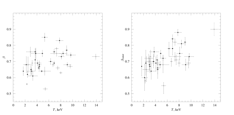
Figure 2.— Correlation of $\beta$ with temperature. The values of $\beta$ are derived from the global fit and from the fit in the radial range $0.3r_{180}<r<1.5r_{180}$ in the left and right panels, respectively. Filled and open circles correspond to cooling flow and non cooling flow clusters, respectively.

Table 2Surface Brightness Fitting and Gas Mass Results

Name	$\beta_{\rm outer}^{\rm(a)}$	$\beta_{rc,\rm out}^{\rm(b)}$	$\beta^{\rm(c)}$	$r_{c}^{\rm(c)}$	$R_{2000}^{\rm(d)}$	$R_{1000}^{\rm(d)}$	$\delta\beta_{\rm azi}^{\rm(e)}$	$\delta M_{\rm azi}^{\rm(f)}$
2A0335	$0.68\pm 0.03$	$0.65$	$0.65\pm 0.03$	($0.08\pm 0.08$)	$1.33\pm 0.03$	$1.88\pm 0.07$	0.04	0.09
A133	$0.76\pm 0.03$	$0.78$	$0.75\pm 0.03$	($0.37\pm 0.05$)	$1.36\pm 0.03$	$1.93\pm 0.09$	0.09	0.16
A1413	$0.70\pm 0.02$	$0.67$	$0.68\pm 0.01$	($0.20\pm 0.01$)	$1.66\pm 0.10$	$2.43\pm 0.15$	0.08	0.17
A1651	$0.78\pm 0.04$	$0.75$	$0.70\pm 0.02$	($0.26\pm 0.03$)	$1.70\pm 0.06$	$2.41\pm 0.15$	0.23	0.18
A1689	$0.82\pm 0.02$	$0.79$	$0.77\pm 0.03$	($0.27\pm 0.05$)	$1.76\pm 0.07$	$2.46\pm 0.15$	0.00	0.14
A1795	$0.88\pm 0.02$	$0.89$	$0.83\pm 0.02$	($0.39\pm 0.02$)	$1.73\pm 0.01$	$2.37\pm 0.05$	0.12	0.09
A2029	$0.68\pm 0.03$	$0.67$	$0.68\pm 0.01$	($0.28\pm 0.03$)	$2.02\pm 0.05$	$2.90\pm 0.12$	0.00	0.12
A2052	$0.67\pm 0.04$	$0.65$	$0.64\pm 0.02$	($0.10\pm 0.05$)	$1.19\pm 0.06$	$1.77\pm 0.12$	0.04	0.12
A2063	$0.69\pm 0.04$	$0.68$	$0.69\pm 0.02$	($0.22\pm 0.02$)	$1.19\pm 0.05$	$1.71\pm 0.14$	0.11	0.14
A21	$0.68\pm 0.05$	$0.69$	$0.64\pm 0.02$	($0.31\pm 0.03$)	$1.42\pm 0.08$	$2.08\pm 0.17$	0.00	0.15
A2142	$0.73\pm 0.02$	$0.73$	$0.74\pm 0.01$	($0.42\pm 0.03$)	$2.29\pm 0.03$	$3.23\pm 0.10$	0.05	0.11
A2163	$0.90\pm 0.04$	$0.89$	$0.73\pm 0.02$	($0.42\pm 0.02$)	$2.48\pm 0.09$	$3.42\pm 0.17$	0.00	0.23
A2199	$0.68\pm 0.02$	$0.67$	$0.64\pm 0.01$	($0.14\pm 0.01$)	$1.41\pm 0.01$	$2.02\pm 0.02$	0.07	0.07
A2218	$0.71\pm 0.03$	$0.70$	$0.66\pm 0.01$	($0.24\pm 0.01$)	$1.59\pm 0.05$	$2.33\pm 0.08$	0.07	0.15
A2255	$0.73\pm 0.03$	$0.77$	$0.75\pm 0.02$	($0.55\pm 0.02$)	$1.70\pm 0.05$	$2.53\pm 0.10$	0.18	0.06
A2256	$0.82\pm 0.02$	$0.82$	$0.78\pm 0.01$	($0.46\pm 0.01$)	$1.88\pm 0.01$	$2.69\pm 0.03$	0.05	0.08
A2382	$0.72\pm 0.03$	$0.81$	$0.76\pm 0.03$	($0.47\pm 0.03$)	$1.13\pm 0.05$	$1.73\pm 0.10$	0.04	0.22
A2462	$0.65\pm 0.08$	$0.67$	$0.68\pm 0.05$	($0.22\pm 0.04$)	$0.86\pm 0.11$	$1.30\pm 0.23$	0.00	0.23
A2597	$0.66\pm 0.04$	$0.67$	$0.68\pm 0.02$	($0.18\pm 0.04$)	$1.32\pm 0.09$	$1.93\pm 0.14$	0.13	0.15
A2657	$0.70\pm 0.03$	$0.75$	$0.76\pm 0.02$	($0.37\pm 0.02$)	$1.22\pm 0.03$	$1.76\pm 0.07$	0.07	0.11
A2717	$0.60\pm 0.08$	$0.67$	$0.68\pm 0.05$	($0.07\pm 0.08$)	$0.84\pm 0.05$	$1.18\pm 0.12$	0.00	0.13
A3112	$0.71\pm 0.03$	$0.69$	$0.63\pm 0.02$	($0.12\pm 0.08$)	$1.53\pm 0.05$	$2.17\pm 0.13$	0.02	0.12
A3301	$0.70\pm 0.04$	$0.72$	$0.64\pm 0.03$	($0.29\pm 0.03$)	$1.04\pm 0.06$	$1.58\pm 0.12$	0.09	0.15
A3391	$0.55\pm 0.03$	$0.54$	$0.53\pm 0.01$	($0.21\pm 0.01$)	$1.41\pm 0.06$	$2.25\pm 0.18$	0.08	0.06
A3571	$0.78\pm 0.04$	$0.77$	$0.69\pm 0.01$	($0.27\pm 0.02$)	$1.87\pm 0.06$	$2.62\pm 0.11$	0.04	0.07
A400	$0.58\pm 0.02$	$0.58$	$0.56\pm 0.01$	($0.18\pm 0.01$)	$0.92\pm 0.02$	$1.45\pm 0.06$	0.01	0.11
A401	$0.69\pm 0.02$	$0.68$	$0.63\pm 0.01$	($0.27\pm 0.01$)	$2.08\pm 0.04$	$2.98\pm 0.13$	0.06	0.17
A4038	$0.64\pm 0.05$	$0.63$	$0.61\pm 0.03$	($0.16\pm 0.06$)	$1.15\pm 0.07$	$1.64\pm 0.11$	0.00	0.15
A4059	$0.65\pm 0.05$	$0.66$	$0.67\pm 0.02$	($0.22\pm 0.05$)	$1.30\pm 0.06$	$1.93\pm 0.12$	0.05	0.14
A478	$0.81\pm 0.02$	$0.80$	$0.75\pm 0.01$	($0.31\pm 0.03$)	$1.94\pm 0.03$	$2.70\pm 0.10$	0.07	0.09
A496	$0.75\pm 0.02$	$0.74$	$0.70\pm 0.02$	($0.25\pm 0.02$)	$1.43\pm 0.03$	$1.99\pm 0.10$	0.00	0.08
A539	$0.73\pm 0.04$	$0.74$	$0.69\pm 0.02$	($0.25\pm 0.01$)	$1.06\pm 0.05$	$1.52\pm 0.10$	0.32	0.23
A644	$0.75\pm 0.04$	$0.73$	$0.73\pm 0.02$	($0.24\pm 0.02$)	$1.69\pm 0.05$	$2.38\pm 0.14$	0.00	0.13
A85	$0.84\pm 0.02$	$0.86$	$0.76\pm 0.02$	($0.40\pm 0.02$)	$1.81\pm 0.03$	$2.51\pm 0.09$	0.11	0.18
AWM4	$0.69\pm 0.08$	$0.67$	$0.62\pm 0.02$	($0.11\pm 0.01$)	$0.75\pm 0.05$	$1.17\pm 0.11$	0.00	0.14
A780	$0.71\pm 0.03$	$0.69$	$0.66\pm 0.01$	($0.12\pm 0.03$)	$1.48\pm 0.02$	$2.02\pm 0.08$	0.19	0.13
MKW3S	$0.70\pm 0.04$	$0.72$	$0.71\pm 0.07$	($0.30\pm 0.10$)	$1.22\pm 0.06$	$1.76\pm 0.15$	0.00	0.11
MKW4	$0.67\pm 0.06$	$0.67$	$0.64\pm 0.03$	($0.18\pm 0.02$)	$0.71\pm 0.05$	$1.11\pm 0.09$	0.15	0.12
Tri Aus	$0.69\pm 0.03$	$0.69$	$0.67\pm 0.01$	($0.36\pm 0.02$)	$2.29\pm 0.04$	$3.22\pm 0.11$	0.07	0.11

^(a) — results of the fit for the radial range $0.3r_{180}<r<1.5r_{180}$ with core-radius fixed at $0.1r_{180}$. ^(b) — $\beta$ parameter in the $0.3r_{180}<r<1.5r_{180}$ range with core radius fixed at a value derived from the fit for the entire radial range. Uncertainties in $\beta_{rc,\rm out}$ and in $\beta_{\rm outer}$ are similar. ^(c) — results over the entire radial range (excluding the cooling flow); core-radius values for cooling flow clusters are given in parentheses. ^(d) — radius of the mean gas overdensity $\Delta=1000$ and 2000 relative to the background baryon density. ^(e) — Azimuthal rms variations of $\beta_{\rm outer}$ in excess of the statistical variations. ^(f) — Azimuthal relative rms variations of the gas mass within $R_{1000}$, including statistical noise.

4.2. Surface Brightness Slope

For comparison with previous studies, the results of fitting the beta-model to azimuthally averaged surface brightness profiles in the radius range $2\,r_{\rm cool}$–$1.5\,r_{180}(T)$ for cooling flow, and $0$–$1.5\,r_{180}(T)$ for non-cooling flow clusters, are presented in Table 2. For cooling flow clusters, the best fit values of core radius are often comparable to the radius of the excluded region; therefore, the core radii cannot be reliably measured for those clusters. The $\beta$-parameter, on the other hand, is measured very accurately, and the $\beta$-model fits generally provide a very good description of the data (see examples in Fig. 1). The best-fit values of $\beta$ are plotted versus the cluster temperature in Fig. 2. Similarly to Jones & Forman (1998), we find that values of $\beta$ are distributed over a narrow range $0.7\pm 0.1$ for most clusters. However, the distributions in our and Jones & Forman samples are slightly offset. Jones & Forman find the average value $\langle\beta\rangle=0.6$, while all but two our clusters have $\beta>0.6$. This difference is attributable in part to different techniques of excising the cooling flows; but also, because of the larger field of view and lower background, ROSAT data trace the surface brightness to larger radius where the profiles often steepen (see below).

Unlike, for example, clusters in the Jones & Forman (1984, 1999) sample, there are no hints of a correlation of $\beta$ with cluster temperature (left panel in Fig. 2). A careful examination shows that the previously reported correlation of $\beta$ with temperature is due to small values of $\beta\sim 0.5$ for cool clusters with $T\sim 3$ keV, for which we find significantly steeper profiles. Again, a likely explanation for this discrepancy is the incomplete removal of cooling flows in the earlier studies; a cooling flow, if not accounted for completely, biases $r_{c}$ and $\beta$ low.

To determine the slope of the surface brightness profiles at large radii, we fit the profiles in the same range of radii in virial coordinates, $0.3\,r_{180}(T)<r<1.5\,r_{180}(T)$. With this choice of radii, clusters of different temperatures are compared in the same range of physical coordinates. The core radius cannot be determined from this fit, and so we fixed its value at either $0.1\,r_{180}$ or the value derived from the fit for the entire radial range. Because the value for core-radius is typically much smaller than the inner radius of the data, these modelings are equivalent to fitting the power law relation, $S\propto r^{-6\beta+1}$. The values of $\beta_{\rm outer}$ are listed in Table 2 and plotted versus cluster temperature in Fig. 2.

The slopes in the outer parts in many clusters are slightly steeper than those given by the $\beta$-model. The extreme case is A2163, where $\beta$ changes by 0.17. The surface brightness profile of this cluster shows a clear steepening at $r>0.3\,r_{180}(T)$ (Fig. 2). Although this cluster is probably a merger (see discussion in Markevitch et al. 1996), the same steepening in the surface brightness is seen in all but one of the $60^{\circ}$ sectors. However, the typical change of $\beta$ in the outer parts is much smaller, $\Delta\beta\approx 0.05$, and only marginally significant in most clusters. Thus, a strong steepening of the gas density distribution at large radius suggested by Bartelmann & Steinmetz (1996) is excluded.

There is some indication of a positive correlation of $\beta_{\rm outer}$ with temperature. This is mainly due to a group of 5 hot, $T=6-10$ keV, clusters with $\beta_{\rm outer}>0.8$, and a strong steepening of the surface brightness profile in the hottest cluster A2163. However, as is seen from Fig. 2, the possible change of slope is well within the scatter at high temperatures. In any case, the change of slope is small, from $\beta\approx 0.67$ for 3 keV clusters to $\beta\approx 0.8-0.85$ for 10 keV clusters.

4.3. Azimuthal Variations of the Surface Brightness

Cluster X-ray surface brightness is often described by a radial profile (as in the previous sections). It is important to determine how accurate this description is in the outer region. We divide the clusters into sectors 0^∘–60^∘, …, 300^∘–360^∘, and determine $\beta_{\rm outer}$ in the radial range $0.3\,r_{180}(T)<r<1.5\,r_{180}(T)$ in each sector separately. Azimuthal variations of $\beta_{\rm outer}$ would indicate an asymmetric cluster.

Azimuthal variations of $\beta$ in the outer part of A2029 and A1795.

The sample appears to have clusters from very regular ones, such as A2029, to those which display statistically significant azimuthal variations of the slope, such as A1795 (Fig. 4.3). However, the amplitude of variations is typically not very large. The azimuthal rms variations of $\beta_{\rm outer}$ in excess of the statistical noise level are listed for all clusters in Table 2. In most cases, these variations are below 0.1, and in many cases are dominated by a strong deviation in just one sector. We conclude that the azimuthal averaging of the surface brightness in the cluster outer parts can be justified. We will return to the issue of azimuthal averaging in the discussion of gas mass distribution below.

5. Gas Mass Distribution

The X-ray surface brightness distribution in clusters receives much attention because it can be rather precisely converted to the distribution of hot gas. Determination of the gas mass distribution is also a goal of our study. Below we briefly review techniques used to derive the gas density and present the results for our sample.

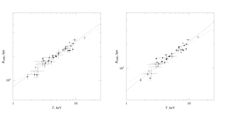
Figure 3.— Correlation of $R_{1000}$ and $R_{2000}$ with temperature. Dashed lines show the best power law fit, $R_{1000}\propto T^{0.57}$ and $R_{2000}\propto T^{0.61}$, while the dotted lines show $R\propto T^{0.5}$ fits. Filled and open circles correspond to cooling flow and non cooling flow clusters, respectively.

5.1. Conversion of Surface Brightness to Gas Mass

Under the assumption of spherical symmetry, the observed surface brightness profile can be converted to the emissivity profile. The latter is then easily converted to the gas density profile, because the X-ray emissivity of hot, homogeneous plasma is proportional to the square of the density and, in the soft X-ray band, depends only very weakly on temperature (e.g., Fabricant, Lecar, & Gorenstein 1980, and §6.2 below).

There are two main techniques to convert the observed surface brightness profile to the emissivity profile under the assumption of spherical symmetry. The first method is to fit an analytical function to the surface brightness profile $S(r)$ and then deproject the fit using the inverse Abell integral (e.g., Sarazin 1986). For the $\beta$-model surface brightness fit (eq. 1), the conversion is particularly simple (Cavaliere & Fusco-Femiano 1976, Sarazin 1986).

The second widely used technique is the direct deprojection of the data without using an analytical model (Fabian et al. 1981, Kriss, Cioffi, & Canizares 1983). Briefly, one assumes that the emissivity is uniform within spherical shells corresponding to the surface brightness profile annuli. The contribution of the outer shells to the flux in each annuli can be subtracted, and the emissivity in the shell calculated, using simple geometrical considerations. This method has an important advantage over the $\beta$-fit, in that no functional form of the gas distribution is assumed and realistic statistical uncertainties at each radius are obtained. Although we generally find very little difference between the deprojection and $\beta$-fit methods, we use the deprojection technique as the preferred one.

Once the distribution of emissivity (in units of flux per volume) is known, it can be converted to the distribution of gas mass as follows. The emissivity is multiplied by the volume of the spherical shell to obtain the total flux from this shell. Assuming that the gas temperature is constant at all radii, we use the Raymond & Smith (1977) spectral code to find the conversion coefficient between the flux and the emission measure integral, $E=\int n_{e}n_{p}\,dV$, given the plasma temperature, heavy metal abundance, cluster redshift, and Galactic absorption. Metal abundance has virtually no effect on the derived gas mass at high temperatures, which is the case for our clusters; we assume that it is 0.3 of the Solar value for all clusters. For this metal abundance, $n_{e}/n_{p}=1.17$, and the gas density is $\rho_{g}=1.35\,m_{p}n_{p}$. The gas mass in the shell is $m_{g}=m_{p}(1.56\,E\,V)^{1/2}$, where $V$ is the volume of the shell. Given the observed flux, the derived gas mass scales with distance to the cluster as $d^{5/2}$.

5.2. Correlation of the Baryon Overdensity Radius with Temperature

As was pointed out in §1, simple theory predicts a tight correlation between the radius at a fixed baryon overdensity relative to the background density of baryons and the temperature in the form $R\propto T^{0.5}$. Since most baryons in clusters are in the form of hot gas, and the gas mass is easily measured from the X-ray data, this correlation can be tested observationally.

We use the deprojection technique to determine the enclosed gas mass as a function of radius. The baryon overdensity is calculated as the ratio of the enclosed mass and $(4\pi/3)\rho_{0}R^{3}(1+z)^{3}$, where $\rho_{0}$ is the present day background density of baryons derived from primordial nucleosynthesis, and $z$ is the cluster redshift. We adopt the value $\rho_{0}=2.85\times 10^{9}$ $M_{\odot}$ Mpc^-3 (Walker et al. 1991); a different value of the background baryon density (e.g., a recent determination by Burles & Tytler 1998) would have no effect on our results except for scaling the reported overdensities.

Previous studies of the baryonic contents in clusters indicated that baryons contribute $\sim 15-20\%$ of the total cluster mass (for $h=0.5$); if this ratio is representative of the Universe as a whole, it corresponds to a cosmological density parameter $\Omega_{0}=0.2-0.3$ (White et al. 1993, David et al. 1995, Evrard 1997). With this range for $\Omega_{0}$, the two commonly referenced values of the dark matter overdensity $\delta=180$ and 500 relative to the critical density correspond to gas overdensities $\Delta_{g}=600-1000$ and 1500–2500, respectively. Therefore, we determine the radii at which the mean enclosed hot gas density is 1000 and 2000 above the baryon background; these radii are denoted $R_{1000}$ and $R_{2000}$ hereafter.

For a wide range of gas temperatures, from 1.5 to 10 keV, the gas mass corresponding to the fixed ROSAT flux changes by only 4% if metal abundance is $a=0.3$ Solar, and by 10%, if $a=0.5$. The corresponding variations of the gas overdensity radius are approximately $2\%$ and 5%. Therefore, the values of $R_{1000}$ and $R_{2000}$, as derived from the ROSAT data, are practically independent of the gas temperature.

The measured radii $R_{1000}$ and $R_{2000}$ are plotted versus cluster temperature in Fig. 3. Note that $R$ and $T$ are measured essentially independently, as opposed, for example, to the baryon fraction or total mass that involves mass estimates that use the gas temperature. The correlation is very tight and close to the theoretically expected $R\propto T^{0.5}$. Note that even A3391, the cluster with an anomalously flat surface brightness profile, is quite close to the observed correlation. We fit power laws to the $R-T$ relation using the bisector modification of the linear regression algorithm that allows for intrinsic scatter and non-uniform measurement errors, and treats both variables symmetrically (Akritas & Bershady 1996 and references therein). The confidence intervals were determined using bootstrap resampling (e.g., Press et al. 1992). The best fit relations are

$$\lg R_{1000} = (0.569\pm 0.043)\,\lg T+2.918$$

$$\lg R_{2000} = (0.615\pm 0.042)\,\lg T+2.720,$$ (2)

where radii are in kpc and temperatures are in keV, and uncertainties are $68\%$ confidence. For any given temperature, the average scatter in $R_{1000}$ is only 6.5%, and $\sim 7\%$ for $R_{2000}$. This is comparable to the scatter of the dark matter overdensity radius $r_{500}$ in simulated clusters (Evrard et al. 1996). Even though the best fit slopes formally deviate from the expected value of 0.5 by $2-3\sigma$, the difference between the best fit and the $R\propto T^{0.5}$ relation is within the scatter in the data (Fig. 3).

Figure 4.— Raw and scaled gas density profiles. For readability, density profiles are calculated from the $\beta$-model fits instead of our preferred deprojection technique.

A tight correlation of the baryon overdensity radius with temperature suggests that the gas density profiles in the outer parts of clusters are similar, when appropriately scaled. Figure 4 shows the gas density profiles plotted as a function of radius in Mpc, in units of $r_{180}(T)$, and in units of $R_{1000}$. No density scaling was applied. As expected, density profiles display a large scatter if no radius scaling is applied, since we are comparing systems of widely different masses. The density scatter at large radius becomes small (the entire range is $\approx\pm 40\%$) when radii are scaled to $r_{180}(T)$. This scatter is close to that of the dark matter density in simulated clusters. The scatter is particularly small when profiles are scaled to the overdensity radius $R_{1000}$. One can argue that in this case, the scatter is artificially suppressed because the scaling depends on the density. However, the scatter remains small over a rather wide radial range; also, the same critique applies when dark matter profiles of simulated clusters are plotted in virial coordinates.

To conclude, gas density profiles show a high degree of similarity, both in terms of enclosed mass and shape, when the radius is scaled to either the virial radius estimated from the gas temperature or the fixed gas overdensity radius. In the next section, we discuss some uncertainties which affect the measurement of the gas mass distribution.

6. Discussion of Gas Mass Uncertainties

6.1. Sample Selection and Spherical Symmetry

To calculate gas mass from the observed X-ray surface brightness, we, and most other studies, assume that the cluster is spherically symmetric. It is desirable to check that this assumption is adequate. If the substructure had a strong effect on the derived gas mass, the mass calculated using surface brightness profiles in different cluster sectors would be substantially different when the substructure is seen in projection. Because of random orientations, substructure in projection occurs more often than along the line of sight. Therefore, the azimuthal variations of the gas mass can be used to place limits on the 3-dimensional deviations from the spherical symmetry. To look for this effect, we calculated gas masses using surface brightness profiles in six sectors in all clusters. The rms azimuthal gas mass variations within $R_{1000}$ are listed in Table 2. For most clusters, these variations are on the level of $\sim 10-15\%$, including statistical scatter. Since we find that mass variations in projection are small, this indicates that they also are small in three-dimensional space.

It can be argued that only small azimuthal mass variations are found because clusters with substructure were excluded from the sample. Moreover, such selection might lead to a preferential selection of clusters having substructure along the line of sight which is invisible in the images. As a result, our gas distribution measurements might be seriously biased, because we do not average over different cluster orientations.

These arguments are countered by the following considerations. We excluded only three cooling flow clusters, Cyg-A, A3558, and A1763, on the basis of strong substructure, compared to 25 such clusters in the sample (Table 1). Therefore, our cooling flow subsample, which comprises two thirds of the total sample, should be unbiased with respect to substructure selection. Since there is no obvious difference between cooling and non-cooling flow clusters either in terms of gas mass (Fig. 3) or surface brightness fits (Fig. 2), our subsample of non-cooling flow clusters also is unlikely to have significant substructure along the line of sight.

6.2. Temperature Structure

ASCA measurements suggest that, at least in hot clusters, the gas temperature gradually declines with radius reaching $\sim 0.5$ of the average value at $r=0.5\,r_{180}$ (Markevitch et al. 1998). Because of strong line emission, calculation of the gas density from ROSAT flux is uncertain for cool clusters, if precise temperatures and metal abundances are unknown. If such cool ($T\sim 2$ keV) clusters have declining temperature profiles, our gas masses will be affected, because we assume isothermality. Fortunately, the effect is not very strong. We tested this by simulating the $T=0.5$ keV Raymond-Smith plasma with heavy metal abundance, $a$, in the range 0.1–0.5 of the Solar value, and converting the predicted ROSAT PSPC flux in the 0.5–2 keV band back to gas mass using the $T=2$ keV, $a=0.3$ spectral model. The mass was underestimated by 20% for $a=0.1$ and overestimated by $35\%$ for $a=0.5$. For the input spectrum with $T=1$ keV, the mass error was in the range $\pm 15\%$. The effect of temperature decline on the enclosed gas mass is smaller, because a significant mass fraction is contained within the inner, hotter regions. The error in the gas overdensity radius determination is still smaller because overdensity is a very strong function of radius (for example, $\Delta_{g}\propto r^{-2}$ for $\beta=2/3$).

6.3. Cooling Flows

The presence of a cooling flow leads to an overestimate of the gas density near the cluster center, if one assumes that the gas is single-phase and isothermal. However, the enclosed gas mass at large radius is little affected, because most of gas mass lies at large radii. For example, in A1795, the cluster with one of the strongest cooling flows, only 2.7% of the gas mass inside $R_{1000}$ is within the cooling radius and 9% of the mass is within $2\,r_{\rm cool}$, if one assumes that the cooling flow is single-phase and isothermal. Even if the mass within $2\,r_{\rm cool}$ is overestimated by 100% because of these incorrect assumptions, the total gas mass is overestimated by only 10%, and $R_{1000}$ is overestimated by only 3%. The true errors are likely to be smaller.

The presence of a cooling flow also leads to an underestimate of the emission-weighted temperature (underestimation here is relative to the absence of radiative cooling, the assumption usually made in theory and simulations). For example, Markevitch et al. (1998) find that in several clusters, the temperature increases by up to 30% when the cooling flow is excised. This temperature error produces almost no to errors in gas masses, but can introduce an additional scatter in the $R-T$ correlation, or in the gas density profiles scaled to $r_{180}(T)$. We used temperatures from Markevitch et al. for which cooling flows were excised, for all clusters with strong cooling flows, except 2A0335 and A1689. Allen and Fabian (1998) find that the temperature increase in A1689 when the cooling flow is modeled as an additional spectral component is small, $\sim 5\%$. Cooling flows in other clusters in our sample are not very strong, and simple emission-weighted temperatures should be sufficiently accurate.

7. Discussion

7.1. Applicability of the $\beta$-model

We have found above that the slope of the surface brightness profile in the outer part of clusters [$0.3\,r_{180}-r_{180}$] is slightly steeper than the slope of the $\beta$-model fit in the entire radial range (excluding the cooling flow region). Thus, the $\beta$-model does not describe the gas distribution precisely. However, deviations from the $\beta$-model are small and do not lead to significant errors in the total mass or gas mass. Consider the extreme case of A2163, where the global $\beta$-value is 0.73 but beyond a radius of $0.3\,r_{180}(T)$, the profile slope steepens to $\beta=0.9$. Such a change of $\beta$ leads to a 24% increase of the total mass calculated from the hydrostatic equilibrium equation; this is smaller than other uncertainties (Markevitch et al. 1996). The gas masses within $R_{1000}$ calculated from the global $\beta$-model and from the exact surface brightness profile differ by 20%. In most clusters, where $\beta$ typically changes by $\approx 0.05$, the effect on the total and gas mass is much smaller.

7.2. $R-T$: The First “Proper” Scaling for Baryons

The scaling relations involving hot gas in clusters established previously show significant deviations from the theoretically expected relations. The most notable example is the luminosity-temperature correlation. From the virial theorem relation $M_{\rm tot}\propto T^{3/2}$, and the assumptions of constant baryon fraction and self-similarity of clusters, one expects $L_{x}\propto T^{2}$ while the observed relation is closer to $L_{x}\propto T^{3}$ (David et al. 1993). The current consensus is that additional physics, such as preheating of the intergalactic medium or the feedback from galaxy winds/supernovae or shock heating of the IGM has important effects on the X-ray luminosities (see Cavaliere, Menci & Tozzi 1997 and references therein). These processes are still uncertain, and for example, prevent the use of the evolution of the cluster luminosity function as a cosmological probe.

Another example of the deviations of cluster baryon scaling from theoretical expectations is the relation between the cluster size at a fixed X-ray surface brightness and temperature (Mohr & Evrard 1997). Mohr & Evrard find $R_{I}\propto T^{0.9\pm 0.1}$ from the observations, while their simulated clusters show $R_{I}\propto T^{0.7}$. After inclusion of feedback from galaxy winds to the simulations, Mohr & Evrard were able to reproduce the observed size-temperature relation. Note that the surface brightness threshold used by Mohr & Evrard was selected at a high level, so that the derived size $R_{I}$ was only $\approx 0.3$ of the cluster virial radius.

The scaling between the radius of a fixed gas overdensity and temperature, $R\approx\mathrm{const}\times T^{1/2}$, presented here is, to our knowledge, the first observed scaling involving only cluster baryons that is easily understandable theoretically (§1). The crucial difference between the luminosity-temperature and Mohr & Evrdard’s size-temperature relation and our scaling is that we use cluster properties at large radius, where most of the mass is located, while the $L-T$ and $R_{I}-T$ relations are based on properties of the inner cluster regions. Our findings thus suggest that any processes required to explain the observed $L-T$ and $R_{I}-T$ relations affect only central cluster parts and are not important for the gas distribution at large radii.

7.3. Limit on the Variations in the Baryon Fraction

Simulations predict that the total mass within a radius of fixed overdensity scales as $M_{\rm tot}\propto T^{3/2}$ (Evrard et al. 1996). Our observed scaling between the gas overdensity radius and $T$ is consistent with $R\propto T^{1/2}$, or equivalently $M_{\rm gas}\propto T^{3/2}$. Therefore, if the simulations are correct, $M_{\rm gas}/M_{\rm tot}$ does not depend on the cluster temperature. Since hot gas is the dominant component of baryons in clusters, the baryon fraction within a radius of fixed overdensity is constant for all clusters. To be more precise, the best-fit relation $R_{1000}\propto T^{0.57}$ corresponds to a slowly varying gas fraction $M_{\rm gas}/M_{\rm tot}=T^{0.2}$. However, the stellar contribution can reduce this trend, because stars contribute a greater fraction of the baryon mass in low-temperature clusters (David et al. 1990, David 1997).

The small observed scatter around the mean $R-T$ relation can be used to place limits on the variations of the baryon fraction between clusters of similar temperature. At large radius, the mean gas overdensity is $\Delta_{g}\propto r^{-3\beta}$. Therefore, the $\sim 7\%$ observed scatter in radius at the given $\Delta$ corresponds to a $3\beta\times 7\%$ scatter in overdensity at the given radius. Assuming that the total cluster mass is uniquely characterized by the temperature, the scatter in $M_{\rm gas}/M_{\rm tot}$ is 14–18%, including the measurement uncertainties. The small scatter indicates that the baryon fraction in clusters is indeed universal. There is also an intrinsic scatter in the $M_{\rm tot}-T$ relation, which is 8%–15% in simulated clusters (Evrard et al. 1996); if the deviations of the total mass and gas mass from the average value expected for the given temperature are not anti-correlated, the scatter of the baryon fraction is reduced still further. Thus, our results provide further observational support for measurements of $\Omega_{0}$ from the baryon fraction in clusters and the global density of baryons derived from primordial nucleosynthesis.

7.4. Similarity of Gas Density Profiles

The gas density profiles plotted in virial coordinates, i.e., radius scaled by either $r_{180}(T)$ or $R_{1000}$, are very similar, both in slope and normalization (Fig. 4). The similarity of the gas density slopes in the outer parts of clusters also is evident from the relatively small scatter of $\beta$-values in Fig. 2. Most clusters have $0.65<\beta_{\rm outer}<0.85$, which corresponds to gas density falling with radius between $r^{-1.95}$ and $r^{-2.55}$.

The average gas density, $\rho_{\rm g}\sim r^{-2.25}$, is significantly more shallow than the universal density profile of the dark matter halos found in numerical simulations, $\rho_{\rm dm}\sim r^{-2.7}$ between $0.3\,r_{180}$ and $r_{180}$ (Navarro et al. 1995). Moreover, if gas in this radial range is in hydrostatic equilibrium and isothermal, a power law function of gas density with radius implies $\rho_{\rm dm}\sim r^{-2}$. Under the hydrostatic equilibrium assumption, the average gas polytropic index $\gamma\sim 1.3$, or equivalently $T\propto r^{-0.7}$, is required for the total mass to follow the Navarro et al. distribution. Interestingly, this is quite close to the temperature profile observed in many clusters within $0.5\,r_{180}$ (Markevitch et al. 1998).

7.5. Comparison with Other Works

After this paper was submitted, we learned about works of Mohr, Mathiesen & Evrard (1999) and Ettori & Fabian (1999) who also studied the hot gas distribution in large cluster samples. We briefly discuss some aspects of these works that are in common with our study.

Both Mohr et al. and Ettori & Fabian derive cluster $\beta$’s from a global fit. Ettori & Fabian exclude central 200 kpc in the cooling flow clusters; they find the global $\beta$’s in the range 0.6–0.8, in agreement with our results. Mohr et al. fit the cooling flow region with an additional $\beta$-model component, but force the same $\beta$ for the cluster and cooling flow components. Their values of $\beta$ for cooling flow clusters are often flatter than ours (e.g., they derive $\beta=0.66\pm 0.03$ for A85, while our value is 0.76); most likely, this is due to the difference in fitting procedures.

Mohr et al. find a tight correlation of the cluster temperature with the hot gas mass within $r_{500}$ (estimated as $r_{500}=C\times T^{1/2}$) in the form $M_{\rm gas}\propto T^{1.98\pm 0.18}$. Because the gas mass and gas overdensity radius are related as $M_{\rm gas}={\rm const}\times R^{3}$, the $M_{\rm gas}-T$ and our $R_{1000}-T$ correlations are almost equivalent. However, our correlation corresponds to a flatter $M_{\rm gas}-T$ relation, $M\propto T^{1.71\pm 0.13}$, closer to the theoretically expected slope of 1.5. There is an important difference of our and Mohr et al. approaches. While in our method, $R_{1000}$ and $T$ are measured essentially independently, the Mohr et al. measurement of the gas mass does depend on $T$ through $r_{500}$. Since $r_{500}\propto T^{1/2}$ and typically $M_{\rm gas}(<r)\sim r$, their method would find $M_{\rm gas}\propto T^{1/2}$ even if gas profiles of all clusters are the same. This effect may introduce a bias which is responsible for a slightly steeper $M_{\rm gas}-T$ relation in Mohr et al.

Mohr et al. and Ettori & Fabian (for low-redshift clusters) find that the values of gas fraction in hot clusters are distributed in a relatively narrow range, $f_{\rm gas}\sim 0.2\pm 0.04$. Our tight correlation of $R_{1000}$ and $T$ also implies a low, $\sim 15\%$ scatter in $f_{\rm gas}$ (see above).

8. Summary

We have carried out a detailed analysis of the surface brightness distributions of a sample of 25 cooling flow clusters and 14 non-cooling flow clusters. Since the bulk of the cluster gas mass, and hence the luminous cluster baryons, reside at large radii, we have focussed on the properties of the gas profile at large radii

The cluster profiles, from $0.3r_{180}$ to $r_{180}$ can be accurately characterized as a single power law with $\beta=0.65-0.85$. These outer profiles are steeper by about 0.05 in $\beta$ on average than profiles fit using the entire surface brightness profile (but excluding the cooling flow region). This indicates that the $\beta$-model does not describe the surface brightness profiles precisely.

The previously reported correlation of increasing $\beta$ with increasing temperature (steepening profiles with increasing temperatures) is only weakly present in our data. This difference arises primarily because the low ROSAT background allows us to detect clusters to near the virial radius where they exhibit more similar profiles than in the central part, often dominated by the cooling flow.

We find a very precise correlation of the radius, corresponding to a fixed baryon overdensity, with gas temperature which is consistent with that theoretically predicted from the virial theorem. For example, the radius at which the mean baryon overdensity is 1000 is best fit as a function of temperature as $R_{1000}\propto T^{0.57\pm 0.04}$ and is consistent within the scatter with the theoretically expected relation $R\propto T^{0.5}$.

The observed scatter in the correlation of $R_{1000}$ vs. $T$ is small. Quantitatively, for any given temperature the average scatter in $R_{1000}$ is approximately 7%. This corresponds to a scatter in $M_{\rm gas}/M_{\rm tot}$ at the same radius of less than 20%, which includes any intrinsic variation as well as measurement errors.

At large radii, cluster gas density distributions are remarkably similar when scaled to the cluster virial radius ($r_{180}$) and they are significantly shallower than the universal profile of dark matter density found in simulations (Navarro et al. 1995). However, for gas in hydrostatic equilibrium, the temperature profile found by Markevitch et al. (1998) combined with the gas density profiles observed for our sample imply a dark matter distribution quite similar to the universal one found in numerical simulations.