Destriping of Polarized Data in a CMB Mission with a Circular Scanning Strategy

Abstract

A major problem in Cosmic Microwave Background (CMB) anisotropy mapping, especially in a total-power mode, is the presence of low-frequency noise in the data streams. If unproperly processed, such low-frequency noise leads to striping in the maps. To deal with this problem, solutions have already been found for mapping the CMB temperature fluctuations but no solution has yet been proposed for the measurement of CMB polarization. Complications arise due to the scan-dependent orientation of the measured polarization. In this paper, we investigate a method for building temperature and polarization maps with minimal striping effects in the case of a circular scanning strategy mission such as the Planck mission.

1 Introduction

Theoretical studies of the CMB have shown that the accurate measurement of the CMB anisotropy spectrum $C^{T}_{\ell}$ with future space missions such as Planck will allow for tests of cosmological scenarios and the determination of cosmological parameters with unprecedented accuracy. Nevertheless, some near degeneracies between sets of cosmological parameters yield very similar CMB temperature anisotropy spectra. The measurement of the CMB polarization and the computation of its power spectrum Seljak (1996); Zaldarriaga (1998) may lift to some extent some of these degeneracies. It will also provide additional information on the reionization epoch and on the presence of tensor perturbations, and may also help in the identification and removal of polarized astrophysical foregrounds Kinney (1998); Kamionkowski (1998); Prunet and Lazarian (1999).

A successful measurement of the CMB polarization stands as an observational challenge; the expected polarization level is of the order of $10\%$ of the level of temperature fluctuations ($\Delta T/T\simeq 10^{-5}$). Efforts have thus gone into developing techniques to reduce or eliminate spurious non-astronomical signals and instrumental noise which could otherwise easily wipe out real polarization signals. In a previous paper Couchot et al. (1999), we have shown how to configure the polarimeters in the focal plane in order to minimize the errors on the measurement of the Stokes parameters. In this paper, we address the problem of low frequency noise.

Low frequency noise in the data streams can arise due to a wide range of physical processes connected to the detection of radiation. $1/f$ noise in the electronics, gain instabilities, and temperature fluctuations of instrument parts radiatively coupled to the detectors, all produce low frequency drifts of the detector outputs.

Figure 1: The power spectrum of the K34 bolometer from Caltech, the same type of bolometer planned to be used on the Planck mission. The measurement was performed at the SYMBOL test bench at I.A.S., Orsay (supplied by Michel Piat). The knee frequency of this spectrum is $\sim 0.014$ Hz and the planned spin frequency for Planck is $0.016$ Hz. We can model the spectrum as the function ${S(f)=1+\left(\frac{1.43\times 10^{-2}}{f}\right)^{2}}$ (dashed line).

The spectrum of the total noise can be modeled as a superposition of white noise and components behaving like $1/f^{\alpha}$ where $\alpha\geq 1$, as shown in Fig. 1.

This noise generates stripes after reprojection on maps, whose exact form depends on the scanning strategy. If not properly subtracted, the effect of such stripes is to degrade considerably the sensitivity of an experiment. The elimination of this “striping” may be achieved using redundancies in the measurement, which are essentially of two types for the case of Planck:

• each individual detector’s field of view scans the sky on large circles, each of which is covered consecutively many times ($\sim 60$) at a rate of about ${f_{\mathrm{spin}}\sim 1}$ rpm. This permits a filtering out of non scan-synchronous fluctuations in the circle constructed from averaging the consecutive scans.

• a survey of the whole sky (or a part of it) involves many such circles that intersect each other (see Fig. 2); the exact number of intersections depends on the scanning strategy but is of the order of $10^{8}$ for the Planck mission: this will allow to constrain the noise at the intersection points.

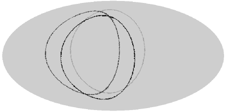
Figure 2: The Mollweide projection of $3$ intersecting circles. For clarity, the scan angle between the spin axis and the main beam axis is set to $60^{\circ}$ for this figure.

One of us Delabrouille (1998) has proposed to remove low frequency drifts for unpolarized data in the framework of the Planck mission by requiring that all measurements of a single point, from all the circles intersecting that point, share a common sky temperature signal. The problem is more complicated in the case of polarized measurements since the orientation of a polarimeter with respect to the sky depends on the scanning circle. Thus, a given polarimeter crossing a given point in the sky along two different circles will not measure the same signal, as illustrated in Fig. 3.

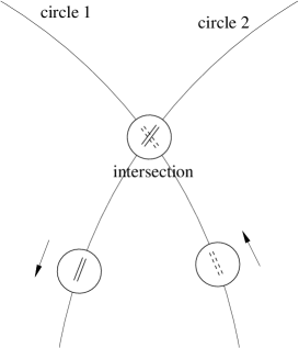
Figure 3: The orientation of polarimeters at an intersection point. This point is seen by two different circles corresponding to two different orientations of the polarimeters in the focal plane. For clarity, we have just represented one polarimeter.

The rest of the paper is organized as follows: in Sect. 2, we explain how we model the noise and how low frequency drifts transform into offsets when considering the circles instead of individual scans. In Sect. 3, we explain how polarization is measured. The details of the algorithm for removing low-frequency drifts are given in Sect. 4. We present the results of our simulations in Sect. 5 and give our conclusions in Sect. 6.

2 Averaging noise to offsets on circles

As shown in Fig. 1, the typical noise spectrum expected for the Planck High Frequency Instrument (HFI) features a drastic increase of noise power at low frequencies ${f\leq 0.01\leavevmode\nobreak\ \mathrm{Hz}}$. We model this noise spectrum as:

$$\!\!\!\!\!\!\!\!\!S(f)=\sigma^{2}\times\left(1+\sum_{i}\left(\frac{f_{i}}{f}\right)^{\alpha_{i}}\right).$$ (1)

The knee frequency ${f_{\mathrm{knee}}}$ is defined as the frequency at which the power spectrum due to low frequency contributions equals that of the white noise. The noise behaves as pure white noise with variance ${\sigma^{2}}$ at high frequencies. The spectral index of each component of the low-frequency noise, ${\alpha_{i}}$, is typically between 1 and 2, depending on the physical process generating the noise.

The Fourier spectrum of the noise on the circle obtained by combining $N$ consecutive scans depends on the exact method used. The simplest method, setting the circle equal to the average of all its scans, efficiently filters out all frequencies save the harmonics of the spinning frequency Delabrouille et al. (1998b). Since the noise power mainly resides at low frequencies (see Fig. 1), the averaging transforms – to first order – low frequency drifts into constant offsets different for each circle and for each polarimeter. This is illustrated in the comparison between Figs. 4 and 5. More sophisticated methods for recombining the data streams into circles can be used, as $\chi^{2}$ minimization, Wiener filtering, or any map-making method projecting about ${6\times 10^{5}}$ samples onto a circle of about ${5\times 10^{3}}$ points. For simplicity, we will work in the following with the circles obtained by simple averaging of all its consecutive scans.

Figure 4: Typical $1/f^{2}$ low frequency noise stream. Here, ${f_{\rm knee}=f_{\rm spin}=0.016}$ Hz, ${\alpha=2}$ and ${\sigma=21\leavevmode\nobreak\ \mu\mathrm{K}}$ (see Eq. 1). This noise stream corresponds to 180 scans or 3 circles (60 scans per circle) or a duration of 3 hours.

Figure 5: The residual noise on the 3 circles after averaging. To first approximation, low frequency drifts are transformed into offsets, different for each circle and each polarimeter. Note the expanded scale on the $y$-axis as compared to that of Fig. 4.

We thus model the effect of low frequency drifts as a constant offset for each polarimeter and each circle. This approximation is excellent for ${f_{\mathrm{knee}}\leq f_{\mathrm{spin}}}$. The remaining white noise of the $h$ polarimeters is described by one constant ${h\times h}$ matrix.

3 The measurement of sky polarization

3.1 Observational method

The measurement with one polarimeter of the linear polarization of a wave coming from a direction $\boldsymbol{\hat{n}}$ on the sky, requires at least three measurements with different polarimeter orientations. Since the Stokes parameters $Q$ and $U$ are not invariant under rotations, we define them at each point $\boldsymbol{\hat{n}}$ with respect to a reference frame of tangential vectors ${(\hat{e}_{\lambda},\hat{e}_{\beta})}$. The output signal given by a polarimeter looking at point $\boldsymbol{\hat{n}}$ is:

$$\!\!\!\!\!\!\!\!\!M_{polar}=\frac{1}{2}(I+Q\cos 2\Psi+U\sin 2\Psi)$$ (2)

where $\Psi$ is the angle between the polarimeter and $\hat{e}_{\lambda}$. In the following, we choose the longitude-latitude reference frame as the fixed reference frame on the sky (see Fig. 6).

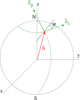
Figure 6: The reference frame used to define the Stokes parameters and angular position $\Psi$ of a polarimeter. $\Psi$ lies in the plane ${(\hat{e}_{\lambda},\hat{e}_{\beta})}$.

3.2 Destriping method

The destriping method consists in using redundancies at the intersections between circle pairs to estimate, for each circle $i$ and each polarimeter $p$, the offsets $O_{i}^{p}$ on polarimeter measurements. For each circle intersection, we require that all three Stokes parameters in a fixed reference frame in that direction of the sky, as measured on each of the intersecting circles, be the same. A $\chi^{2}$ minimization leads to a linear system whose solution gives the offsets. By subtracting these offsets, we can recover the Stokes parameters corrected for low-frequency noise.

3.3 Formalism

We consider a mission involving $n$ circles. The set of all circles that intercept circle $i$ is denoted by $\mathcal{I}(i)$ and contains $N_{\mathcal{I}(i)}$ circles. For any pair of circles $i$ and $j$, we denote the two points where these two circles intersect (if any) by ${\{i,j,\delta\}}$. In this notation $i$ is the circle currently scanned, $j$ the intersecting circle in set $\mathcal{I}(i)$, and $\delta$ indexes the two intersections ($\delta=1(-1)$ indexes the first (second) point encountered from the northernmost point on the circle) so that the points ${\{j,i,-\delta\}}$ and ${\{i,j,\delta\}}$ on the sky are identical.

The Stokes parameters at point $\{i,j,\delta\}$, with respect to a fixed global reference system, are denoted by a $3-$vector $\boldsymbol{S}_{i,j,\delta}$, with

$$\!\!\!\!\!\!\!\!\!\boldsymbol{S}_{i,j,\delta}=\boldsymbol{S}_{j,i,-\delta}=\left(\begin{array}[]{c}I\\ Q\\ U\end{array}\right)\left(\boldsymbol{\hat{n}}\equiv\{i,j,\delta\}\right).$$ (3)

At intersection $\{i,j,\delta\}$, the set of measurements by $h$ polarimeters travelling along the scanning circle $i$ is a $h-$vector denoted by $\boldsymbol{M}_{i,j,\delta}$, and is related to the Stokes parameters at this point by (see Eq. 2):

$$\!\!\!\!\!\!\!\!\!\boldsymbol{M}_{i,j,\delta}=\boldsymbol{\mathcal{A}}_{i,j,\delta}\boldsymbol{S}_{i,j,\delta}$$ (4)

where $\boldsymbol{\mathcal{A}}_{i,j,\delta}$ is the $h\times 3$ matrix:

$$\!\!\!\!\!\!\!\!\!\boldsymbol{\mathcal{A}}_{i,j,\delta}=\frac{1}{2}\left(\begin{array}[]{ccc}1&\cos 2\Psi_{1}(i,j,\delta)&\sin 2\Psi_{1}(i,j,\delta)\\ \vdots&\vdots&\vdots\\ 1&\cos 2\Psi_{p}(i,j,\delta)&\sin 2\Psi_{p}(i,j,\delta)\\ \vdots&\vdots&\vdots\\ 1&\cos 2\Psi_{h}(i,j,\delta)&\sin 2\Psi_{h}(i,j,\delta)\\ \end{array}\right).$$

$\Psi_{p}(i,j,\delta)\in[0,\pi]$ is the angle between the orientation of polarimeter $p$ and the reference axis in the fixed global reference frame (see Fig. 6). The matrix $\boldsymbol{\mathcal{A}}_{i,j,\delta}$ can be factorised as

$$\!\!\!\!\!\!\!\!\!\boldsymbol{\mathcal{A}}_{i,j,\delta}=\boldsymbol{\mathcal{A}}\boldsymbol{R}_{i,j,\delta}.$$ (5)

The constant $h\times 3$ matrix $\boldsymbol{\mathcal{A}}$ characterizes the geometrical setup of the $h$ polarimeters in the focal reference frame:

$$\!\!\!\!\!\!\!\!\!\boldsymbol{\mathcal{A}}=\frac{1}{2}\left(\begin{array}[]{ccc}1&1&0\\ \vdots&\vdots&\vdots\\ 1&\cos 2\Delta_{p}&\sin 2\Delta_{p}\\ \vdots&\vdots&\vdots\\ 1&\cos 2\Delta_{h}&\sin 2\Delta_{h}\\ \end{array}\right)$$ (6)

where $\Delta_{p}$ is the angle between the orientations of polarimeters $p$ and $1$, so we have $\Psi_{p}=\Psi_{1}+\Delta_{p}$ and $\Delta_{1}=0$. The rotation matrix $\boldsymbol{R}_{i,j,\delta}$ brings the focal plane to its position at intersection $\{i,j,\delta\}$ when scanning along circle $i$:

$$\!\!\!\!\!\!\!\!\!\boldsymbol{R}_{i,j,\delta}=\left(\begin{array}[]{ccc}1&0&0\\ 0&\cos 2\Psi_{1}(i,j,\delta)&\sin 2\Psi_{1}(i,j,\delta)\\ 0&-\sin 2\Psi_{1}(i,j,\delta)&\cos 2\Psi_{1}(i,j,\delta)\end{array}\right).$$ (7)

4 The algorithm

4.1 The general case

To extract the offsets from the measurements, we use a $\chi^{2}$ minimization. This $\chi^{2}$ relates the measurements $\boldsymbol{M}_{i,j,\delta}$ to the offsets $\boldsymbol{O}_{i}$ and the Stokes parameters $\boldsymbol{S}_{i,j,\delta}$, using the redundancy condition (3). In order to take into account the two contributions of the noise (see Sect. 2) and of the Stokes parameters (see Eq. 4), we model the measurement as:

$$\!\!\!\!\!\!\!\!\!\boldsymbol{M}_{i,j,\delta}=\boldsymbol{\mathcal{A}}\,\boldsymbol{R}_{i,j,\delta}\,\boldsymbol{S}_{i,j,\delta}\,+\boldsymbol{O}_{i}\,+\mathrm{white\leavevmode\nobreak\ noise}.$$ (8)

so that we write

$$\!\!\!\!\!\!\!\!\!\chi^{2}=\sum_{i,j\in{\mathcal{I}(i)},\delta=\pm 1}\,\left(\boldsymbol{M}_{i,j,\delta}-\boldsymbol{O}_{i}-\boldsymbol{\mathcal{A}}\,\boldsymbol{R}_{i,j,\delta}\,\boldsymbol{S}_{i,j,\delta}\right)^{T}\times\\ {\boldsymbol{N}_{i}}^{-1}\left(\boldsymbol{M}_{i,j,\delta}-\boldsymbol{O}_{i}-\boldsymbol{\mathcal{A}}\,\boldsymbol{R}_{i,j,\delta}\,\boldsymbol{S}_{i,j,\delta}\right).$$ (9)

where ${\boldsymbol{N}_{i}}$ is the $h\times h$ matrix of noise correlation between the $h$ polarimeters.

Minimization with respect to $\boldsymbol{O}_{i}$ and $\boldsymbol{S}_{i,j,\delta}$ yields the following equations:

$$\!\!\!\!\!\!\!\!\!{\boldsymbol{N}_{i}}^{-1}\sum_{j\in\mathcal{I}(i),\delta=\pm 1}\left(\boldsymbol{M}_{i,j,\delta}-\boldsymbol{O}_{i}-\boldsymbol{\mathcal{A}}\,\boldsymbol{R}_{i,j,\delta}\,\boldsymbol{S}_{i,j,\delta}\right)=0,\!\!\!\!\!\!\!\!\!$$ (10)

and

$$\!\!\!\!\!\!\!\!\!\boldsymbol{R}_{i,j,\delta}^{-1}\,\boldsymbol{\mathcal{A}}^{T}\,{\boldsymbol{N}_{i}}^{-1}\left(\boldsymbol{M}_{i,j,\delta}-\boldsymbol{O}_{i}-\boldsymbol{\mathcal{A}}\,\boldsymbol{R}_{i,j,\delta}\,\boldsymbol{S}_{i,j,\delta}\right)+$$

$$\!\!\!\!\!\!\!\!\!\boldsymbol{R}_{j,i,-\delta}^{-1}\boldsymbol{\mathcal{A}}^{T}{\boldsymbol{N}_{j}}^{-1}\left(\boldsymbol{M}_{j,i,-\delta}-\boldsymbol{O}_{j}-\boldsymbol{\mathcal{A}}\,\boldsymbol{R}_{j,i,-\delta}\,\boldsymbol{S}_{i,j,\delta}\right)=0.$$ (11)

We can work with a reduced set of transformed measurements and offsets which can be viewed as the Stokes parameters in the focal reference frame and the associated offsets which are the $3$ dimensional vectors:

$$\!\!\!\!\!\!\!\!\!\mathscr{S}_{i,j,\delta}={\boldsymbol{X}_{i}}^{-1}\,\boldsymbol{\mathcal{A}}^{T}\,{\boldsymbol{N}_{i}}^{-1}\boldsymbol{M}_{i,j,\delta}\mathrm{\leavevmode\nobreak\ \leavevmode\nobreak\ and\leavevmode\nobreak\ }$$

$$\!\!\!\!\!\!\!\!\!\boldsymbol{\Delta}_{i}={\boldsymbol{X}_{i}}^{-1}\,\boldsymbol{\mathcal{A}}^{T}\,{\boldsymbol{N}_{i}}^{-1}\boldsymbol{O}_{i},$$ (12)

$$\!\!\!\!\!\!\!\!\!\mbox{where }\boldsymbol{X}_{i}=\boldsymbol{\mathcal{A}}^{T}\,{\boldsymbol{N}_{i}}^{-1}\,\boldsymbol{\mathcal{A}}.$$

Eqs. (10) and (11) then simplify to:

$$\!\!\!\!\!\!\!\!\!\sum_{j\in\mathcal{I}(i),\,\delta=\pm 1}\left(\mathscr{S}_{i,j,\delta}-\boldsymbol{\Delta}_{i}-\boldsymbol{R}_{i,j,\delta}\,\boldsymbol{S}_{i,j,\delta}\right)=0,\!\!\!\!\!\!\!\!\!$$ (13)

and

$$\!\!\!\!\!\!\!\!\!\boldsymbol{R}_{i,j,\delta}^{-1}\,\boldsymbol{X}_{i}\,\left(\mathscr{S}_{i,j,\delta}-\boldsymbol{\Delta}_{i}-\boldsymbol{R}_{i,j,\delta}\,\boldsymbol{S}_{i,j,\delta}\right)+$$

$$\!\!\!\!\!\!\!\!\!\boldsymbol{R}_{j,i,-\delta}^{-1}\,\boldsymbol{X}_{j}\ \left(\mathscr{S}_{j,i,-\delta}-\boldsymbol{\Delta}_{j}-\boldsymbol{R}_{j,i,-\delta}\,\boldsymbol{S}_{i,j,\delta}\right)=0.$$ (14)

$\boldsymbol{R}_{i,j,\delta}\,\boldsymbol{S}_{i,j,\delta}$ in Eq. (14) can be solved for and the result inserted in Eq. (13). After a few algebraic manipulations, one gets the following linear system for the offsets $\boldsymbol{\Delta}_{i}$ as functions of the data $\mathscr{S}_{i,j,\delta}$:

$$\!\!\!\!\!\!\!\!\!\sum_{j\in\mathcal{I}(i),\delta=\pm 1}\left[\bbbone+\widetilde{\boldsymbol{R}}(i,j,\delta)\,{\boldsymbol{X}_{j}}^{-1}\,\widetilde{\boldsymbol{R}}(i,j,\delta)^{-1}\,\boldsymbol{X}_{i}\right]^{-1}\times\\ \!\!\!\!\!\!\!\!\!\!\!\!\!\!\!\!\!\!\left[\boldsymbol{\Delta}_{i}-\widetilde{\boldsymbol{R}}(i,j,\delta)\,\boldsymbol{\Delta}_{j}-\mathscr{S}_{i,j,\delta}+\widetilde{\boldsymbol{R}}(i,j,\delta)\,\mathscr{S}_{j,i,-\delta}\right]=0,$$ (15)

where the rotation

$$\!\!\!\!\!\!\!\!\!\widetilde{\boldsymbol{R}}(i,j,\delta)=\boldsymbol{R}_{i,j,\delta}\,{\boldsymbol{R}^{-1}_{j,i,-\delta}}$$ (16)

brings the focal reference frame from its position along scan $j$ at intersection $\{i,j,\delta\}$ to its position along scan $i$ at the same intersection (remember that $\{i,j,\delta\}=\{j,i,-\delta\}$). Note that $\widetilde{\boldsymbol{R}}(i,j,\delta)=\widetilde{\boldsymbol{R}}(j,i,-\delta)^{-1}$. In this linear system, we need to know the measurements of the polarimeters at the points $\{i,j,\delta\}$ and $\{j,i,-\delta\}$. These two points on circles $i$ and $j$ respectively will unlikely correspond to a sample along these circles. So we have linearly interpolated the value of the intersection points from the values measured at sampled points. For a fixed circle $i$, this is a $3\times N_{\mathcal{I}(i)}$ linear system. In Eq. (15), $i$ runs from $1$ to $n$, therefore the total matrix to be inverted has dimension $3n\times 3n$. However, because the rotation matrices are in fact two dimensional (see Eq. 7), the intensity components $\Delta_{i}^{I}$ of the offsets only enter Eq. (15) through their differences $\Delta_{i}^{I}-\Delta_{j}^{I}$ so that the linear system is not invertible: the rank of the system is $3n-1$. In order to compute the offsets, we can fix the intensity offset on one particular scanning circle or add the additionnal constraint that the length of the solution vector is minimized.

Once the offsets $\boldsymbol{\Delta}_{i}$ are known, the Stokes parameters in the global reference frame $\left(\hat{e}_{\lambda},\hat{e}_{\beta}\right)$ at a generic sampling $k$ of the circle $i$, labeled by $\{i,k\}$ are estimated as

$$\!\!\!\!\!\!\!\!\!\boldsymbol{S}_{i,k}=\boldsymbol{R}_{i,k}^{-1}\left(\mathscr{S}_{i,k}-\boldsymbol{\Delta}_{i}\right),$$ (17)

where $\boldsymbol{R}_{i,k}$ is the rotation matrix which transforms the focal frame Stokes parameters into those of the global reference frame.

The quantities $\mathscr{S}_{i,k}$ are the Stokes parameters measured in the focal frame of reference at this point and are simply given in terms of the measurements $\boldsymbol{M}_{i,k}$ (see Eq. 12) by:

$$\!\!\!\!\!\!\!\!\!\mathscr{S}_{i,k}={\boldsymbol{X}_{i}}^{-1}\,\boldsymbol{\mathcal{A}}^{T}\,{\boldsymbol{N}_{i}}^{-1}\boldsymbol{M}_{i,k}.$$ (18)

The matrix

$$\!\!\!\!\!\!\!\!\!\boldsymbol{N}^{\rm{Stokes}}_{i}=\left(\boldsymbol{\mathcal{A}}^{T}\,\boldsymbol{N}_{i}^{-1}\,\boldsymbol{\mathcal{A}}\right)^{-1}$$ (19)

is the variance matrix of the Stokes parameters on circle $i$. Note that this algorithm is totally independent of the pixelization chosen which only enters when reprojecting the Stokes parameters on the sphere.

4.2 Uncorrelated polarimeters, with identical noise

When the polarimeters are uncorrelated with identical noise, the variance matrix reduces to $\boldsymbol{N}_{i}=\bbbone/{\sigma_{i}}^{2}$ and the matrices $\boldsymbol{X}_{i}$ can all be written as

$$\!\!\!\!\!\!\!\!\!\boldsymbol{X}_{i}=\frac{1}{{\sigma_{i}}^{2}}\,\boldsymbol{X}\mbox{ with }\boldsymbol{X}=\boldsymbol{\mathcal{A}}^{T}\boldsymbol{\mathcal{A}}$$

Case of “Optimized Configurations”

We have shown Couchot et al. (1999) that the polarimeters can be arranged in “Optimized Configurations”, where the $h$ polarimeters are separated by angles of $\pi/h$. If the noise level of each of the $h$ polarimeters is the same and if there are no correlation between detector noise, then the errors of the Stokes parameters are also decorrelated and the matrix $\boldsymbol{X}$ has the simple form:

$$\!\!\!\!\!\!\!\!\!\boldsymbol{X}=\frac{n}{8}\left(\begin{array}[]{ccc}2&0&0\\ 0&1&0\\ 0&0&1\end{array}\right).$$ (20)

Because this matrix commutes with all rotation matrices $\widetilde{\boldsymbol{R}}(i,j,\delta)$, Eq. (15) simplifies further to

$$\!\!\!\!\!\!\frac{N_{\mathcal{I}(i)}}{\sigma_{\mathcal{I}(i)}^{2}}\boldsymbol{\Delta}_{i}-\sum_{{m\in{\mathcal{I}(i)}}}\frac{1}{\sigma_{i}^{2}+\sigma_{j}^{2}}\left(\widetilde{\boldsymbol{R}}(i,j,1)+\widetilde{\boldsymbol{R}}(i,j,-1)\right)\boldsymbol{\Delta}_{j}\\ \!\!\!\!\!\!\!\!\!=\sum_{j\in{\mathcal{I}(i)},\delta=\pm 1}\frac{1}{\sigma_{i}^{2}+\sigma_{j}^{2}}\left(\mathscr{S}_{i,j,\delta}-\widetilde{\boldsymbol{R}}(i,j,\delta)\,\mathscr{S}_{j,i,-\delta}\right),$$ (21)

where the sum over $\delta$ is explicit on the left side of the equation and we have defined an average error $\sigma_{\mathcal{I}(i)}$ along circle $i$ by

$$\!\!\!\!\!\!\!\!\!\frac{N_{\mathcal{I}(i)}}{\sigma_{\mathcal{I}(i)}^{2}}=\sum_{j\in{\mathcal{I}(i)}}\frac{2}{\sigma_{i}^{2}+\sigma_{j}^{2}},$$

and where the rotation matrix $\widetilde{\boldsymbol{R}}(i,j,\delta)$ is defined by Eq. (16). Rotations $\widetilde{\boldsymbol{R}}(i,j,\delta)$ and $\widetilde{\boldsymbol{R}}(i,j,-\delta)=\widetilde{\boldsymbol{R}}(j,i,\delta)^{-1}$ correspond to the two intersections between circles $i$ and $j$. Eq. (21) can be simplified further. We can separate the $\boldsymbol{\Delta}_{i}$ and the $\mathscr{S}_{i,j,\delta}$ into scalar components related to the intensity: $\Delta^{I}_{i},\ \mathscr{S}^{I}_{i,j,\delta}$ and 2-vectors components related to the polarization: $\boldsymbol{\Delta}^{P}_{i},\ \mathscr{S}^{P}_{i,j,\delta}$. We obtain then two separate equations, one for the intensity offsets $\Delta^{I}_{i}$, which is exactly the same as in the unpolarized case (see A):

$$\!\!\!\!\!\!\sum_{j\in{\mathcal{I}(i)}}\frac{2}{\sigma_{i}^{2}+\sigma_{j}^{2}}\,\left(\Delta^{I}_{i}-\Delta^{I}_{j}\right)=\\ \!\!\!\!\!\!\!\!\!\qquad\qquad\sum_{j\in{\mathcal{I}(i)},\delta=\pm 1}\frac{1}{\sigma_{i}^{2}+\sigma_{j}^{2}}\left(\mathscr{S}^{I}_{i,j,\delta}-\mathscr{S}^{I}_{j,i,-\delta}\right),$$ (22)

and one for the polarization offsets $\boldsymbol{\Delta}^{P}_{i}$:

$$\!\!\!\!\!\!\frac{N_{\mathcal{I}(i)}}{\sigma_{\mathcal{I}(i)}^{2}}\,\boldsymbol{\Delta}^{P}_{i}-\sum_{j\in{\mathcal{I}(i)}}\frac{2}{\sigma_{i}^{2}+\sigma_{j}^{2}}\,\cos\left(2\Psi_{ij}\right)\,\boldsymbol{\Delta}^{P}_{j}=\\ \!\!\!\!\!\!\!\!\!\sum_{j\in{\mathcal{I}(i)},\delta=\pm 1}\frac{1}{\sigma_{i}^{2}+\sigma_{j}^{2}}\left(\mathscr{S}^{P}_{i,j,\delta}-\boldsymbol{\mathcal{R}}(i,j,\delta)\,\mathscr{S}^{P}_{j,i,-\delta}\right),$$ (23)

where $\Psi_{ij}=\Psi_{1}(i,j,\delta)-\Psi_{1}(j,i,-\delta)$ is the angle of the rotation that brings the focal reference frame along scan $j$ on the focal reference frame along scan $i$ at intersection $\{i,j,\delta\}$. The two dimensional matrix $\boldsymbol{\mathcal{R}}(i,j,\delta)$ is the rotation sub-matrix contained in $\widetilde{\boldsymbol{R}}(i,j,\delta)$ (see Eq. 16). Note that all mixing between polarization components have disappeared from the left side of Eq. (23)). Therefore we are left with two different $n\times n$ matrices to invert in order to solve for the offsets $\boldsymbol{\Delta}_{i}$, instead of one $3n\times 3n$ matrix.

As in Eq. (15), the linear system in Eq. (22) involves differences between the offsets $\Delta_{i}^{I}$, the matrix is not invertible, and we find the solution in the same way as in the general case. On the other hand, for the polarized offsets $\Delta_{i}^{P}$, the underlying matrix of Eq. (23) is regular as expected.

5 Simulations and test of the algorithm

5.1 Methods

We now discuss how we test the method using numerical simulations. For each simulated mission, we produce several maps. The first, which we use as the standard “reference” of comparison, is a projected map of a mission with only white noise, ${f_{\mathrm{knee}}=0}$. The remaining maps include $1/f$ plus white noise streams with ${f_{\mathrm{knee}}=\eta f_{\mathrm{spin}}}$, ${\eta\in\{1,2,5,10\}}$. The first of these is an “untreated” image which is projected with no attempt to remove striping affects. In the second “zero-averaged” map, we attempt a crude destriping by subtracting its average to each circle. The final “destriped” map is constructed using the algorithm in this paper. We subtract the input maps ($I$, $Q$ and $U$) from the final maps in order to get maps of noise residuals. Note that in case of a zero signal sky, setting the average of each circle to zero is better than destriping by nature because the offsets are only due to the noise. With a real sky, both signal and noise contribute to the average so that zeroing circle not only removes the noise but also the signal. Giard et al Giard et al. (1999) have attempted to refine their method by fitting templates of the dipole and of the galaxy before subtracting a baseline from each circle. They concluded that an additional destriping (they used the algorithm of Delabrouille Delabrouille (1998)) is needed.

5.2 Simulated missions

In order to test its efficiency, the destriping algorithm has been applied to raw data streams generated from simulated observations using various circular scanning strategies representative of a satellite mission as Planck, different “Optimized Configurations”, and various noise parameters. The resulting maps were then compared with input and untreated maps to test the quality of the destriping.

The input temperature ($I$) maps are the sum of galaxy, dipole, and a randomly generated standard CDM anisotropy map (we used HEALPIX and CMBfast). Similarly, the polarization maps $Q$ and $U$ are the sum of the galaxy and CMB polarizations. The CMB polarization maps are randomly generated assuming a standard CDM scenario. For the galactic polarization maps, we constructed a random, continuous and correlated vector field defined on the 2-sphere with a correlation length of $5^{\circ}$ and a maximum polarization rate of ${20\%}$ ($100\%$ gave similar results). Given the temperature map of the sky (not including CMB contribution), we can thus construct two polarization maps for $Q$ and $U$.

5.3 Results

We first consider the case of destriping pure white noise and check that the destriping algorithm does not introduce spurious structure. Once this is verified, we apply the destriping algorithm to low frequency noise. We find that the quality of the destriping is significantly dependent on $\eta$ only. To demonstrate visually the quality of the destriping, we produce projected sky maps with the input galaxy, dipole and CMB signal subtracted.

For temperature maps, we can compare Figs. 7,8, and 9. The eye is not able to see any differences between the white noise map and the noise residual on the destriped map. We will see in the following how to quantify the presence of structures. For the “zero-averaged circles” map, the level of the structure is very high and make it impossible to compute the power spectrum of the CMB (see Fig. 13).

For the $Q$ Stokes parameter, Fig. 11 shows the destriped map for $\eta=1$. Fig. 12 shows a map where the offsets are calculated as the average of each circle. The maps for $U$ are very similar. As for the $I$ maps, the destriped map is very similar to the white noise map. There exist some residual structure on the “zero-averaged circles” map. To assess quantitatively the efficiency of the destriping algorithm, we have first studied the power spectra $C_{\ell}^{T}$, $C_{\ell}^{E}$, $C_{\ell}^{B}$, $C_{\ell}^{TE}$ and $C_{\ell}^{TB}$ calculated from the $I$, $Q$ and $U$ maps Zaldarriaga and Seljak (1997); Kamionkowski et al. (1997).

Figure 7: The Mollweide projection of the residuals of the ${I-\mathrm{Stokes}}$ parameter for a white noise mission. The scale is in Kelvins. The parameters of the simulation leading to this map are described in B.

Figure 8: The Mollweide projection of the residuals of the ${I-\mathrm{Stokes}}$ parameter after destriping of $1/f$ noise plus white noise with $\eta=1$

Figure 9: The Mollweide projection of the residuals of the ${I-\mathrm{Stokes}}$ parameter after zeroing the average of the circles, for $1/f$ noise plus white noise with $\eta=1$.

Figure 10: The Mollweide projection of the residuals of the ${Q-\mathrm{Stokes}}$ parameter for a white noise mission.

Figure 11: The Mollweide projection of the residuals of the ${Q-\mathrm{Stokes}}$ parameter after destriping of $1/f$ noise plus white noise with $\eta=1$

Figure 12: The Mollweide projection of the residuals of the ${Q-\mathrm{Stokes}}$ parameter after zeroing the average of the circles, for $1/f$ noise plus white noise with $\eta=1$. Although the remaining structures seem small, they are responsible for the excess of power in ${C_{\ell}^{E}}$, see Fig. 16.

The reference sensitivity of our simulated mission is evaluated by computing the average spectra of 1000 maps of reprojected mission white noise. This reference sensitivity falls, within sample variance, between the two dotted lines represented in Figs. 13, 14, 15 and 16 and below the dotted line in Figs. 17 and 18. Figs. 13 and 14 show the spectra ${C_{\ell}^{T}}$ corresponding to ${f_{\mathrm{knee}}/f_{\mathrm{spin}}=1\mathrm{\leavevmode\nobreak\ and\leavevmode\nobreak\ }5}$ respectively, for the $T$ field. Similarly, Figs. 15 and 16 are the spectra ${C_{\ell}^{E}}$. The $B$ field is not represented because it is very similar to $E$. Figs. 17 and 18 represent the correlation between $E$ and $T$: $C_{\ell}^{ET}$. For ${f_{\mathrm{knee}}/f_{\mathrm{spin}}=1}$, we see that we are able to remove very efficiently low frequency drifts in the noise stream: the destriped spectra obtained are compatible with the white spectrum (within sample variance). Similar quality destriping is achieved for any superposition of $1/f$, $1/f^{2}$ and white noise, provided that the knee frequency is lower than or equal to the spin frequency. In the case of ${f_{\mathrm{knee}}/f_{\mathrm{spin}}=5}$, the method as implemented here leaves some striping noise on the maps at low values of $\ell$. Modeling the noise as an offset is no longer adequate and a better model of the averaged low-frequency noise is required (superposition of sine and cosine functions for instance), or a more sophisticated method for constructing one circle from 60 scans. We again note that the value of the ratio ${f_{\mathrm{knee}}/f_{\mathrm{spin}}}$ for both Planck HFI and LFI is likely to be very close to unity (in Fig. 1, ${f^{\mathrm{measured}}_{\mathrm{knee}}\sim 0.014}$ Hz and ${f_{\mathrm{spin}}=0.016}$ Hz).

To quantify the presence of stripes in the maps of residuals, we can compute the value of the “striping” estimator ${\mathrm{rms}(a^{T,E,B}_{\ell\ell})/\mathrm{rms}(a^{T,E,B}_{\ell 0})}$, because stripes tend to appear as structure grossly parallel to the iso-longitude circles. In the case of pure white noise with a uniform sky coverage, this value is 1. Here, because of the scanning strategy, the sky coverage is not uniform and the value of this estimator is greater than 1, showing that it is not specific of the striping. In order to get rid of the effect of non-uniform sky coverage, we express the estimator ${\mathrm{rms}(a^{T,E,B}_{\ell\ell})/\mathrm{rms}(a^{T,E,B}_{\ell 0})}$ in units of ${\mathrm{rms}(a^{T,E,B}_{\ell\ell})/\mathrm{rms}(a^{T,E,B}_{\ell 0})}$ for the white noise. This new estimator is specific to the striping. The results in Table 1 show the improvement achieved by the destriping algorithm although the result is still not perfect.

Table 1: Values of ${\mathrm{rms}(a^{T,E,B}_{\ell\ell})/\mathrm{rms}(a^{T,E,B}_{\ell 0})}$ as a function of ${\eta={f_{\mathrm{knee}}/f_{\mathrm{spin}}}}$ in units of ${\mathrm{rms}(a^{T,E,B}_{\ell\ell}(\mathrm{WN}))/\mathrm{rms}(a^{T,E,B}_{\ell 0}(\mathrm{WN}))}$ We have checked that the systematic difference between the zero-averaged $E$ and $B$ fields is randomly in favor of $E$ and $B$ depending on the particular sky simulation.

Method	${f_{\mathrm{knee}}/f_{\mathrm{spin}}}$	$T$	$E$	$B$
white noise	0	1	1	1
destriped	0.5	1.19	1.05	1.03
zero-averaged	0.5	51.9	9.23	3.64
undestriped	0.5	6.98	7.04	15.2
destriped	1	1.24	1.12	1.19
zero-averaged	1	52.2	9.91	3.95
undestriped	1	10.7	10.9	7.51
destriped	2	1.26	1.32	1.23
zero-averaged	2	49.5	10.2	3.85
undestriped	2	6.41	9.97	8.18
destriped	5	1.35	1.39	1.38
zero-averaged	5	49.8	10.4	3.99
undestriped	5	11.3	8.24	12.4

Figure 13: Efficiency of destriping for the $T$ field with ${f_{\rm knee}/f_{\rm spin}=1}$. The sample variance associated to a pure white noise mission is plotted as the dotted lines. The “destriped spectrum” is very close to the white noise spectrum (within the limits due to the sample variance). The zero-averaged and the “not destriped” spectra are a couple of orders of magnitude above. The solid line represents a standard CDM temperature spectrum and the dashed line represents a CDM temperature spectrum with reionization.

Figure 14: Efficiency of destriping for the $T$ field with ${f_{\rm knee}/f_{\rm spin}=5}$. The modelling of low-frequency noise with an offset is no longer sufficient and the destriping leaves some power at low values of $\ell$. Nevertheless, it remains a very good way to significantly reduce the effect of low-frequency noise.

Figure 15: Efficiency of destriping for the $E$ field for ${f_{\rm knee}/f_{\rm spin}=1}$. The zero-averaged spectrum is not as bad as for $T$ but the residual striping we can see in Fig. 12 leads to some excess of power for low values of $\ell$ (up to $\ell\sim 100$). We do not see such effect in the destriped spectrum (and maps). The spectra for the $B$ fields are very similar. The solid line represents a standard CDM $E$ spectrum and the dashed line represents a CDM $E$ spectrum with reionization.

Figure 16: Same as Fig. 16 but for ${f_{\rm knee}/f_{\rm spin}=5}$. The spectra for the $B$ fields are very similar.

Figure 17: Same as Fig. 16 for the $ET$-correlation for ${f_{\rm knee}/f_{\rm spin}=1}$.

Figure 18: Same as Fig. 18 but for ${f_{\rm knee}/f_{\rm spin}=5}$.

6 Discussions and Conclusions

Comparison with other methods.

Although no other method has yet been developped specifically for destriping polarized data, many methods exist for destriping unpolarized CMB data, which could be adapted to polarized data as well.

We first comment on the classical method which consists in modelling the measurement as

$$m_{t}=A_{tp}T_{p}+n_{t}$$ (24)

where $A$ is the so-called ”pointing matrix”, $T$ a vector of temperatures in pixels of the sky, $m_{t}$ the data and $n_{t}$ the noise. The problem is solved by inversion, yielding an estimator of the signal:

$$\tilde{T_{p}}=[A^{t}N^{-1}A]^{-1}A^{t}N^{-1}\,m,$$ (25)

where $N=\langle nn^{t}\rangle$ is the noise correlation matrix and $A^{t}$ is the transposed matrix of $A$.

This method can be extended straightforwardly to polarized measurements, at the price of extending by a factor of $3\times h$ the size of the matrix $A_{tp}$, by 3 that of vector $T_{p}$ (replaced by $(I_{p},Q_{p},U_{p})$), and by $h$ that of the data stream (remember that $h$ is the number of polarimeters). The implementation of this formally simple solution may turn into a formidable problem when megapixel maps are to be produced. Numerical methods have been proposed by a variety of authors Wright (1996); Tegmark (1997), that use properties of the noise correlation matrix (symmetry, band-diagonality) and of the pointing matrix (sparseness). Such methods, however, rely critically on the assumption that the noise is a Gaussian, stationary random process, which has been a reasonable assumption for CMB mission as COBE where the largest part of the uncertainty comes from detector noise, but is probably not so for sensitive missions such as Planck. Our method requires only inverting a ${3n\times 3n}$ matrix where $n$ is the number of circles involved, and does not assume anything on the statistical properties of low frequency drifts. It just assumes a limit frequency (the knee frequency) above which the noise can be considered as a white Gaussian random process.

Another interesting method is the one that has been used by Ganga in the analysis of FIRS data Ganga (1994), which is itself adapted from a method developed originally by Cottingham Cottingham (1987). In that method, coefficients for splines fitting the low temperature drifts are obtained by minimising the dispersion of measurements on the pixels of the map. Such a method, very similar in spirit to ours, could be adapted to polarization. Splines are natural candidates to replace our offsets in refined implementations of our algorithm.

Here, we have assumed that the averaged noise can be modeled as circle offsets plus white noise (Eq. 8), i.e. that the noise between different measurements from the same bolometer is uncorrelated after removal of the offset. This allowed us to simplify the $\chi^{2}$ to that shown in Eq. (9). In reality, the circular offsets do not completely remove the low frequency noise and there does remain some correlation between the measurements. The amount of correlation is directly related to the value of ${f_{\mathrm{knee}}/f_{\mathrm{spin}}}$; the smaller ${f_{\mathrm{knee}}/f_{\mathrm{spin}}}$ the smaller the remaining correlation. Figs. 13-18 already contain the errors induced from the fact that we did not include these correlations in the covariance matrix, and thus demonstrate that the effect is small for ${f_{\mathrm{knee}}/f_{\mathrm{spin}}\sim 1}$.

Conclusion.

The destriping as implemented in this paper removes low frequency drifts up to the white noise level provided that ${f_{\mathrm{knee}}/f_{\mathrm{spin}}\leq 1}$. For larger ${f_{\mathrm{knee}}}$, the simple offset model for the averaged noise could be replaced with a more accurate higher-order model that destripes to better precision provided the scan strategy allows to do so, as discussed in Delabrouille et al Delabrouille et al. (1998a). We are currently working on improving our algorithm to account for these effects. However, despite the shortcomings of our model, it still appears to be robust for small ${f_{\mathrm{knee}}}$ and can serve as a first order analysis tool for real missions. In particular, our technique cannot only be used for the Planck HFI and LFI, but can also be adopted for other CMB missions with circular scanning strategies, such as COSMOSOMAS for instance Rebolo et al. (1999).

Appendix A Destriping of unpolarized data

We give here the formulæ for the simpler case of destriping temperature measurements with bolometers. The assumptions are the same as in the polarized case and we adopt the same notation for the common quantities. Instead of polarimeters, we have $h$ bolometers. Since the measurement is no longer dependent on the orientation of the bolometer, the model of the measurement is given by:

$$\!\!\!\!\!\!\!\!\!\boldsymbol{M}_{i,j,\delta}=\boldsymbol{O}_{i}+I_{i,j,\delta}\leavevmode\nobreak\ \boldsymbol{u}\mathrm{\leavevmode\nobreak\ \leavevmode\nobreak\ with\leavevmode\nobreak\ \leavevmode\nobreak\ }\boldsymbol{u}=\left(\begin{array}[]{c}1\\ \vdots\\ 1\end{array}\right)$$ (26)

where ${\boldsymbol{M}_{i,j,\delta}}$ is the $h-$vector made of measurements by the $h$ bolometers, ${\boldsymbol{O}_{i}}$ is an $h-$vector containing the offsets for the i’th circle and ${I_{i,j,\delta}}$ is the temperature in the direction of the intersection point labeled by $\{i,j,\delta\}$. $\boldsymbol{u}$ is an $h$-vector, corresponding to the $\boldsymbol{\mathcal{A}}$ matrix of the polarized case. The $\chi^{2}$ can be written as:

$$\!\!\!\!\!\!\!\chi^{2}=\sum_{i,j\in{\mathcal{I}(i)},\delta=\pm 1}\,\left(\boldsymbol{M}_{i,j,\delta}-\boldsymbol{O}_{i}-I_{i,j,\delta}\;\boldsymbol{u}\right)^{T}\times\\ {\boldsymbol{N}_{i}}^{-1}\left(\boldsymbol{M}_{i,j,\delta}-\boldsymbol{O}_{i}-I_{i,j,\delta}\;\boldsymbol{u}\right).$$ (27)

In this case, the physical quantity uniquely defined at an intersection point is the temperature of the sky at this point. The constraint used here for removing low-frequency noise is then:

$$\!\!\!\!\!\!\!\!\!I_{i,j,\delta}=I_{j,i,-\delta}.$$ (28)

Given this relation, the minimization of the $\chi^{2}$ with respect to $\boldsymbol{O}_{i}$ and $I_{i,j,\delta}$ leads to the linear system:

$$\!\!\!\!\!\!\sum_{j\in\mathcal{I}(i)}\frac{x_{j}}{x_{i}+x_{j}}\left(\Delta_{i}-\Delta_{j}\right)=\\ \frac{1}{2}\sum_{j\in\mathcal{I}(i),\delta=\pm 1}\frac{x_{j}}{x_{i}+x_{j}}\left(\mathscr{I}_{i,j,\delta}-\mathscr{I}_{j,i,-\delta}\right)$$ (29)

where

$$\!\!\!\!\!\!\!\!\!x_{i}=\boldsymbol{u^{T}}\,\boldsymbol{N}_{i}^{-1}\,\boldsymbol{u}$$ (30)

corresponds to the $\boldsymbol{X}_{i}$ matrix of the polarized case,

$$\!\!\!\!\!\!\!\!\!\mathscr{I}_{i,j,\delta}=\frac{1}{x_{i}}\,\boldsymbol{u^{T}}\,\boldsymbol{N}_{i}^{-1}\,\boldsymbol{M}_{i,j,\delta}$$ (31)

corresponds to the $\mathscr{S}_{i,j,\delta}$ local Stokes parameters of the polarized case and the scalar

$$\!\!\!\!\!\!\!\!\!\Delta_{i}=\frac{1}{x_{i}}\,\boldsymbol{u^{T}}\,\boldsymbol{N}_{i}^{-1}\,\boldsymbol{O}_{i}$$ (32)

corresponds to the 3-vector $\Delta_{i}$ of the polarized case.

Temperature offsets appear through their differences $\Delta_{i}-\Delta_{j}$ so this linear system is not invertible and we can use the same methods to invert the system than in the polarized case. The size of the matrix to invert is $n\times n$.
After evaluation of the offsets $\Delta_{i}$, one can recover the value of temperature for any sample $k$ along circle $i$:

$$\!\!\!\!\!\!\!\!\!I_{i,k}=\mathscr{I}_{i,k}-\Delta_{i}.$$ (33)

Appendix B Details of the simulations

The results presented in this paper correspond to the “Optimized Configuration” involving $3$ polarimeters and to an angular step of $18^{\prime}$: the angle between two consecutive samples along a circle is $18^{\prime}$ and there is one circle every $18^{\prime}$.

In this case, the number of circles is $n_{\mathrm{c}}=1200$ and the number of samples on each circle is $n_{\mathrm{s}}=1195$. The spin axis has a sinusoidal motion around the ecliptic plane with an amplitude of $8^{\circ}$ and with $8$ cycles during the mission. The aperture angle of the circles is $85^{\circ}$. The simulated noise has ${f_{\mathrm{knee}}=\eta f_{\mathrm{spin}}}$ with ${\eta=1\mathrm{\leavevmode\nobreak\ and\leavevmode\nobreak\ }5}$.

The white noise variance is calculated based on the expected sensitivity on $Q$ and $U$ ($3.7\leavevmode\nobreak\ \mu$K/K) of the (arbitrarily selected) 143 GHz polarized channel of the Planck mission.

All the maps (CMB, dipole, galaxy, simulation) are HEALPIX maps with 196 608 pixels of $27.48^{\prime}$. Only 12 pixels ($0.006\%$ of the map) are not seen by the mission: their values are set to the average of the map. The signal maps have been smoothed by a gaussian beam with a FWHM set to ${2.5\times 18^{\prime}}$.

We have run other simulations with “Optimized Configuration” involving $3$ or $4$ polarimeters, and with cycloidal, sinusoidal or anti-solar spin axis trajectories (see Bersanelli et al Bersanelli et al. (1996) and the Planck web page for additionnal information about proposed scanning strategies). The aperture angle of the circles have been taken in $[70^{\circ},75^{\circ},80^{\circ},85^{\circ},90^{\circ}]$. In all these cases, the results are similar for ${f_{\mathrm{knee}}/f_{\mathrm{spin}}\sim 1}$. For more pessimistic noise cases, the choice of the scanning strategy may have a strong impact on the quality of the final maps. A quantitative study of this point is deffered to a forthcoming publication.

References

- Bersanelli et al. (1996) Bersanelli, M. et al.: 1996, Report on the phase A study, Technical report, ESA, D/SCI(96)3
- Cottingham (1987) Cottingham, D.: 1987, Ph.D. thesis, Princeton University
- Couchot et al. (1999) Couchot, F., Delabrouille, J., Kaplan, J., and Revenu, B.: 1999, Astronomy & Astrophysics Supplement Series 135, 579
- Delabrouille (1998) Delabrouille, J.: 1998, Astronomy & Astrophysics Supplement Series 127, 555
- Delabrouille et al. (1998a) Delabrouille, J., Gispert, R., Puget, J.-L., and Lamarre, J.: 1998a, astro-ph/9810478
- Delabrouille et al. (1998b) Delabrouille, J., Górski, K. M., and Hivon, E.: 1998b, Mon. Not. R. Astron. Soc. 298, 445
- Ganga (1994) Ganga, K.: 1994, Ph.D. thesis, http://spider.ipac.caltech.edu/staff/kmg/
- Giard et al. (1999) Giard, M., Hivon, E., Nguyen, C., Gispert, R., Górski, K., and Lange, A.: 1999, astro-ph/9907208
- Kamionkowski (1998) Kamionkowski, M.: 1998, astro-ph/9803168
- Kamionkowski et al. (1997) Kamionkowski, M., Kosowsky, A., and Stebbins, A.: 1997, Phys. Rev. D 55, 7368
- Kinney (1998) Kinney, W.: 1998, astro-ph/9806259
- Prunet and Lazarian (1999) Prunet, S. and Lazarian, A.: 1999, astro-ph/9902314
- Rebolo et al. (1999) Rebolo, R., Gutiérrez, C., Watson, R., and Gallegos, J.: 1999, in Proceedings of the Workshop ”The CMB and the Planck Mission” held in Santander, to appear in Astrophysical Letters and Communications
- Seljak (1996) Seljak, U.: 1996, astro-ph/9608131
- Tegmark (1997) Tegmark, M.: 1997, Phys. Rev. D 56, 4514
- Wright (1996) Wright, E. L.: 1996, astro-ph/9612006
- Zaldarriaga (1998) Zaldarriaga, M.: 1998, Ph.D. thesis, astro-ph/9806122
- Zaldarriaga and Seljak (1997) Zaldarriaga, M. and Seljak, U.: 1997, Phys. Rev. D 55, 1830