On Planetary Companions to the MACHO-98-BLG-35 Microlens Star

Abstract

We present observations of microlensing event MACHO-98-BLG-35 which reached a peak magnification factor of almost 80. These observations by the Microlensing Planet Search (MPS) and the MOA Collaborations place strong constraints on the possible planetary system of the lens star and show intriguing evidence for a low mass planet with a mass fraction $4\times 10^{-5}\leq\epsilon\leq 2\times 10^{-4}$. A giant planet with $\epsilon=10^{-3}$ is excluded from 95% of the region between 0.4 and 2.5 $R_{E}$ from the lens star, where $R_{E}$ is the Einstein ring radius of the lens. This exclusion region is more extensive than the generic “lensing zone” which is $0.6-1.6R_{E}$. For smaller mass planets, we can exclude 57% of the “lensing zone” for $\epsilon=10^{-4}$ and 14% of the lensing zone for $\epsilon=10^{-5}$. The mass fraction $\epsilon=10^{-5}$ corresponds to an Earth mass planet for a lensing star of mass $\sim 0.3\rm{M_{\odot}}$. A number of similar events will provide statistically significant constraints on the prevalence of Earth mass planets. In order to put our limits in more familiar terms, we have compared our results to those expected for a Solar System clone averaging over possible lens system distances and orientations. We find that such a system is ruled out at the 90% confidence level. A copy of the Solar System with Jupiter replaced by a second Saturn mass planet can be ruled out at 70% confidence. Our low mass planetary signal (few Earth masses to Neptune mass) is significant at the $4.5\sigma$ confidence level. If this planetary interpretation is correct, the MACHO-98-BLG-35 lens system constitutes the first detection of a low mass planet orbiting an ordinary star without gas giant planets.  

(The MOA Collaboration)

1 Introduction

Planetary systems in the foreground of the Galactic bulge or inner Galactic disk form a class of gravitational lens systems that can be detected through photometric microlensing measurements. These are multiple lens systems although in most cases, the light curve is not easily distinguished from a single lens light curve. A planet perturbs the gravitational potential of its host star ever so slightly, and its effect may manifest itself as a brief variation of the would-be single lens microlensing light curve Mao & Paczynski (1991); Gould & Loeb (1992); Bolatto & Falco (1994). With sufficiently frequent and accurate observations, it is possible to detect planets with masses as small as that of the Earth Bennett & Rhie (1996) and measure the fractional mass $\epsilon$ and the (projected) distance of the planet $a$ from the host lens star. This complements other ground based extra-solar planet search techniques Marcy & Butler (1998) which have sensitivities that are not expected to extend much below the mass fraction of Saturn ($3\times 10^{-4}$).

Planned space based observatories, such as the Space Interferometry Mission (SIM) Allen, Peterson & Shao (1997) or the proposed Terrestrial Planet Finder (TPF) Beichman (1998), Darwin Penny et al. (1998), and Kepler Koch et al. (1998) satellites can not only detect planets as small as the Earth, but they can also study a number of their properties. However, the prevalence of low mass planets is not known, and the recent planetary discoveries via the radial-velocity technique Marcy & Butler (1998) suggest that our current understanding of planetary system formation is incomplete. Circumstellar disks of less than a Jupiter mass around young stellar objects have been found with multiwavelength observations Padgett et al. (1999). These could indicate the formation of planetary systems without massive planets, but it is also possible that massive planets have already formed in such systems. Thus, microlensing can provide valuable statistical information on the abundance of low mass planets that can be used to aid in the design of these future space missions Elachi et al. (1996).

The planetary signal in a gravitational microlensing event can be quite spectacular due to the singular behavior of the caustics, but the signal is always quite brief compared to the duration of the stellar lensing event. The small size of the caustic curves ($\approx\cal{O}(\sqrt{\epsilon})$) more or less determines the planetary signal timescale. The caustics of a planetary binary lens consist of the stellar caustic (very near the stellar lens) and planetary caustic(s), and the detection probability of the planet depends on the size and geometric distribution of the caustics which in turn depend on the fractional mass $\epsilon$ and the (projected) distance $a$ of the planet from the stellar lens. Theoretical estimations based upon a variety of “reasonable” detection criteria have shown that the detection probability of a planet with $\epsilon=10^{-3}$ is about 20% Gould & Loeb (1992); Wambsganss (1997); (Gaudi, Naber, & Sackett1998); Di Stefano & Scalzo (1999, 1999), and for Earth-mass planets orbiting an M-dwarf primary ($\epsilon\approx 10^{-5}$), it is only about 2% Bennett & Rhie (1996). Thus, microlensing planet search programs must generally observe a large number of microlensing events in order to detect planetary lensing events even if planets are ubiquitous.

For high magnification events with peak magnification $A_{\rm max}\hbox{ \hbox to0.0pt{\raise 1.82986pt\hbox{$>$}\hss}\lower 2.79857pt\hbox{$\sim$} }20$, the stellar caustic can cause planetary perturbations to the lightcurve, and the probability of detecting planets is very high Griest & Safizadeh (1998). For example, the detection probability for a giant planet in the “lensing zone” is close to $100\%$ for a microlensing event like MACHO-98-BLG-35 where the peak magnification was about 80. High magnification occurs when the impact distance is much smaller than the Einstein ring radius ($1\gg u_{\rm min}\simeq 1/A_{\rm max}$), so the source comes very close to the location of the stellar caustic. ($u_{\rm min}$ is the impact distance in units of the Einstein ring radius.) If we recall that a single lens (stellar lens only) has a point caustic at the position of the lens, the stellar caustic of a planetary binary lens can be considered as this point caustic extended to a finite size due to the gravitational perturbation of the planet. For a large range of planetary mass fractions and separations, the stellar caustic will be perturbed by the planet, and this will be visible near the lightcurve peak of a high magnification event, whose timing can be predicted fairly accurately. Thus, high magnification events offer the opportunity to detect a planet in a large range of locations in the vicinity of the lens star. High magnification events are relatively rare, with a probability $\sim u_{\rm min}$, but when they occur, they should be observed relentlessly.

Event MACHO-98-BLG-35 was the highest magnification microlensing event observed to date, and it was one of the first high magnification events that was closely monitored for evidence of planets near peak magnification (see also Gaudi et al. 1998). In this paper, we present a joint analysis of the MACHO-98-BLG-35 data from the Microlensing Planet Search (MPS) and MOA collaborations. This analysis yields evidence consistent with a planet in the mass range $4\times 10^{-5}\leq\epsilon\leq 2\times 10^{-4}$ which would be the lowest mass planet detection to date, save the planetary system of pulsar PSR B1257+12 Wolszczan & Frail (1992). We also compare our data to binary lens light curves for planetary mass fractions from $\epsilon=3\times 10^{-7}$ to $\epsilon=10^{-2}$ with separations ranging from $a=0.2$ to $a=7.0$ measured in units of the Einstein ring radius of the total mass, $R_{E}$. (From here on, $a$ is understood to be dimensionless, measured in units of $R_{E}$, unless stated otherwise.) We find that giant planets are excluded over a large range of separations, while there are also significant constraints extending down below an Earth mass ($\epsilon\sim 10^{-5}$).

This paper is organized as follows. Section 2 gives the chronology of the microlensing alerts for MACHO-98-BLG-35 and a description of the observations and data reduction. Section 3 discusses the properties of the source and the lens. Section 4 describes our search for planetary signals in these data, and we discuss our conclusions in Section 5.

2 Alerts, Observations and Data Reduction

Event MACHO 98-BLG-35 was discovered by the MACHO alert system  Alcock et al. (1996) at a magnification of about 2.5 and announced at June 25.8, 1998 UT. The MPS collaboration began observing this event with the Monash Camera on the 1.9m telescope at Mt. Stromlo Observatory (MSO) on the night of June 26, and had obtained 28 R-band observations by July 3.6. Analysis of the MPS data set indicated that this event would reach high magnification on July 4.5 with a best fit maximum magnification of $A\sim 33$. This was announced by MPS via email and the world wide web. This announcement called attention to the enhanced planet detection probability during high magnification. The MOA collaboration responded to this alert and obtained a total of 162 observations with 300 second exposures in the MOA custom red passband Abe et al. (1999); Reid, Dodd & Sullivan (1998) from the 61-cm Boller and Chivens telescope at the Mt. John University Observatory in the South Island of New Zealand over the next three nights. MPS obtained 35 more R-band observations over the next three nights (the night of July 5 was lost due to poor weather at Mt. Stromlo) and then 65 additional observations of MACHO 98-BLG-35 over the next two months as the star returned to its normal brightness. The MPS exposures were usually 240 seconds, but they were reduced to 120 seconds near peak magnification to avoid saturation of the MACHO 98-BLG-35 images.

The MPS data were reduced within a few minutes of acquisition using automated Perl scripts which call a version of the SoDOPHOT photometry routine Bennett et al. (1993). During the night of July 4, near peak magnification, the photometry of MACHO 98-BLG-35 was monitored by MPS team members with a time lag of no more than 15 minutes after image acquisition. At approximately July 4.75 UT, a slight brightening of the MPS measurements with respect to the expected single lens light curve was noted. Shortly thereafter, MPS commenced more frequent observations of MACHO 98-BLG-35, and it was followed as long as possible, even at a very high airmass. Observations were obtained until July 4.801 UT at airmasses up to 3.64, but the high airmass data are relatively noisy.

The MOA data were also reduced on-site using the fixed position version of the DOPHOT program Schechter, Mateo & Saha (1993) which is very closely related to the SoDOPHOT routine used to reduce the MPS data. Both the MPS and MOA photometry are normalized to a set of nearby constant stars using techniques similar to that of ?)

The measurement uncertainties used in the analysis that follows are the formal uncertainties generated by the DOPHOT and SoDOPHOT photometry codes with a 1% error added in quadrature to account for flat-fielding and normalization uncertainties that are not included in the DOPHOT and SoDOPHOT formal error estimates.

3 Source and Lens Characteristics

Although this event is nominally a Galactic bulge event, it is actually located at galactic coordinates of $l=9.5435^{\circ}$, $b=-2.7757^{\circ}$ which is toward the inner Galactic disk and outside the bulge. The unmagnified source brightness reported by the MACHO Collaboration is $V=20.7$, $R=19.6$. Our fit suggests that $\sim 10$% of the light is due to an unlensed source in the same seeing disk, so the magnitudes of the lensed source are closer to $V=20.8$ and $R=19.7$. A crude estimate of the extinction can be obtained from the dust map of ?) (SFD) which gives $E(B-V)=1.46$, $A_{V}=4.72$ and $A_{R}=3.84$. However, SFD were unable to remove IR point sources from their maps at such low Galactic latitudes, so this probably overestimates the amount of extinction. ?) has investigated the SFD dust maps at low Galactic latitudes and finds them to be highly correlated with the extinction determined by other means. He suggests that the extinction at low latitudes is roughly a factor of 1.35 lower than the SFD values. This gives $E(B-V)=1.08$, $A_{V}=3.49$, and $A_{R}=2.84$. If we use Stanek’s method to estimate the reddening, we get unreddened values of $V=17.3$ and $V-R=0.4$. This is consistent with a G5 turnoff star of 2-3$\rm{R_{\odot}}$ near the Galactic center or a solar type main sequence star at about $3\,{\rm kpc}$. However, the microlensing optical depth is quite small for a source star at $3\,{\rm kpc}$, so this is quite unlikely. Another possibility is that the source is a G5 horizontal branch star at about the distance of the Sagittarius Dwarf Galaxy ($\sim 22\,{\rm kpc}$).

This estimate is quite sensitive to the assumed color of the star. If we take $V-R=0.2$ as the dereddened color, then the source star is consistent with an early F main sequence star of 1.2-1.3$\rm{R_{\odot}}$ near or slightly beyond the Galactic center. An error of 0.2 in $V-R$ is probably within the MACHO calibration uncertainties for fields near the Galactic center Alcock et al. (1999). In any of these cases, the finite angular size of the source star is not likely to have a detectable effect on the shape of the microlensing light curve.

The likely characteristics of the lens star depend somewhat on the location of the source star. If the source and the lens are both located on the near side of the Galactic center, then the source and lens share much of our galactic rotation velocity so that there is a small relative velocity between the lens and the line of sight to the source. This will generally result in a long timescale event. On the other hand, if the source and lens are on opposite sides of the Galactic center, then there will be a large relative velocity between the lens and the line of sight to the source resulting in a relatively short event. Because of this, the distribution of event timescales in a low latitude Galactic disk field is rather broad, and this makes it difficult to estimate the mass of the lens from the timescale of the event. It is probably more accurate to estimate the mass of the lens star from our knowledge of the mass function of stars in the Galaxy. This would put the most likely mass at $\sim 0.3\rm{M_{\odot}}$ with an uncertainty of a factor of two or three. Because this event has a relatively short timescale, it is likely that the lens and source are on opposite sides of the Galactic center.

The observable features of microlensing events depend on the Einstein ring radius $R_{E}$ which is given by

$$R_{E}^{2}={4GM\over c^{2}}{D_{o\ell}D_{\ell s}\over D_{o\ell}+D_{\ell s}}$$ (1)

where $D_{o\ell}$ and $D_{\ell s}$ are the observer-lens and lens-source distances and $M$ is the total mass of the lens system. Eq. (1) gives the Einstein ring radius as measured at the distance of the lens, so the angular size of the Einstein ring radius is $\alpha_{E}=R_{E}/D_{o\ell}$. The Einstein ring radius is the characteristic length scale for gravitational microlensing, and $R_{E}$ is a few AU for typical Galactic microlensing events. For event MACHO-98-BLG-35, we have determined the expected distribution of $R_{E}$ assuming a standard Galactic disk model of scale length $3\,{\rm kpc}$, scale height $0.3\,{\rm kpc}$ with an assumed distance of $8\,{\rm kpc}$ to the Galactic center. This gives $R_{E}=3.2{+0.9\atop-1.1}\,$AU for a $1\rm{M_{\odot}}$ lens with a $2\sigma$ uncertainty extending from $1.1\,$AU to $5.0\,$AU. For a more likely lens of $M=0.3\rm{M_{\odot}}$, we have $R_{E}=1.8{+0.5\atop-0.6}\,$AU with a $2\sigma$ uncertainty region of 0.6-$2.8\,$AU.

The Einstein ring radius of the total mass of the lenses, $R_{E}$, is the size of the ring image that occurs when the lens masses, the source star, and the observer are aligned. The angular position of an image is nothing but the direction of the propagation vector of the photon beam arriving at the observer from the source star. The angular position of the source is the position of the image of the source star when there is no intervening lensing mass. When the gravitational scattering angle is small as in microlensing ($\sim 1$ mas), the angular positions in the sky can be replaced by linear variables on a plane that is tangent to the spherical surface of the sky. Here, we have chosen the plane to be at the distance of the center of the lensing masses. This plane is conventionally referred to as the lens plane. If we consider the lens plane as a complex plane, and we let $z$ and $\omega$ be the (complex) position variables of an image and its source respectively, the binary lens equation is written as follows.

$$\omega=z-R_{E}^{2}\left({1-\epsilon\over\bar{z}-x_{1}}+{\epsilon\over\bar{z}-x_{2}}\right)\ ,$$ (2)

where the planetary lens of a fractional mass $\epsilon$ is at $x_{2}$ and the stellar lens is at $x_{1}$ on the lens axis chosen along the real axis of the complex plane. One can see that $R_{E}$ is a scale parameter of the lens plane, and we choose $R_{E}$ as the unit distance of the lens plane, which is a usual practice.

$$1=R_{E}$$ (3)

The lens equation (2) shows that the lens parameter space is given by the fractional mass $\epsilon$ and the separation $|x_{1}-x_{2}|$. It is worthwhile to reflect that the source position variable $\omega$ is defined on the lens plane (at a distance $D_{o\ell}$ here) not on the plane that passes through the physical position of the source at the distance of $D_{o\ell}+D_{\ell s}$. If we call the lens plane parameterized by the source position variable $\omega$ the source plane and the lens plane parameterized by the image position variable $z$ the image plane, the lens equation is an explicit mapping from the image plane to the source plane; or, the lens equation is a mapping from the lens plane to itself.

4 Search for Planetary Signals

The combined MPS and MOA data can be used to explore the possibility of planetary companions to the lens star in two different ways. First, we can fit the combined light curves with planetary lens models, and compare the planetary lens light curves with the best fit single lens light curve. As we show in subsection 4.1, there is a set of planetary lens models that give a better fit to the data than the best single lens fit. However, the apparent planetary signal is weak enough so that the planetary parameters cannot be uniquely determined. In addition to this possible planet detection, we can also rule out a variety of possible planets orbiting the MACHO-98-BLG-35 lens with sensitivity extending down to about an Earth mass. This is discussed in subsection 4.2, and we extend this discussion to consider Solar System analogs in 4.3.

4.1 Planetary Signal

We have fit the combined MPS and MOA light curves using the binary lens fitting code described in ?). We are able to detect and characterize a significant deviation from a single lens light curve near the peak magnification of this event. The source’s close approach to the angular position of the star and the so-called stellar caustic results in both a very large magnification and a substantial chance to detect a planetary companion of the lens star Griest & Safizadeh (1998). A planet will always extend the stellar caustic to a finite size, which changes the shape of the light curve at very high magnification and accounts for the higher planet detection probability. This is an advantage, but it also has the consequence that the planetary lens parameters are more difficult to determine for planetary deviations observed only at high magnification.

The microlensing fit parameters that pertain to both single and binary lenses are: the Einstein radius crossing time, $t_{E}$, and the time, $t_{\rm 0}$, and distance, $u_{\rm min}$, of the closest approach between the line of sight to the source star and the lens system center of mass. $u_{\rm min}$ is measured in units of the Einstein ring radius. In addition, there are three parameters intrinsic to the binary lens fits: the binary lens separation, $a$ (in Einstein ring radius units), the planetary lens mass fraction, $\epsilon$, and the angle, $\theta$, between the source trajectory and the line connecting the lens positions. For $\theta=0$, the source will approach the planet before it approaches the lens star.

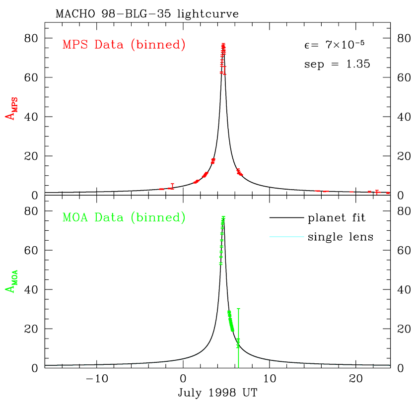
Figure 1: The light curves of the MPS and MOA data sets are plotted as a function of time with the best fit planetary and single lens light curves (which are nearly indistinguishable in this Figure. The data are binned and averaged on 0.03 day intervals, but the fits shown are the best fits to the unbinned data.

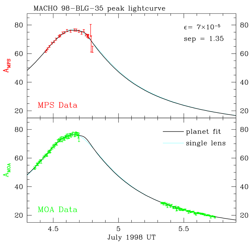
Figure 2: A close-up view of the MPS and MOA light curves near peak magnification. The best fit planetary and single lens light curves can be distinguished near peak magnification. The data are not binned.

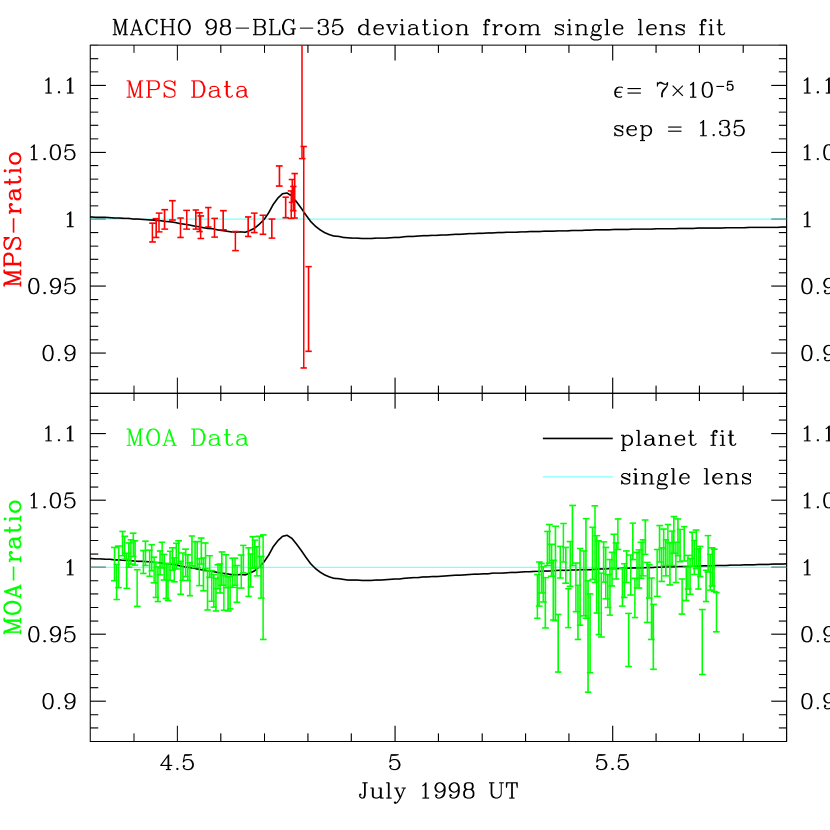
Figure 3: The ratio of the data and the best fit planetary lensing light curve to the best fit single lens light curve are plotted as a function of time. The differences between the MPS and MOA fit light curves are due to the different amounts of lensed and unlensed flux in the different fits.

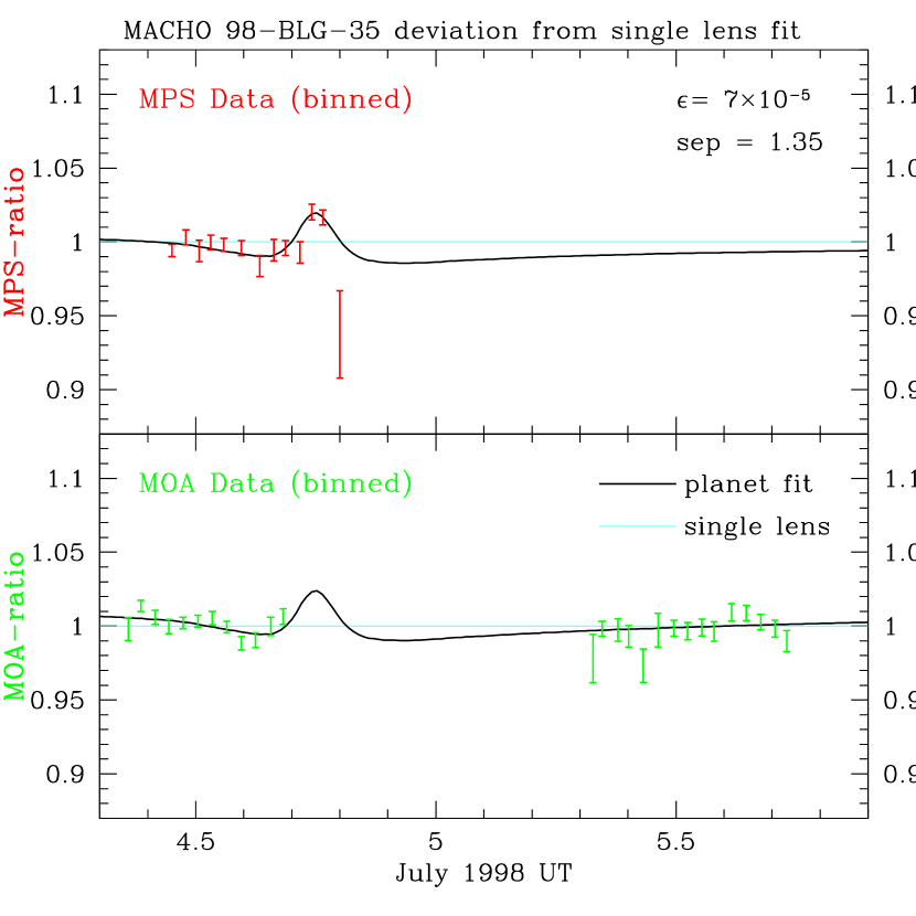
Figure 4: The same as Figure 3, but with data binned and averaged on 0.03 day intervals. The the microlensing fits have all been done with the unbinned data.

The parameters for three fit planetary microlensing light curves and the best fit single lens light curve are presented in Tables 1-3. Figures 1-4 show a comparison of the best fit planetary lens light curve to the best fit single light curve. Figures 1 and 2 show the data along with these two light curves, while Figures 3 and 4 show the light curves and data divided by the best fit single lens light curve. Because of the high frequency of observations, the data shown in Figures 1 and 4 have been averaged into 0.03-day long bins. This binning is for display purposes only. All the fits have been done to the full data set. The best fit light curve has a mass fraction of $\epsilon=7\times 10^{-5}$ and has a $\chi^{2}$ improvement over the single lens fit of 23. This improvement in $\chi^{2}$ (with three additional parameters) implies that the planetary “detection” is significant at the $4.5\sigma$ level. This improvement in $\chi^{2}$ appears to be evenly divided between the MPS and MOA data.

The best fit $\chi^{2}=303.4$ for 275 degrees of freedom for the best fit planetary lens curve. The probability for a $\chi^{2}$ value at least this large is about 12% assuming the model is correct. For the best fit single lens curve, $\chi^{2}$ is larger by 23, but there are 3 more degrees of freedom because the model has fewer parameters. The probability of a $\chi^{2}$ value this large to occur by chance is only 2.4%.

The fit $\chi^{2}$ is somewhat worse for the MPS data: $\chi^{2}=156.1$ for 118 degrees of freedom (assuming that 5 of the 10 fit parameters can be associated with the MPS data). The probability that a $\chi^{2}$ value this large will occur by chance is only about 1%. However, there is one MPS observation from July 16 that contributes 19 to the $\chi^{2}$ value. If this point is excluded, then the $\chi^{2}$ probability increases to 10%. This suggests that it is probably reasonable to use the SoDOPHOT and DOPHOT generated error estimates.

Tables 1-3 also present the fit parameters and $\chi^{2}$ values for both a “low mass” and “high mass” planetary fit in addition to the best fit. These fits have $\chi^{2}$ values that are larger than the best fit by about 4, so they correspond to approximate $2\sigma$ limits on the planetary mass fraction. Thus, the $2\sigma$ constraint on $\epsilon$ is $1.7\times 10^{-5}<\epsilon<7\times 10^{-4}$. The $1\sigma$ limits are $4\times 10^{-5}<\epsilon<2\times 10^{-4}$. For a likely primary lens mass of 0.1-0.6$\rm{M_{\odot}}$, the $1\sigma$ range of planetary masses extends from about an Earth mass to twice the mass of Neptune. Table 2 indicates that the MPS data prefer a lower planetary mass while the MOA data would prefer a somewhat higher planetary mass.

Another apparent difference between the MPS and MOA data can be seen in Table 3 which gives the best fit lensed ($F_{\ell}$) and unlensed ($F_{u}$) source flux values for each fit. These are given in instrumental units, and it is necessary to include these parameters because of the high stellar density in the fields where microlensing events are observed. It is often the case that the stellar “objects” detected by the photometry codes will actually consist of several stars which are within the same seeing disk. Only one of these stars will be lensed at a time, so it will appear that only part of the flux of these stellar “objects” is lensed. In the case of MACHO-98-BLG-35, the MPS template frame was taken when the source was magnified by about a factor of three, and the MPS photometry code found three “objects” with a brightness comparable to the unlensed brightness of the source within 2.5${}^{\,\prime\prime}$ of the source “object.” These “objects” were not separately resolved in the MOA template image which was taken when the source was magnified by a factor of 60. Presumably, these stars were lost in the wings of the lensed source. This probably accounts for the fact that the lensed flux ($F_{\ell}$) is about 92% of the total flux for the MPS data but only 66% of the total flux for the MOA data.

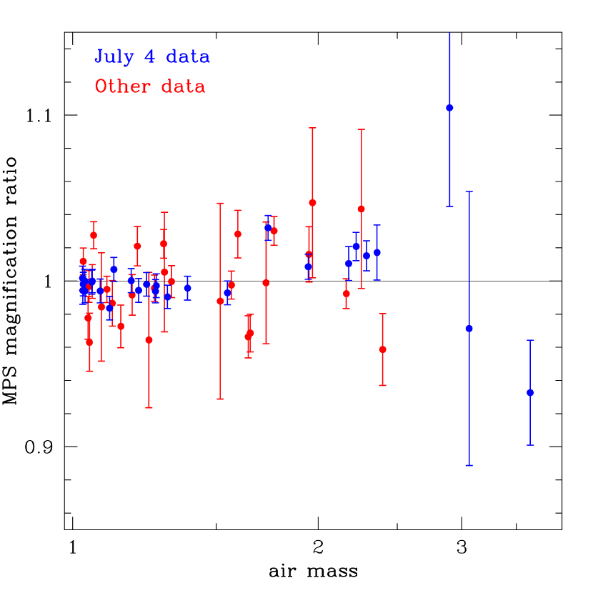
Figure 5: The magnification ratio from the best fit single lens light curve is plotted as a function of airmass for the MPS data taken within the week centered on the time of maximum magnification. The data from the night of the planetary signal (July 4) are plotted in blue while the other data are plotted in red.

The light curve features that are responsible for this apparent planetary detection can be seen most easily in Figures 3 and 4. The most significant deviations from the best single lens fit are the 1.5% decrease in flux relative to the single lens fit between July 4.34 and July 4.64 and then an increase of about 3% to a relative maximum at about July 4.75. The slight flattening of the peak relative to the single lens fit seen in Figurefig-lc2d appears as the systematic trend of declining from July 4.34 to July 4.64. The increase of the flux seen in MPS data at about July 4.75 is the sharpest feature seen in the light curve, and it occurred while the source was setting from Mt. Stromlo. The observations in the peak of this feature were taken at an airmass ranging from 1.7 to 2.4 which is higher than most of our observations. (The final three observations had an airmass range of 2.8 to 3.6, but the observations provide little weight to the planetary signal.) Figure 5 shows the dependence of the magnification ratio on airmass for the MPS data taken in the week centered on the peak magnification for this event. There is a slight excess of observations at an airmass $\sim 2$ with a magnification ratio $>1$, but as the color coding of the points indicates, this is due to the fact that a large fraction of these observations were taken during the light curve deviation on July 4. Aside from this, there is no obvious trend with airmass, which suggests that the feature seen in the MPS data is not a systematic error due to the higher than average airmass of the observations. A discussion of the photometric accuracy of the MOA data can be found in an article by Yock Yock (1999).

In addition to the planetary fits presented in Tables 1-3, there is also a set of fits with parameters very nearly identical to those in Table 1 except with the planetary separation replaced by its inverse: $a\rightarrow 1/a$. This is the well known “duality” feature Griest & Safizadeh (1998) of the central caustic for planetary lensing events, and it gives rise to a substantial uncertainty in the separation of the planet from the lens. The best fit planetary lens models have $a=1.35$ and $a=1/1.35$, but $a=1.45$ and $a=1/1.45$ are consistent at $1\sigma$ while $a=2.07$ and $a=1/2.07$ are consistent at a $2\sigma$ confidence level.

We should also consider the possibility that the light curve deviation is caused by something other than a planet. For example, it is possible to get a bump on the light curve from a binary source star lensed by a single lens Gaudi (1998). Since the observed feature has a timescale about a factor of ten shorter than the overall event timescale and an amplitude of about 3% of the peak magnification, it might be possible to have a similar light curve if the source star has a companion about 6 magnitudes fainter which has a peak magnification 10 times larger than the factor of 80 observed for the primary source star. This would give these observed features if the separation of two sources on the sky was about 0.012 Einstein radii. For typical lens parameters and a random orientation of the source system orbit, this gives a semi-major axis of 0.05 AU.

However, if the source star is in a short period binary system, then the trajectory of the source with respect to the lens system will not be a straight line. The orbital motion of the source will generate a wobble in the source trajectory which will cause periodic variations in the light curve Han & Gould (1997). No such variations are seen, and this puts strong constraints on the nature of possible binary parameters of the source star. These variations may not be seen if the orbital period of the binary source is larger than the timescale of the lensing event, but this would require that the source orbit be nearly edge on and that the two sources be just passing each other at the time of peak magnification in order to reproduce such a light curve. In addition, a secondary source 6 magnitudes fainter than the primary would probably have a very different color. Although MPS and MOA have little color information for this event, other groups such as MACHO and PLANET have observed it in different color bands. In short, it would seem to require several unlikely coincidences to have a binary source event mimic a planetary perturbation in this case. A future analysis including data from MACHO and PLANET may be able to rule out this possibility.

4.2 Planetary Limits

One of the benefits of these high magnification microlensing events is that planets can be detected with high efficiency at a large range of orbital separations around the lens star. This means that the absence of a strong planetary signal can be used to place limits on the possible planets of the lens system. We have used the following procedure to quantify these limits. We consider a dense sampling of the planetary lens parameter space with the planetary separation, $a$, spanning the range from $0.2$ to $7$ with an interval of $0.02$, $\theta$ varying from 0 to $2\pi$ at intervals of $1^{\circ}$, and $\epsilon$ ranging from $3\times 10^{-7}$ to $10^{-2}$ in logarithmic intervals of $10^{1/8}=1.33$. The other parameters were fixed so as to be quite close to the observed values ($t_{\rm 0}=4.65$ July UT, $t_{E}=20\,$days, and $u_{\rm min}=0.0125$).

For each set of parameters, an artificial light curve was created and imaginary observations were performed at the same times and with the same error bars as the actual MPS and MOA observations. The resulting artificial data set was then fit with a 7-parameter single lens model, and the best fit $\chi^{2}$ value was determined. Since no photometric noise was added to these light curves, the fit $\chi^{2}$ values should be $<1$ for events that are indistinguishable from single lens events (at $1\sigma$ confidence) or $>1$ otherwise. The addition of Gaussian photometric noise should just add a contribution to $\chi^{2}$ equal to the number of degrees of freedom, so our measured $\chi^{2}$ values should be considered to be the additional $\Delta\chi^{2}$ contribution caused by the planetary signal. We set a detection threshold of $\Delta\chi^{2}\geq 40$ which corresponds to a $6.3\sigma$ deviation from the best fit single lens light curve. Thus, we take each set of planetary parameters that give best fit single lens curves with $\Delta\chi^{2}\geq 40$ to indicate that these planetary parameters have been ruled out. The threshold of $\Delta\chi^{2}\geq 40$ was selected to be somewhat larger than the deviation that we have actually detected in the light curve.

All of these calculations were done using a point-source approximation to calculate the planetary lensing light curves. This approximation is accurate for most of the light curves, but some of the light curves will include caustic crossings which would require a much more time consuming finite source light curve calculation which would be complicated by the fact that we do not know what the source size actually is. A reasonable estimate for the source size projected to the plane of the lens system is $\hbox{ \hbox to0.0pt{\raise 1.82986pt\hbox{$<$}\hss}\lower 2.79857pt\hbox{$\sim$} }0.004\,R_{E}$, so finite source effects are probably not very large. We have repeated our calculations for finite sources with a much sparser sampling of the planetary lensing parameters. These calculations indicate that the point source calculations slightly underestimate the planetary detection probability for $\epsilon>10^{-5}$, but they overestimate the planetary detection probability for $\epsilon\hbox{ \hbox to0.0pt{\raise 1.82986pt\hbox{$<$}\hss}\lower 2.79857pt\hbox{$\sim$} }10^{-5}$. Thus, our limits are conservative for $\epsilon>10^{-5}$, but they may be overoptimistic for $\epsilon\hbox{ \hbox to0.0pt{\raise 1.82986pt\hbox{$<$}\hss}\lower 2.79857pt\hbox{$\sim$} }10^{-5}$.

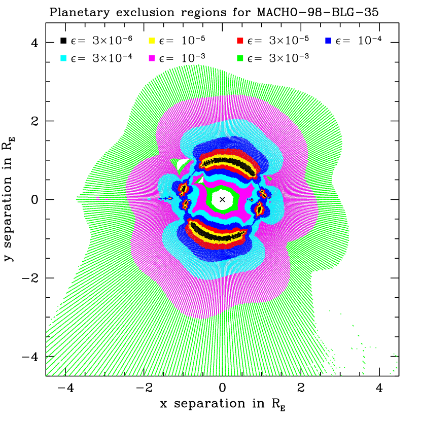
Figure 6: The excluded region of the lens plane is shown for a range of planetary mass fractions ranging from $\epsilon=3\times 10^{-6}$ to $\epsilon=3\times 10^{-3}$.

Figure 6 shows the regions of the lens plane where planets are excluded for various planetary mass fractions ranging from $\epsilon=3\times 10^{-6}$ to $\epsilon=3\times 10^{-3}$. During the lensing event, the source star crosses from right to left on the x-axis. The gaps in the shaded regions represent our lack of sensitivity to planets at particular $\theta$ angles where the planetary light curve deviation occurs at a time when we have poor coverage of the microlensing light curve.

Theoretical papers on the microlensing planet search technique have generally asserted that microlensing can detect planets that are in the so-called “lensing zone” which covers the range $0.6<a<1.6$ Gould & Loeb (1992); Bennett & Rhie (1996); Griest & Safizadeh (1998), but the exclusion regions for $3\times 10^{-4}\leq\epsilon\leq 3\times 10^{-3}$ in Figure 6 clearly extend far beyond this region Rhie & Bennett (1996). There are also significant exclusion regions for $\epsilon=3\times 10^{-6}$ and $\epsilon=10^{-5}$ which correspond to planets of about an Earth mass, so this event represents the first observational constraints on Earth-mass planets orbiting normal stars.

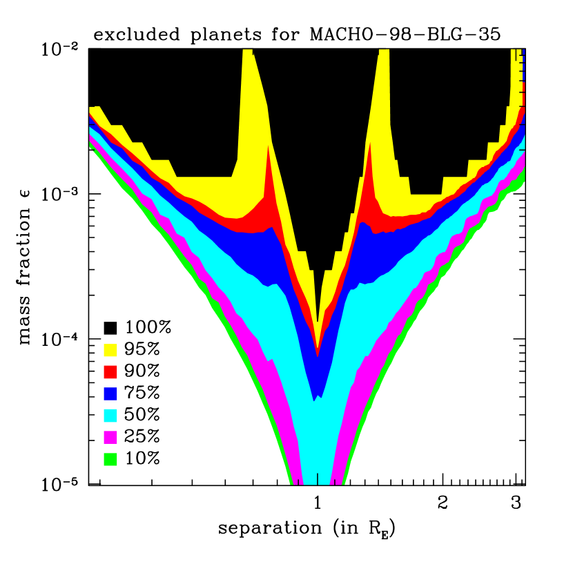
Figure 7: The parameters of planets excluded from the MACHO-98-BLG-35 system are shown in the mass fraction - separation plane. The different colors indicate what fraction of the planets with the given mass fraction and separations are excluded.

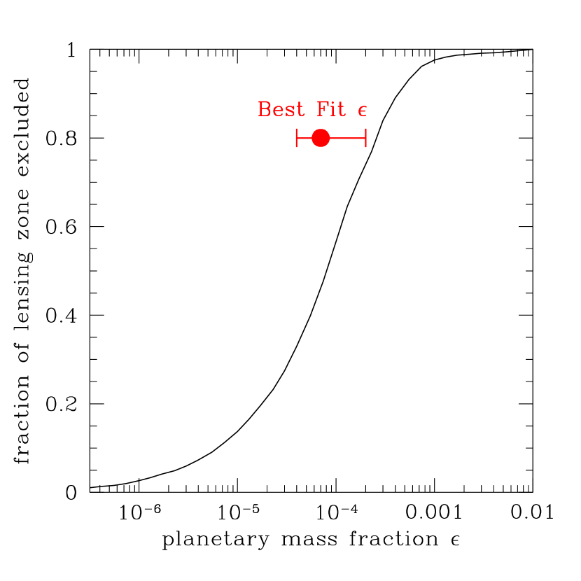
Figure 8: The fraction of the lensing zone, $0.6\leq R_{E}\leq 1.6$, where planets are excluded from the MACHO-98-BLG-35 system is plotted as a function of the mass fraction $\epsilon$. The best fit mass fraction is shown for comparison (plotted at an arbitrary $y$-axis value).

Another view of the planetary constraints can be seen in Figures 7-8. In Figure 7, we have averaged over all the $\theta$ values, and we show the contours of the regions excluded at various confidence levels in the $a$-$\epsilon$ plane. The $x$-axis of Figure 7 is plotted on a logarithmic scale which reveals an approximate reflection symmetry about $a=1$. This is an indication of the dual $a\rightarrow 1/a$ symmetry of light curves which approach the stellar caustic. We make use of this duality property to construct Table 4 which gives 50% and 90% confidence level exclusion ranges for the planetary separation, $a$, as a function of the planetary mass fraction, $\epsilon$. The limits of the planetary separation exclusion ranges are chosen to be related by the $a\rightarrow 1/a$ transformation. Table 4 indicates that Jupiter-like planets ($\epsilon\geq 10^{-3}$) are excluded from a region much larger than the usual lensing zone, while planets with $\epsilon\geq 3\times 10^{-5}$ (several Earth masses or more) are excluded from a large fraction of the lensing zone.

Because of the enhanced planetary detection probability in the lensing zone Gould & Loeb (1992); Bennett & Rhie (1996); Griest & Safizadeh (1998), it is instructive to consider the fraction of the lensing zone from which planets are excluded as a function of mass fraction, $\epsilon$. This is plotted in Figure 8, and the $\epsilon$ range for our apparent planetary detection is shown as well. This figure shows that the majority of the lensing zone must be free of planets for $\epsilon\hbox{ \hbox to0.0pt{\raise 1.82986pt\hbox{$>$}\hss}\lower 2.79857pt\hbox{$\sim$} }10^{-4}$, while more than 97% of the lensing zone can have no planets with $\epsilon\hbox{ \hbox to0.0pt{\raise 1.82986pt\hbox{$>$}\hss}\lower 2.79857pt\hbox{$\sim$} }10^{-3}$. At $\epsilon\sim 10^{-5}$, which corresponds to an Earth mass, more than 10% of the lensing zone is excluded.

This relatively high planet detection probability is a feature of high magnification events that was first emphasized by ?). The planet causes a distortion of the stellar caustic which can be seen in the light curves of high magnification events for a large range of planetary parameters, as we have shown. However, when only the stellar caustic is detected, the determination of the planetary lens parameters can be somewhat ambiguous if the planetary signal is not very strong.

Most of the detectable planetary microlensing signals are due to planetary caustics, and for these events, one can determine $\epsilon$ and $a$ from the timing and the magnification of the stellar peak with respect to the planetary deviation of the lightcurve Gould & Loeb (1992); Bennett & Rhie (1996); Gaudi & Gould (1997). The planetary caustics cover a larger area of the lens plane than the stellar caustic does, hence one expects a higher probability of a planetary discovery for a planetary caustic event over a stellar caustic event. However, the stellar caustic events have observational advantage that the timing of the stellar caustic approach or crossing can be predicted ahead of time which allows the scheduling of additional observations that can greatly increase the planetary detection probability.

4.3 Solar System Analogs

Thus far, we have discussed the limits placed on the planetary system of the MACHO-98-BLG-35 lens star in terms of the units which are the most convenient in the context of gravitational microlensing. We have talked about the “lensing zone” and used $R_{E}$ as our basic unit of distance. Since these are the natural units of microlensing, this allows us to be precise and economical in our discussion of the limits, but they are not the units that we usually use to measure solar systems. Although $R_{E}$ is typically of order an AU, it does have a rather broad distribution. Thus, it might be easier to see the significance of our limits if we translate them into solar system units. To accomplish this, let us consider the possibility that the lens system is a solar system analog. What are the chances that we would have detected a light curve deviation with $\Delta\chi^{2}>40$ if the lens star has a solar system just like that of the Sun?

In order to answer this question, we need to average over the parameters of the lens system that are unknown. These include: the lens and source distances, the inclination of the lens star’s planetary plane, and the position of each planet in its orbit. Also, since the lens star’s mass is likely to be less than a solar mass, we need a prescription for how the planetary separations scale with the mass of the lens star. In order to simplify our calculations, we assume that the planetary separations scale as $M^{1/2}$, but this does not have a large influence on our results. (We continue to refer to planetary separations in AU, but it should be understood that these distances are scaled as $M^{1/2}$. Thus, the “Jupiter” of a planetary system orbiting a $0.3\rm{M_{\odot}}$ star would be at a orbital distance of 2.8 AU.) We also assume that the distribution of fractional planetary masses does not depend on the mass of the lens star. This means that our “Jupiter” will always have a mass fraction of $\epsilon=10^{-3}$ independent of the lens mass. We should also point out that our calculations are not strictly correct for systems with more than one planet, since we have only done calculations for binary lens systems. We have assumed that each planet can be detected only if it could be detected in the same position in a purely binary system. In practice, the additional lenses may increase the light curve deviations for events near the detection threshold and push these events above the detection threshold. So, our simplification probably causes a slight underestimate of the planetary detection probability.

Applying this procedure to our MACHO-98-BLG-35 data, we find that a Solar System analog is excluded at the 90% confidence level. In 88% of the cases, the Jupiter-like planet ($\epsilon=10^{-3}$ at 5.2 AU) would be detected, and the Saturn-like planet ($\epsilon=3\times 10^{-4}$ at 9.5 AU) would be detected 19% of the time although the Jupiter would be also seen in most of these cases. About 1% of the time the Earth, Uranus or Neptune analogs would be seen.

If we modify the Solar System analog to replace the Jupiter-like planet with a Saturn mass planet ($\epsilon=3\times 10^{-4}$) at 5.2 AU, we find that this system can be excluded at 69% confidence. The Saturn in Jupiter’s orbit is seen 64% of the time while both Saturns can be detected in about 15% of the cases.

Finally, let us consider planetary systems in which Jupiter and Saturn have been replaced by Neptune-like planets with $\epsilon=5\times 10^{-5}$. This is a planetary configuration suggested by ?) based on consideration of planet formation theory, and following Peale, we also introduce an additional Earth at 2.5 AU because the formation of such a planet would be expected if Jupiter were absent. We find that there is a 36% chance that such a low mass planetary system would give rise to an unacceptably large signal and be excluded by our data. About 29% of the time, the Neptune at Jupiter’s position would be seen while the Neptune in Saturn’s orbit would be seen 4.5% of the time and the Earth at 2.5 AU would be seen 2.5% of the time. As with the solar system analog, the remaining planets contribute about 1% of the total detection probability. While the exclusion of such planetary systems at 36% confidence is not a very significant result by itself, it does indicate that with a few more similar data sets, we will begin to be able to address the question of the abundance of planetary systems without gas giants. Of course, the apparent planetary signal in our data is consistent with the detection of just such a system, so it is quite possible that we have made the first detection of a planet in a system with no gas giants.

5 Discussion and Conclusion

Our 90% confidence level exclusion of a Solar System analog planetary system is apparently the tightest constraint on planetary systems like our own to date. The radial-velocity program of Marcy and Butler has one or two systems in which they can constrain $\epsilon\sin i<10^{-3}$ Marcy (1999) at present. This is comparable to our constraint except for the additional uncertainty due to the unknown inclination angle, $i$. However, their current radial-velocity sensitivity is good enough to obtain similar limits for hundreds of stars once they have high sensitivity observations spanning the decade-long orbital periods of planets at 5 AU. So, within a few years, the radial-velocity groups will likely have similar constraints for hundreds of stars.

The real strength of the microlensing technique lies not with the ability to detect Jupiter analogs, but in the sensitivity to lower mass planets. Of course, low mass planets are more difficult to see with any technique, but with microlensing the planetary signals do not get substantially weaker as the planetary mass drops as they do for other techniques. Instead, the microlensing signatures of extra-solar planets become rarer and briefer as the planetary mass decreases down to $\epsilon\sim 10^{-5}$ where finite source effects become important. If we had 10 microlensing events with limits similar to MACHO-98-BLG-35, then our statistical information on the prevalence of Jupiter-like planets would be interesting, but probably not competitive with what will be learned from the radial-velocity searches. However, we would expect to detect several Neptune-mass planets with a signal substantially stronger than the planetary signal seen in our MACHO-98-BLG-35 data if most planetary systems have Neptune-mass planets. Our sensitivity to Neptune and probably Saturn-mass planets would very likely be beyond the sensitivity of the radial-velocity searches or other ground based planet search techniques. So, if it were the case that most planetary systems have no planets more massive than Neptune, gravitational microlensing would likely be the only ground based planet search technique sensitive to these planetary systems.

Our planetary results for event MACHO-98-BLG-35 have made use of the large planet detection efficiency for high magnification microlensing events that was first emphasized and quantified by ?). Although there are probably more detectable planetary signals for low magnification events, the high magnification events have the advantage that the planetary signal is expected near the time of peak magnification which can be predicted with relatively sparse observations (once, or preferably, a few times per day). If the light curve is then sampled very frequently near peak magnification, there will be a high probability of detecting a planet. The light curve can be sampled more sparsely after the magnification decreases. Because we know when the planetary signal is likely to occur, it is possible to discover a low mass planet with a relatively small total number of observations. It is critical, however, that the high magnification events be discovered in advance and that they be observed frequently enough to predict their peak magnification.

Let us consider the recent history of microlensing events discovered in real time. The MACHO alert system has found 4 microlensing events with a peak magnification $>20$, in addition to a number of high magnification binary lensing events with large mass fractions ($\epsilon>0.1$). The high magnification events are MACHO-95-BLG-11, MACHO-95-BLG-30, MACHO-98-BLG-7, and MACHO-98-BLG-35. OGLE has also found 4 such events: OGLE-98-BUL-29, OGLE-98-BUL-32, OGLE-98-BUL-36 , and OGLE-99-BUL-5. Of these events, only MACHO-95-BLG-30 Alcock et al. (1997), MACHO-98-BLG-35, and OGLE-99-BUL-5 were discovered substantially before peak magnification, while MACHO-95-BLG-11 and OGLE-98-BUL-29 were discovered in the 24-hour period preceding peak magnification. Any steps that might be taken towards earlier discovery of microlensing events in progress are likely to improve the planet detection efficiency significantly. It is also critical that detected events be observed frequently enough to predict high magnification events reliably.

The high efficiency for planet detection for this event and the uncertainty in the planetary lensing parameters are both consequences of the very high magnification of lensing event MACHO-98-BLG-35. More accurate planetary parameters can be obtained for events where the planetary caustic is crossed or approached, which generally occurs at a more modest magnification. Detectable light curve deviations caused by an approach to the planetary caustic are more frequent than light curve deviations caused by an approach to the stellar caustic, but we cannot predict in advance when a planetary caustic might be approached so it requires more telescope time to find such events. Dedicated microlensing follow-up programs such as those being run by PLANET Albrow et al. (1998) and MPS, are required in order to have a reasonable prospect of detecting such events. However, despite the complete longitude coverage of the PLANET collaboration and the 1.9m telescope used by MPS, the current generation of microlensing planet search programs is not able to follow enough microlensing events with sufficient photometric accuracy to obtain statistically significant constraints on the abundance of low mass planets. This would require a more ambitious microlensing follow-up program along the lines of that presented by ?).

In summary, we have presented the first observational constraints on a planetary system from gravitational microlensing, including a $4.5\sigma$ detection of an apparent planetary signal. The mass fraction of this planetary companion to the lens star is likely to be in the range $4\times 10^{-5}\leq\epsilon\leq 2\times 10^{-4}$. Depending on the lens star mass, these mass fractions correspond to planetary masses in the range from a few Earth masses up to about two Neptune masses. Our data also place strong constraints on the planetary system which may orbit the lens star. A system just like our own is excluded at 90% confidence while a system like ours with Jupiter replaced by a Saturn-mass planet can be excluded at 70% confidence. For a planetary system like our own with Jupiter and Saturn replaced by Neptunes we would expect a signal at least twice as strong as the one that we have detected about 30% of the time. Our results demonstrate the sensitivity of the gravitational microlensing technique to low mass planets. If we take our low mass planet detection at face value, then it suggests that the most common planetary systems in the Galaxy may be the ones with their most massive planets less massive than a gas giant.

Table 1: Binary lensing parameters and statistics

parameter	single lens	best fit	low mass	high mass
$t_{\rm 0}$ (July UT)	4.65(9)	4.65(9)	4.65(9)	4.66(9)
$t_{E}$ (days)	21.13(56)	21.45(22)	21.49(21)	21.25(27)
$u_{\rm min}$	0.01322(38)	0.01299(14)	0.01296(13)	0.01208(16)
$a$	0	1.35(3)	1.19(2)	2.07(8)
$\theta$ (rad)	0	1.94(4)	1.91(3)	2.17(3)
$\epsilon$	0	$7.0(1.5)\times 10^{-5}$	$1.7\times 10^{-5}$	$7.0\times 10^{-4}$
$\chi^{2}/$ (d.o.f)	326.45/278	303.44/275	307.04/275	307.65/275

Table 2: Fit $\chi^{2}$ values for individual data sets

data set	single lens	best fit	low mass	high mass
MPS R	170.40/123	157.25/123	156.13/123	163.16/123
MOA red	156.06/162	146.19/162	150.91/162	144.49/162

Table 3: Lensed and unlensed fluxes ($F_{\ell}$ & $F_{u}$)

data set	single lens	best fit	low mass	high mass
MPS R $F_{\ell}$	199.2(4)	195.4(4)	194.9(4)	197.0(4)
MPS R $F_{u}$	13.6(1.4)	16.5(1.4)	17.2(1.4)	16.3(1.4)
MOA red $F_{\ell}$	287.1(7)	282.5(7)	281.0(7)	283.6(7)
MOA red $F_{u}$	115(23)	147(23)	155(23)	199(23)

Table 4: Planetary exclusion regions

mass fraction: $\epsilon$	90% excluded	50% excluded
$3\times 10^{-3}$	$0.27\leq a\leq 3.70$	$0.16\leq a\leq 6.25$
$10^{-3}$	$0.37\leq a\leq 2.70$	$0.22\leq a\leq 4.55$
$3\times 10^{-4}$	$0.74\leq a\leq 1.35$	$0.39\leq a\leq 2.56$
$10^{-4}$	$0.94\leq a\leq 1.06$	$0.58\leq a\leq 1.72$
$3\times 10^{-5}$	$-$	$0.76\leq a\leq 1.31$
$10^{-5}$	$-$	$0.88\leq a\leq 1.13$
$3\times 10^{-6}$	$-$	$0.98\leq a\leq 1.02$

References

- Abe et al. (1999) Abe, F. et al. 1999, AJ, in press
- Albrow et al. (1998) Albrow, M., et al. 1998, ApJ, 509, 687
- Alcock et al. (1996) Alcock, C., et al. 1996, ApJ, 463, L67
- Alcock et al. (1997) Alcock, C., et al. 1997, ApJ, 491, 436
- Alcock et al. (1999) Alcock, C., et al. 1999, PASP, submitted
- Allen, Peterson & Shao (1997) Allen, R. J., Peterson, D. M. & Shao, M. 1997, Proc. SPIE, 2871, 504
- Beichman (1998) Beichman, C. A. 1998, Proc. SPIE, 3350, 719
- Bennett et al. (1993) Bennett, D. P., et al. 1993, American Astronomical Society Meeting, 183, 7206
- Bennett & Rhie (1996) Bennett, D. P., & Rhie, S. H. 1996, ApJ, 472, 660
- Bolatto & Falco (1994) Bolatto, A. D. & Falco, E. E. 1994, ApJ, 436, 112
- Di Stefano & Scalzo (1999) Di Stefano, R., & Scalzo, R. 1999, ApJ, 512, 564
- Di Stefano & Scalzo (1999) Di Stefano, R., & Scalzo, R. 1999, ApJ, 512, 579
- Elachi et al. ( 1996) Elachi, C. , et al. 1996, Jet Propulsion Lab. Report
- Gaudi (1998) Gaudi, B. S. 1998, ApJ, 506, 533
- Gaudi & Gould (1997) Gaudi, B. S. & Gould, A. 1997, ApJ, 486, 85
- Gaudi et al. (1998) Gaudi, B. S., et al. 1998, American Astronomical Society Meeting, 193, 110807
- (17) Gaudi, B. S., Naber, R., & Sackett, P. 1998, ApJ, 502, L33
- Gould & Loeb (1992) Gould, A. & Loeb, A. 1992, ApJ, 396, 104
- Griest & Safizadeh (1998) Griest, K. & Safizadeh, N. 1998, ApJ, 500, 37
- Han & Gould (1997) Han, C. & Gould, A. 1997, ApJ, 480, 196
- Honeycutt (1992) Honeycutt, R. K. 1992, PASP, 104, 435
- Koch et al. (1998) Koch, D. G., Borucki, W. , Webster, L. , Dunham, E. , Jenkins, J. , Marriott, J. & Reitsema, H. J. 1998, Proc. SPIE, 3356, 599
- Mao & Paczynski (1991) Mao, S., & Paczynski, B. 1991, ApJ, 374, L37
- Marcy (1999) Marcy, G. W. 1999, private communication.
- Marcy & Butler (1998) Marcy, G. W. & Butler, R. P. 1998, ARA&A, 36, 57
- Padgett et al. (1999) Padgett, D. L., Brandner, W. , Stapelfeldt, K. R., Strom, S. E., Terebey, S. & Koerner, D. 1999, AJ, 117, 1490
- Peale (1997) Peale, S. J. 1997, Icarus, 127, 269
- Penny et al. (1998) Penny, A. J., Leger, A., Mariotti, J.-M. , Schalinski, C., Eiroa, C., Laurance, R. J. & Fridlund, M. 1998, Proc. SPIE, 3350, 666
- Reid, Dodd & Sullivan (1998) Reid, M. L., Dodd, R. J. & Sullivan, D. J. 1998, AJA, 7, 79-85
- Rhie et al. (1999) Rhie, S. H., Becker, A. C., Bennett, D. P., Fragile, P. C., Johnson, B. R., King, L., Peterson, B. A. & Quinn, J. 1999 ApJ, in press (astro-ph/9812252)
- Rhie & Bennett (1996) Rhie, S. H., and Bennett, D. P. 1996, Nucl.Phys.Proc.Suppl. 51B, 86-90
- Schechter, Mateo & Saha (1993) Schechter, P. L., Mateo, M. & Saha, A. 1993, PASP, 105, 1342
- Schlegel, Finkbeiner & Davis (1998) Schlegel, D. J., Finkbeiner, D. P. & Davis, M. 1998, ApJ, 500, 525
- Stanek (1999) Stanek, K. Z. 1999, ApJ, submitted (astro-ph/9802307)
- Wambsganss (1997) Wambsganss, J. 1997, MNRAS, 284, 172
- Wolszczan & Frail (1992) Wolszczan, A. & Frail, D. A. 1992, Nature, 355, 145
- Yock (1999) Yock, P. 1999, astro-ph/9908198