CFNUL - 99/03
Velocity at the Schwarzschild horizon revisited

Abstract

The question of the physical reality of the black hole interior is a recurrent one. An objection to its existence is the well known fact that the velocity of a material particle, refered to the stationary frame, tends to the velocity of light as it approaches the horizon.

It is shown, using Kruskal coordinates, that a timelike radial geodesic does not become null at the event horizon.

The interpretation of the maximal analytic extension of the 4 regions Schwarzschild spacetime presents some difficulties. The conventional view is that the only regions relevant to a black hole formed by gravitational collapse are regions I and II [1].

There is however a long list of literature where the physical reality of the black hole interior (region II) is argued. References can be found elsewhere [2].

Recently a new case was made to that point [3]. There, the reasoning is mainly based in the result that the velocity of any material particle as measured by a Kruskal observer (as defined below) is equal to 1 at the event horizon. The purpose of this paper is to show that this is not the case.

In Schwarzschild coordinates, the metric of the Schwarzschild spacetime takes the well known form,

$$ds^{2}=-\left({1-{{2m}\over r}}\right)dt^{2}+\left({1-{{2m}\over r}}\right)^{-1}dr^{2}+r^{2}\left({d\theta^{2}+\sin^{2}\theta d\varphi^{2}}\right).$$ (1)

For $r>2m$, the Kruskal coordinates $(x^{\prime},t^{\prime})$ relate to these by,

$$\left\{\begin{array}[]{lll}\mbox{$x^{\prime 2}-t^{\prime 2}=\left({{{r-2m}\over{2m}}}\right)e^{r/2m}$}\\ \\ \mbox{$t^{\prime}=\tanh\left({{t\over{4m}}}\right)x^{\prime}$}\end{array}\right.$$ (2)

In these coordinates the metric takes the form [4],

$$ds^{2}={{32m^{3}}\over{r}}e^{-r/2m}(-dt^{\prime 2}+dx^{\prime 2})+r^{2}\left({d\theta^{2}+\sin^{2}\theta d\varphi^{2}}\right).$$ (3)

A Kruskal observer is one which maintains the space-like coordinate $x^{\prime}$ constant and consequentely, from (3), it verifies,

$${{32m^{3}}\over{re^{r/2m}}}\left({{{dt^{\prime}}\over{d\tau}}}\right)^{2}=1.$$ (4)

Differentiating (2) we get,

$${{{dr}\over{d\tau}}}={{8m^{2}}\over{e^{r/2m}r}}\left(x^{\prime}{{{dx^{\prime}}\over{d\tau}}}-t^{\prime}{{{dt^{\prime}}\over{d\tau}}}\right), {{dt}\over{d\tau}}=\left({x^{\prime}{{dt^{\prime}}\over{d\tau}}-t^{\prime}{{dx^{\prime}}\over{d\tau}}}\right){{8m^{2}}\over{e^{r/2m}(r-2m)}}.$$ (5)

Using $dx^{\prime}=0$ and (4) we can write the following equation :

$$\left({1-{{2m}\over r}}\right)\left({{{dt}\over{d\tau}}}\right)^{2}-\left({1-{{2m}\over r}}\right)^{-1}\left({{{dr}\over{d\tau}}}\right)^{2}={{2m(x^{2}-t^{2})}\over{e^{r/2m}(r-2m)}}=1,$$ (6)

meaning the Kruskal observer follows a radial trajectory.

Consider now a material particle along a radial ingoing trajectory in region I. Its velocity, measured by a Kruskal observer is simply

$$v={{dx^{\prime}}\over{dt^{\prime}}},$$ (7)

since (3) is diagonal with $g_{x^{\prime}x^{\prime}}=-g_{t^{\prime}t^{\prime}}$. Dividing one of the equations (5) by the other and solving for $v$ we obtain,

$$v={{1+t^{\prime}/x^{\prime}{{dt}\over{dr}}(1-2m/r)}\over{t^{\prime}/x^{\prime}+{{dt}\over{dr}}(1-2m/r)}},$$ (8)

which is the equation (20) of [3].

At the event horizon, separating regions I and II, the coordinates take the values: $r=2m$, $t=+\infty$, $t^{\prime}/x^{\prime}=\tanh(t/4m)=1$ and $x^{\prime}\neq 0$. Apparently, making $t^{\prime}/x^{\prime}=1$ shows that when the particle, following any trajectory described by $dt/dr$, and the observer intersects at the horizon, the velocity measured by the latter is 1. However, $v$ is a function of 2 coordinates ($r$ and $t$), and both limits must be taken simultaneously.

To illustrate this point, consider the movement of a particle $p$ in special relativity, relative to 2 referencials $S$ and $S^{\prime}$ with all the movements parallel to each other. The well known expression for the addition of velocities is,

$$v^{\prime}_{p/S^{\prime}}=\left({{v_{p/S}-V_{S^{\prime}/S}}\over{1-v_{p/S}V_{S^{\prime}/S}}}\right).$$ (9)

If both particle and $S^{\prime}$ are moving at the speed of light with respect to $S$, their relative velocity is not necessarily 1, the expression giving ${0\over 0}$. However, if we take only the limit $v_{p/S}=1$ we obtain identical expressions in the numerator and denominator.

So at this point we cannot determine the value of $v$ in (8) in general. Let us assume a specific trajectory $dt/dr$: a geodesic. In this case there is a conserved quantity for motion [4],

$$E={{dt}\over{d\tau}}\left(1-{{2m}\over{r}}\right).$$ (10)

Inserting this into (1) we get, for the ingoing geodesic,

$${{dt}\over{dr}}=-E\left(1-{{2m}\over{r}}\right)^{-1}\left[E^{2}-\left(1-{{2m}\over{r}}\right)\right]^{-1/2}$$ (11)

and (8) becomes,

$$v={{\sqrt{E^{2}-(1-2m/r)}-E\tanh(t/4m)}\over{\sqrt{E^{2}-(1-2m/r)}\tanh(t/4m)-E}}.$$ (12)

If we Taylor expand the square root in the vicinity of the horizon we obtain,

$$v={{1-\tanh(t/4m)-(r-2m)/(2rE^{2})}\over{\tanh(t/4m)-1-(r-2m)/(2rE^{2})\tanh(t/4m)}}\to-{{\varepsilon-\delta/E^{2}}\over{\varepsilon+\tanh(t/4m)\delta/E^{2}}},$$ (13)

where,

$$\varepsilon=1-\tanh(t/4m), \delta=(r-2m)/2r.$$ (14)

In this form we see that in the denominator there is a sum with $\varepsilon$ while in the numerator there is a subtraction from the same factor. We conclude that the modulus of $v$ is less than 1.

This expression also shows that, depending on the relative size of $\varepsilon$ and $\delta$, $dx^{\prime}/dt^{\prime}$ can be negative or positive, unlike $dr/dt$ which is obviously always negative in an ingoing geodesic. For null geodesics where $E=\infty$, we must obtain $v=-\varepsilon/\varepsilon=-1$.

This discussion is reminiscent of an equivalent one that took place over 20 years ago [5, 6, 7, 8]. In that case the problem was not posed in terms of Kruskal coordinates but was solved with the use of another set of ingoing coordinates. It is an example of a different observer who measures a sub-luminous velocity at the event horizon.

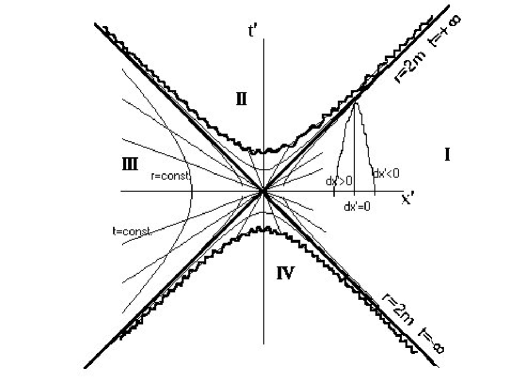
Figure 1: Kruskal diagram.

References

• [1] Luminet,J.P. (1998), astro-ph/9801252
• [2] Cooperstock,F. & Juvenicus,G. (1973) Nuovo Cim. 16B, 387
• [3] Mitra,A. (1999), astro-ph/9904162
• [4] Misner,C., Thorne,K. & Wheeler,J. (1973) Gravitation, Freeman, San Francisco
• [5] Cavalleri,G. & Spinelli,G. (1973) Let.Nuovo Cim. 6, 5
• [6] Janis,A. (1973) Phys.Rev.D 8, 2360
• [7] Cavalleri,G. & Spinelli,G. (1977) Phys.Rev.D 15, 3065
• [8] Janis,A. (1977) Phys.Rev.D 15, 3068