The Radial Structure of the Cygnus Loop Supernova Remnant
— Possible evidence of a cavity explosion —

Abstract

We observed the North-East (NE) Limb toward the center region of the Cygnus Loop with the ASCA Observatory. In our previous paper (Miyata et al. 1994), we analyzed the data obtained with the X-ray CCD cameras (SISs). We found a radial variation of electron temperature ($kT_{\rm e}$) and ionization timescale (log($\tau$)) whereas no variation could be found for the abundances of heavy elements. In this paper, we re-analyzed the same data set and new observations with the latest calibration files. Then we constructed the precise spatial variations of $kT_{\rm e}$, log($\tau$), and abundances of O, Ne, Mg, Si, and Fe over the field of view (FOV). We found a spatial variation not only in $kT_{\rm e}$ and in log($\tau$) but also in most of heavy elements. As described in Miyata et al. (1994), values of $kT_{\rm e}$ increase and those of log($\tau$) decrease toward the inner region. We found that the abundance of heavy elements increases toward the inner region. The radial profiles of O, Ne, and Fe show clear jump structures at a radius of 0.9 $R_{\rm s}$, where $R_{\rm s}$ is the shock radius. Outside of 0.9 $R_{\rm s}$, abundances of all elements are constant. On the contrary, inside of 0.9 $R_{\rm s}$, abundances of these elements are 20–30 % larger than those obtained outside of 0.9 $R_{\rm s}$. The radial profile of $kT_{\rm e}$ also shows the jump structure at 0.9 $R_{\rm s}$. This means that the hot and metal rich plasma fills the volume inside of 0.9 $R_{\rm s}$. We concluded that this jump structure was the possible evidence for the pre-existing cavity produced by the precursor. If the ejecta fills inside of 0.9 $R_{\rm s}$, the total mass of the ejecta was roughly 4$\hskip 1.42262ptM_{\odot}$. We then estimated the main-sequence mass to be roughly 15$\hskip 1.42262ptM_{\odot}$, which supports the massive star in origin of the Cygnus Loop supernova remnant and the existence of a pre-existing cavity.

1 Introduction

The X-ray emission of the shell-type supernova remnants (SNRs) is mainly due to the thermal emission from the shock heated plasma. The standard model of the dynamical evolution of SNRs shows that the reverse shock wave propagates into the ejected material and the fore shock wave expands into the ambient medium (McKee 1974). The shocked material is separated at the contact discontinuity between the ejecta and the interstellar medium (ISM). Many theoretical calculations have been performed to follow the dynamical evolution of SNRs (e.g. Mansfield & Salpeter 1974, Chevalier 1982).

Just after being engulfed by the blast wave, the shocked matter is accelerated up to 3/4 $V_{\rm s}$, where $V_{\rm s}$ is the shock velocity, due to the mass conservation. The kinetic energy of electron gas, 1/2 $m_{\rm e}$ (3/4$V_{\rm s}$)², is roughly 2000 times smaller than that of ion gas, 1/2 $m_{\rm i}$ (3/4$V_{\rm s}$)², where $m_{\rm e}$ and $m_{\rm i}$ are masses of electron and ion, respectively. Shklovskii (1962) proposed that the equipartition between the ion gas and the electron gas could be established only by Coulomb collisions. In this case, the timescale for the equipartition is longer than the age of SNRs (Itoh 1978). The model to consider the deviation from the thermal equilibrium is called a two-fluid model. On the other hand, McKee (1974) proposed that collisionless shocks with high Mach number could equilibrate $T_{\rm e}$ and $T_{\rm i}$ by plasma instabilities or turbulence (one-fluid model), where $T_{\rm e}$ and $T_{\rm i}$ are the temperatures of electron gas and ion gas, respectively.

The previous X-ray observations (Aschenbach 1985; Bleeker 1990) show that the $kT_{\rm e}$ of young SNRs indicates that the electron gas is heated up to several keV, which is much higher than that expected from the non-equipartition model. Bleeker (1990) suggested that $T_{\rm e}$ $\simeq$ $T_{\rm i}$ was not grossly in error. On the other hand, based on the analysis of the optical observations of Balmer-dominant SNRs, Smith et al. (1991) showed that the ratios of broad to narrow H$\alpha$ intensity corresponded to neither the one-fluid nor the two-fluid model. The results of plasma measurements near the Earth bow shock support the two-fluid model (Montgomery et al. 1970).

The Cygnus Loop is one of the best-studied SNRs in radio, infrared, optical, and X-ray wavelengths. Its high surface brightness and large apparent size make it an ideal object for the study of the various shock heating conditions and spatially-resolving spectroscopy in detail. Various optical observations of the Cygnus Loop support a cavity explosion model which was initially proposed by McCray & Snow (1979). Hester & Cox (1986) and Hester et al. (1994) investigated the optical emission as well as the X-ray emission at bright shell regions of the Cygnus Loop and concluded that the bright X-ray emission originated not from evaporative clouds but from locally high density regions, suggesting the presence of large clouds around the Cygnus Loop. Shull & Hippelein (1991) measured proper motions at 39 locations within the Cygnus Loop and found an asymmetric expansion of the shell. They also concluded the existence of a pre-existing cavity wall around the Cygnus Loop. This model is supported by observations of coronal iron line emission (Teske 1990) and by observations with IRAS (Braun & Strom 1986).

Charles et al. (1985) observed the western edge of the Cygnus Loop with the Einstein Observatory. They found that $kT_{\rm e}$ increased toward the center and that the emission measure was proportional to the inverse square of $kT_{\rm e}$. They concluded that the bright X-ray emission was due to cloud evaporation and suggested the presence of a pre-existing cavity wall. Miyata et al. (1998) found the mass of the progenitor star of the Cygnus Loop to be $\simeq$ 25$\hskip 1.42262ptM_{\odot}$. This result also supports the presence of the pre-existing cavity.

In this paper, we present the radial profile from the NE limb toward the central region. Miyata et al. (1994; hereafter MTPK) observed the NE portion of the Cygnus Loop with the ASCA Observatory. They obtained moderate resolution X-ray spectra with the X-ray CCD camera, SIS. They determined both $kT_{\rm e}$ and the abundances of heavy elements. They found no spatial variations of the abundances of heavy elements. Data set we used for the NE limb was that of the same as MTPK.

2 Observations and Data Corrections

The NE limb (reg-1) and the inner region (reg-2) of the Cygnus Loop were observed with ASCA for  $\sim$8 and  $\sim$10 ks on Apr. 20 and Dec. 17-18, 1993, respectively. The ASCA Observatory, the fourth Japanese X-ray satellite (Tanaka, Inoue, & Holt 1994), is equipped with four X-ray telescopes (XRT; Serlemitsos et al. 1995) that simultaneously feed four focal plane instruments. The data reported here were obtained from the two Solid-state Imaging Spectrometers (SIS0 and SIS1; Yamashita et al. 1997) which have a FOV of 22′$\times$ 22′ and an energy resolution of approximately 60 eV full width at half maximum below 1 keV. The telescopes have a point spread function with a half power diameter (HPD) of about 3′.

In this paper, we re-analyzed the SIS data obtained at the NE limb using the latest software and calibration files available at the time of this writing. We employed Ftools ver 3.5 and Xselect ver 1.3 to extract our data sets. We excluded all the data taken at elevation angles below 5^∘ from the night earth rim and 50^∘ (for SIS) from the day earth rim, a geomagnetic cutoff rigidity lower than 6 GeV c^-1, and the region of the South Atlantic Anomaly. After screening with above criteria, we manually removed the time region where we could see a sudden change in light curves of the corner pixels of X-ray events. Then, we removed the hot and flickering pixels and corrected CTI, DFE, and Echo effects (T. Dotani et al. 1995, ASCA Letter News 3, 25; T. Dotani et al. 1997, ASCA Letter News 5, 14) in our data sets by using sispi and faint commands with the calibration file of sisph2pi_290296.fits. We considered the time-dependent effects of CTI and Echo whereas MTPK did not. Since these effects could be corrected only for the Faint-mode data, we focused only on the Faint-mode data for the spectral analysis. The observing times of the Faint-mode data for reg-1 and reg-2 were $\sim$ 7.3 and $\sim$ 4.6 ks after screening the data. We subtracted a blank-sky spectrum (North Ecliptic Pole and Lynx field regions) as the background, since we estimated the contribution of the Galactic X-ray background to be negligibly small (Koyama et al. 1986). The count rates for reg-1 and reg-2 in our FOV were $\sim$ 13 and $\sim$ 6.8 c ${\rm s^{-1}}$ /SIS. We used xanadu ver 8.5 for the spectral analysis performed in this paper.

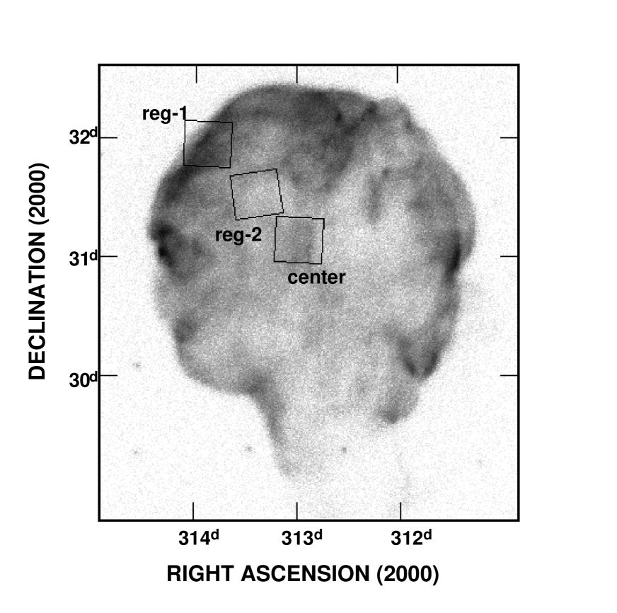
Figure 1: X-ray surface brightness map of the Cygnus Loop obtained by the ROSAT all-sky survey (Aschenbach 1994). The black squares show the FOVs of reg-1, reg-2, and the center portion as observed with the ASCA Observatory.

Figure 1 shows the location of our SIS FOVs superimposed on the X-ray surface brightness map of the Cygnus Loop (Aschenbach 1994) with black squares. The location of the observation by Miyata et al. (1998) is also shown as ‘center’ in this figure.

3 Spectral Analysis

Figure 2 shows the spatially integrated spectra both of reg-1 and of reg-2 after subtracting background. We clearly see K emission lines from O, Ne, Mg, Si, and S and L emission lines from Fe in reg-1. In reg-2, Si and S emission lines are strong whereas the other emission lines which appeared in reg-1 are not clearly seen. In the following fit procedures, we fixed the neutral H column to be $4\times 10^{20}\ {\rm cm}^{-2}$ (Inoue et al. 1979; Kahn et al. 1980).

3.1 Spectral Variation over the FOV

We investigated the spatial variations of the plasma structure over the FOV. We divided our FOV into 3′ squares each of which corresponds to the HPD of the XRT (Serlemitsos et al. 1995). Furthermore, we arranged the small squares such that each square was overlapping by 2′ with adjacent squares, resulting 400 squares for each region. Since the optical axes of SIS0 and SIS1 were different from each other, we employed the ascatool library to adjust the optical axes.

Then, we applied the single component non-equilibrium ionization (NEI) model coded by K. Masai (Masai 1984; Masai 1994) to each spectrum. Free parameters of the fitting were $kT_{\rm e}$, log($\tau$), abundances of O, Ne, Mg, Si, Fe, and Ni, and emission measure (EM [$\rm{\hskip 2.84526pt{cm}^{\scriptscriptstyle-6}}$ pc]). Values of reduced $\chi^{2}$ scattered from 1 to 2.

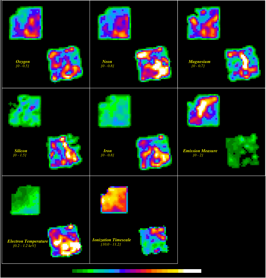
Figure 3: Spatial distribution of abundances of O, Ne, Mg, Si, and Fe and EM, $kT_{\rm e}$, and log($\tau$). Abundances, $kT_{\rm e}$, and EM are shown in cosmic abundance, in keV, and in ${\rm cm}^{-6}$pc, respectively. Each image was smoothed with a Gaussian function of FWHM=3^′.

Figure 3 shows the spatial variations of abundances of O, Ne, Mg, Si, and Fe relative to the cosmic abundance, EM, $kT_{\rm e}$, and log($\tau$). Filamentary-like structures are found in Si and Mg maps. However, we focused on the global structure of distribution of heavy elements. Abundances of heavy elements increase toward the inner region even in the cases of Si and Mg maps. Abundance variations can be found even inside reg-1. Except Si, abundances are smaller than the cosmic values. Obtained values of emission measure are anti-correlated with those of $kT_{\rm e}$ whereas they are well correlated with those of log($\tau$). These facts were already found in reg-1 by MTPK.

3.2 Radial Distribution of the Plasma Structure

As shown in figure 3, we found that there were structures in the radial direction rather than the azimuthal direction in the abundance maps as well as in other physical parameters. Therefore, we divided our FOV into 7 and 8 annular sectors for reg-1 and reg-2 to investigate the radial distribution of plasma structure as performed by MTPK. Each sector was separated by  $\sim$3′. The spectrum extracted from each region is shown in figures 4–5. All spectra have been background subtracted properly. We noticed that slopes in the energy range of $0.5-0.9$ keV generally change from (i) to (o) in reg-1. This indicated that values of $kT_{\rm e}$ decreased from the inner region to the outer region. We also noticed that the line intensity ratios of O VIII to O VII increased toward the center, suggesting higher $kT_{\rm e}$ or lower log($\tau$) at the inner region. In reg-2, Si emission line is generally stronger than that in reg-1. The continuum emission in reg-2 extends to higher energy than that in reg-1, suggesting higher $kT_{\rm e}$ in reg-2 compared with that in reg-1.

We again applied the single component Masai model to the 15 spectra. Free parameters are the same as those used in the previous section. Single component Masai model gave us reasonable fits to all regions. Best fit curves are shown in figures 4–5 by solid lines. The obtained $kT_{\rm e}$, log($\tau$), and EM are summarized in figure 6. We, here, assumed the shock radius, $R_{\rm s}$, to be 84′(Ku et al. 1984; hereafter KKPL).

3.2.1 $N_{\rm H}$ Uncertainties

Leahy et al. (1994) found that $N_{\rm H}$ was not uniform across the Cygnus Loop and increased from west-southwest to east-northeast. Based on their results, $N_{\rm H}$ changed from the center portion ($\approx 3.0\times 10^{20}$cm^-2) toward the eastern region ($\approx 5.0\times 10^{20}$cm^-2). The angular resolution of their observation is not high enough to compare with our data sets but there are no other results for $N_{\rm H}$ variations. Therefore, we fixed $N_{\rm H}$ to be 2.0$\times 10^{20}$ and 6.0$\times 10^{20}$ cm^-2 and fit the spectra. The obtained values for $kT_{\rm e}$, log($\tau$), and EM changed less than 5%, 1%, and 15%, respectively. Values of metal abundances changed less than 5%. All these changes were less than the statistical errors. Therefore, such variation in the $N_{\rm H}$ value does not affect our fitting results significantly.

3.2.2 Reg-1

In reg-1, we found that $kT_{\rm e}$ increased from the outer region (o) toward the inner region (i) whereas log($\tau$) decreased. Values of EM have a maximum just behind the shock front. The radial distribution of $kT_{\rm e}$ seen in figure 6 is consistent with those shown in figure 3. The gradient is qualitatively consistent with that expected from a model of simple blast wave propagating into a homogeneous medium.

These results are qualitatively similar to those obtained by MTPK whereas our results are systematically different from those of MTPK. Comparing with those of MTPK, our results show 20$-$30% higher values of $kT_{\rm e}$, resulting in lower EM. There are several reasons to account for discrepancies between our results and those by MTPK. One of the major reasons is that we use the Masai model whereas MTPK used the NEI model coded by J. Hughes (Hughes model; Hughes & Helfand 1985, Hughes & Singh 1993). There are differences in the atomic codes used in the Masai model (Kato model; Kato 1976) and those in the Hughes model (RS model; Raymond & Smith 1977). Another reason is that the calibration and understanding of the SIS as well as the XRT have been greatly improved since the writing of MTPK. We employed the latest calibration files, data processing software, and response matrices compared with those of MTPK as explained in section 2. Therefore, we believe that our current results are more reliable than those of MTPK.

Figure 7 shows the radial structures of the abundances of heavy elements relative to cosmic values. We find significant variations from (i) to (o) for O, Ne, Mg, and Fe. The radial profiles of all elements except Si show clear jump structure between (l) and (m) which is located at 0.9 $R_{\rm s}$. Outside of 0.9 $R_{\rm s}$, all profiles show constant values. On the contrary, interior of 0.9 $R_{\rm s}$, all profiles seem to show marginal increases toward the inner region.

We performed a statistical test on the radial distributions of metal abundances. We assumed that abundances of all elements were constant inside of $r_{1}$ ($0.75<r_{1}<1$) and outside of $r_{1}$ they were also constant but different values for all elements, where $r_{1}$ was a projected radius. We fitted the abundance distributions for all elements simultaneously as a function of $r_{1}$ based on this assumption. Fitting result is shown in figure 8. Apparently, the abundance distribution of heavy elements is not constant in reg-1. There is only one acceptable radius of $r_{1}\approx$ 0.9 $R_{\rm s}$ even at 99 % confidence level. Therefore, the presence of the jump structure in the radial distributions of heavy elements is statistically significant.

3.2.3 Reg-2

In reg-2, the obtained values of $kT_{\rm e}$ are much higher than those of reg-1 as shown in figure 6. We should note that $kT_{\rm e}$ values in the inner region of reg-2 are higher than those in the center portion of the Cygnus Loop (Miyata et al. 1998). On the contrary, values of log($\tau$) decrease toward the inner region.

For the radial distribution of heavy elements shown in figure 7, there are no common tendencies although scatter is large. The abundances of O and Ne at reg-2 are rather smaller than those in reg-1 whereas that of Mg is similar to that of reg-1. Those of Si and Fe increase from reg-1 toward reg-2.

4 Discussion

4.1 Radial Profiles of the Electron Gas

We first investigated radial profiles of physical parameters of reg-1 shown in figure 6. Our results reflect the projected profiles along the line of sight. The theoretical calculations usually describe unprojected profiles. Assuming the spherical symmetry, we calculate the projected profiles to compare with our results.

We use two kinds of coordinate systems. Both of them are centered on the explosion center (${\rm\alpha=20^{h}49^{m}15^{s}}$, ${\rm\delta=30^{\circ}51^{\prime}30^{\prime\prime}}$ (1950); KKPL). One is the observational system projected on the sky ($\boldmath r$). The other is unprojected system of the SNR ($\boldmath R$). In both systems, we use the coordinate by normalizing the current location of the shock front, $R_{\rm s}$.

4.1.1 $kT_{\rm e}$ profile

(i) Sedov model

As written in section 1, there are mainly two plausible models which account for the electron heating mechanism: a one-fluid model and a two-fluid model. Kahn (1975) developed an analytic method to describe the physical structures in adiabatic SNRs based on the one-fluid model. Cox & Franco (1981) described the two-fluid condition by using the approximation technique introduced by Itoh (1978) and derived an approximation formulae to describe thermal structures for adiabatic SNRs. For the two-fluid model, the evolution of $kT_{\rm e}$ depends on the explosion energy, $E_{51}$ (in units of $\rm{\hskip 2.84526pt{10}^{\scriptscriptstyle 51}}$ erg), the density of the ambient medium, $n_{0}$ (in unit of ${\rm cm^{-3}}$), and the age of the remnant, $t_{3}$ (in units of $\rm{\hskip 2.84526pt{10}^{\scriptscriptstyle 3}}$ yr). We assume $n_{0}$ to be $0.2\ {\rm cm}^{-3}$ (KKPL). $kT_{\rm e}$ just behind the shock front ($T_{\rm s}$) is roughly 0.3 keV as shown in figure 3. By using these parameters, we can determine $E_{51}$ and $t_{3}$ with the Sedov equations (Sedov 1959),

$$T_{\rm s} = 1.5\times 10^{10}\times\frac{E_{51}}{n_{0}}R_{\rm s}^{-3}$$ (1)

$$= 1.2\times 10^{8}\ \frac{E_{51}}{n_{0}}^{2/5}t_{3}^{-6/5}\ ,$$ (2)

to be 0.3 and 22, respectively. Applying these values, we calculate the thermal structure based on the two-fluid model. Figure 9 shows unprojected radial profiles of $kT_{\rm e}$($R$) based both on the one-fluid model and on the two-fluid model using the calculations by Cox & Franco (1981). As seen in this figure, we expect that $kT_{\rm e}$($R$) increases toward the center region in both cases. In the range of 0.8 $<R<$ 0.99, the equipartition between ion and electron has achieved even if we consider only Coulomb heating of electrons. Therefore, we expect that the radial profile of $kT_{\rm e}$($r$) is similar if we use either the one-fluid model or the two-fluid model. This figure shows the unprojected radial profile of $kT_{\rm e}$($R$) while our result (figure 6) shows the projected profile. We then calculate the projected radial profile based on these models.

For simplicity, we assume that $kT_{\rm e}$ is determined by the continuum emission through the spectral fitting procedure. We thus calculate the spectrum of the thermal bremsstrahlung emission integrated along the line of sight weighted by EM for one-fluid model and two-fluid model. We adopt the Kahn’s approximation for $n_{\rm e}$($R$). After calculating the projected spectra, we fit them with the single $kT_{\rm e}$ thermal bremsstrahlung, considering the effective area of SIS in the energy range of $0.4-4$ keV. Therefore, the projected radial profile of $kT_{\rm e}$($r$) is valid only for the results obtained with the SIS.

Figure 10 shows the projected radial profiles of $kT_{\rm e}$($r$). As we expected, the radial profiles of $kT_{\rm e}$($r$) are similar for both models. Based on either model, $kT_{\rm e}$($r$) linearly increases toward the center. In the range of $r>$ 0.75, $kT_{\rm e}$($r$) is approximately described as ($0.98-0.71\ r$) keV. Our results show higher $kT_{\rm e}$ at $r<$ 0.9 than those expected from both models. We then modify the unprojected models to reproduce our results.

(ii) Modified Two-Fluid Model

As shown in figure 7, the radial profiles of abundances of heavy elements have a discontinuity at $r\approx$ 0.9. We also see that the radial profile of $kT_{\rm e}$ as shown in figure 6, shows a jump structure at $r\approx$ 0.9. Therefore, we calculate the radial profile of $kT_{\rm e}$($r$) in the case that $kT_{\rm e}$($R$) has a discontinuity at $R$ = 0.9. In this calculation, we adopt the two-fluid model since there is little difference between one-fluid and two-fluid model as shown in figure 10. In the region of $R\geq$ 0.9, the radial profiles of $kT_{\rm e}$($R$) and $n_{\rm e}$($R$) are almost the same as those by the two-fluid model as described in section 4.1.1. For $R<$ 0.9, we introduce an extra parameter, $\gamma$, to characterize the jump condition at $R$ = 0.9 in the radial profiles of $kT_{\rm e}(R)$ and $n_{\rm e}$($R$). Here, we assumed that the value of $kT_{\rm e}$ was constant at $R<$ 0.9 and that it was $\gamma$ times higher than that of $kT_{\rm e}$ at $R$ = 0.9. For pressure equilibrium, the value of $n_{\rm e}(R<$ 0.9) was assumed to be $\gamma$ times lower than that of $n_{\rm e}$ at $R$ = 0.9. We call this model a modified two-fluid model. Figure 11 shows the radial profiles of $kT_{\rm e}$ and $n_{\rm e}$ for the modified two-fluid model by dashed lines as well as those for the two-fluid model shown by solid lines. Here, we assumed $\gamma$ to be 10. Values of $kT_{\rm e}$ and $n_{\rm e}$ were normalized to those at $R_{\rm s}$.

Based on this figure, we calculated the spectra at each unprojected radius, integrated them along the line of sight, and fitted them at each projected radius as the same way in section 4.1.1. Results are shown in figure 12.

As mentioned in section 4.1.1(i), values of $kT_{\rm e}$(r) based both on the one-fluid model and on the two-fluid model are lower than our results at $r<$ 0.9. For the modified two-fluid model, the calculated profile was in reasonable agreement with our data. Therefore, we preferred the modified two-fluid model rather than one-fluid or two-fluid models without jump structures. Considering the statistics of our data, $\gamma$ ranges between 5 and 15.

(iii) Radial Profiles from Reg-1 to Reg-2

We then applied the modified two-fluid model both for reg-1 and for reg-2. Figure 13 shows the radial profile of $kT_{\rm e}$ both for reg-1 and reg-2 as well as our calculations based on the one-fluid model, the two-fluid model, and the modified two-fluid model with $\gamma$=10. It is interesting to note that apparent values of $kT_{\rm e}$ based on the one-fluid model decrease toward the center at $r\leq$ 0.6. The expected $kT_{\rm e}$ at the inner region is much higher than that at the shell region based on the one-fluid model. Plasma with high $kT_{\rm e}$ ($\geq$ 10 keV) does not affect our data while that with several keV can increase the observed $kT_{\rm e}$ value. In this sense, plasma at $R\geq$ 0.5 can raise the observed $kT_{\rm e}$ only in the case that the emission measure is enough to contribute. As shown in figure 11, $n_{\rm e}$ at $R$=0.5 is $\simeq$ 1 % at $R$ = 1, resulting $\simeq$ 3 orders of magnitude lower in emission measure. Such a small fraction is negligible and the emission in the shell region is dominant in the calculation. For this reason, the calculated value of $kT_{\rm e}$ based on the one-fluid model decreases toward the center.

The value of $kT_{\rm e}$ at $R\leq$ 0.9 based on the modified two-fluid model is similar to that at $R\simeq$ 0.6 of the one-fluid model. However, in the case of the modified two-fluid model, the contribution from the hotter plasma becomes larger as one moves toward the inner region. Thus, $kT_{\rm e}$ based on the modified two-fluid model increases toward the center at $R\leq$0.6. Therefore, the modified two-fluid model with $\gamma$ of 5–15 reasonably agrees with our results. There are still some deviations from our calculation at reg-2. This is probably due to the simplicity of the model. More sophisticated model including some patchy structure or local inhomogeneities would improve the fit to our results.

Chevalier (1975a) initially pointed out an importance of the electron thermal conduction for young SNRs and also suggested its importance on the structure of the hot interior for evolved SNRs. Chevalier (1975b) constructed an evolutionary model including the electron thermal conduction based on the Mansfield & Salpeter model (1974). Silk (1977) also calculated the evolutional scenario including the electron thermal conduction. In both models, $kT_{\rm e}$ goes up suddenly just behind the shock front and stays constant value roughly at $R\leq$ 0.6. The electron density has a sharp peak just behind the shock front due to a shell formation, decreases from the shock front toward an inner region, and stays constant value at $R\leq$ 0.6. Chevalier’s model and Silk’s model are similar to our model except for the location of the jump structure. Our observational result shows much stronger X-ray flux at the shell region compared with their models. We suppose that the constant $kT_{\rm e}$ at the inner region is due to the electron thermal conduction.

4.1.2 Emission Measure

Next, we investigate the radial distribution of EM($r$) in the same way as that of $kT_{\rm e}$($r$). Figure 14 shows EM($r$) for the three cases. Dash-dot, solid, and dotted lines show EM($r$) based on the one-fluid, the two-fluid, and the modified two-fluid model, respectively.

For the radial profile of EM($r$), neither the one-fluid model nor the two-fluid model can reproduce our observational results inside of $R\simeq$ 0.9. On the contrary, the modified two-fluid model with $\gamma$ of 10 is in good agreement with our results. In this case, the electron density of the ambient medium is roughly 0.25 ${\rm cm}^{-3}$.

Taking into account the result of the radial profile of $kT_{\rm e}$, only the modified two-fluid model with $\gamma$ of 5–15 can reproduce the SIS results. The electron density of the inner region ($R\leq$ 0.9) can be calculated as $\simeq 8\times 10^{-3}{\rm cm}^{-3}$. This suggests that the hot tenuous plasma extends inside of $R\simeq$ 0.9.

4.2 Jump in Metal Abundance at 0.9$R_{\rm s}$

As shown in figure 7, there is a jump structure at $r\simeq 0.9$ in the radial distributions of heavy elements. Here, we discuss the possible causes to explain the jump structure.

4.2.1 Dust Sputtering ?

The Copernicus satellite has studied the depletion along the line of sight for various elements (see review for Spitzer & Jenkins 1976). The depletion of Fe compared with other elements like C, N, or O suggests that Fe and other missing gas-phase elements are bound to interstellar grains. After being engulfed by the shock wave, the dust grains containing metal are destroyed in the postshock region due to the nonthermal sputtering or due to grain-grain collisions (Seab & Shull 1983). Employing the experimental data by KenKnight & Wehner (1964) and an approximation formula by Almén & Bruce (1961), the timescale of the grain destruction, $t_{\rm s}$, is roughly estimated as,

$$t_{\rm s}\,\,\approx\,\,10^{5}\,\,\left(\frac{n_{\rm e}}{1{\rm cm}^{-3}}\right)^{-1}\,\,\left(\frac{T_{\rm e}}{10^{6}{\rm K}}\right)^{-1/2}\,\,\,\,{\rm yr}.$$ (3)

As dust grains are destroyed, heavy elements return to the gas phase. Dust grains at the center regions would be sputtered for a longer time than those at the shell, resulting the increase of abundances of heavy elements toward the center. This picture seems to qualitatively explain our results. However, as apparent in figure 7, the abundance of Ne increases toward the center. Since Ne is a rare gas, there is no observational results of the depletion of Ne. Therefore, it is difficult to explain the increase of abundances solely by the dust sputtering model.

We should note that the derived Ne abundance contains some ambiguity. Since emission lines from Ne overlap the energy range of Fe-L emission line blends, the abundance of Ne is partly affected by that of Fe. There are also uncertainties in the atomic code of Fe-L blends (e.g. Liedahl et al. 1995). In the future, we will be able to detect the Ne lines free from Fe-L blends to obtain the true Ne abundance using X-ray detectors with a good energy resolving power. To investigate the model of the dust sputtering in detail, we need observations with higher energy resolving power which can be realized in with the next Japanese X-ray satellite, Astro-E (Inoue 1997).

4.2.2 Contact Discontinuity ?

A more straightforward way to explain the increase of abundances would be with contributions of ejecta. Ejecta are considered to fill the region inside of the contact discontinuity. Based on Chevalier’s similarity solutions (1982), the location of the contact discontinuity ($R_{\rm c}$) is at 0.73–0.90 $R_{\rm s}$ depending on density profiles of the circumstellar matter and of the ejecta. Since the ejecta fill the region inside of the contact discontinuity, we expect an increase of the abundances of heavy elements in the vicinity of the contact discontinuity. Based on figure 7, we find a jump in the radial profiles of abundances at $r\approx$ 0.9. This value agrees well with the Chevalier’s calculations in the case that the blast wave propagates into a homogeneous medium. As Chevalier (1982b) pointed out, however, $R_{\rm c}$ becomes smaller as SNR evolves into the Sedov phase. During the Sedov phase, $R_{\rm c}$ is constant at $R\approx$ 0.75 (McKee 1974), which is too far in compared with our results. Therefore, it is not likely that the contact discontinuity exists at $R=0.9$.

4.2.3 Shell Formation ?

As described in section 4.1.1, both Chevalier’s model and Silk’s model suggested a sharp density peak just behind the shock front due to a shell formation. This would be a signature that a SNR has evolved into a radiative phase from an adiabatic Sedov phase. A width of the density peak is expected to be $\simeq$ 1 % of $R_{\rm s}$ which is an order of magnitude narrower than the enhancement in emission measure shown in figure 6. The expected $kT_{\rm e}$ is also much lower than that can be detected with the ASCA Observatory. Therefore, we ruled out that the density enhancement we observed was due to the shell formation.

We should note that the Cygnus Loop has already shifted into radiative phase at some places where we see optical filamentary structures (e.g. Raymond et al. 1988). Such filamentary structures trace radiative shock fronts. In our region, Hester et al. (1994) reported Balmer-dominated filaments due to nonradiative shocks as well as the H$\alpha$ filaments due to radiative shocks. Therefore, the radiative shock must have taken place in the NE region of the Cygnus Loop. However, we could not detect the density enhancement expected from the radiative shock due to the poor spatial resolving power. Future X-ray observations possessing much higher spatial resolution, like CXO and XMM, will clarify the shock structure in the NE region.

4.2.4 Pre-existing cavity ?

We found that the density of the bright shell region was much higher than that predicted by the model that the blast wave expanded into the homogeneous medium as mentioned in section 4.1. On the contrary, the density inside the shell was constant and quite low ($\simeq 8\times 10^{-3}{\rm cm}^{-3}$). These results are naturally interpreted with the hypothesis that the supernova (SN) which produced the Cygnus Loop occured within a pre-existing cavity wall (which was probably produced by the precursor). This hypothesis has been widely supported by infrared, optical, and X-ray observations. If a cavity exists before the SN explosion, the blast wave freely expands into the low density medium and suddenly hits the high density pre-existing cavity wall. The kinetic energy of the blast wave can be converted to thermal energy in the cavity and heat it up to emit X-rays. As the result, we expect that the metal abundances at the bright shell region reflect those of the ISM while the metal abundances at low density inner region reflect those of ejecta. This scenario fits our results both with respect to the radial profiles of $kT_{\rm e}$, EM, and the abundances of heavy elements.

4.3 Radial Profile in Metal Abundances

Miyata et al. (1998) found Si, S, and Fe rich plasma at the center portion of the Cygnus Loop. Such plasma was confined in a small region with the radius of $\simeq$ 9 ′. Our results suggest that Si and Fe may increase from (d) toward the center. Therefore, the major part of Si and Fe in ejecta might be confined well within the shell region.

If the ejecta fill only inside of 0.9 $R_{\rm s}$, the abundances in (m)–(o) reflect the ISM alone or the ISM contaminated by stellar wind from the progenitor star. Abundances of O and Ne at reg-2 are similar to those of reg-1 ($r<0.9$). These values are also similar to those obtained in the center portion of the Cygnus Loop (Miyata et al. 1988). Therefore, O and Ne in ejecta are distributed inside of $R_{\rm s}\leq 0.9$. Mg abundances in reg-2 are similar to those in (m)–(o), suggesting that the Mg in the ejecta is distributed possibly in $0.6\leq R_{\rm s}\leq 0.9$.

Mg abundance is distributed in the outer region compared with those of Si and Fe while O and Ne are uniformly distributed inside the shell. Based on the nucleosynthesis model in supernova calculated by Thielemann et al. (1996), heavy elements like Si, S, and Fe are produced in the inner region whereas light elements like O, Ne, and Mg are produced in the outer region of the progenitor star. Some fraction of Si and S are also synthesized in the outer region where O is the dominant element. This picture is in good agreement with our observational results. Therefore, our result is a possible evidence of the onion-skin structure in such an evolved SNR as the Cygnus Loop.

4.4 Progenitor Mass

Assuming $\gamma$ to be 10 in the modified two-fluid model, we can calculate the total mass contained inside $R$ = 0.9. The volume and the density inside $R$ = 0.9 ($\approx$ 16.6 pc) are $1.9\times 10^{4}{\rm pc}^{3}$ and $8\times 10^{-3}{\rm cm}^{-3}$, respectively. The total mass is roughly 4$\hskip 1.42262ptM_{\odot}$. If this is the progenitor mass, its main-sequence mass is estimated to be  $\sim$15$\hskip 1.42262ptM_{\odot}$(Nomoto, Hashimoto 1984). This strongly supports the massive star origin of the Cygnus Loop.

Charles et al. (1984) suggested the spectral type of the progenitor star of the Cygnus Loop to be later than B0 based on the radius of the cavity. Shull & Hippelein (1991) restricted the spectral type to be B stars rather than O stars. Since O stars tend to destroy almost anything around them due to the photoevaporation, they would not have left well-defined cavities or shells (Shull et al. 1985). Chevalier (1988) pointed out that 15$\hskip 1.42262ptM_{\odot}$ was a critical mass above which the circumstellar effects were large and below which they disappeared rapidly. This is due to the fact that the rate of emission of ionizing photons drops dramaticaly for stars later than B0 stars (Panagia 1973). Therefore, our estimate of 15$\hskip 1.42262ptM_{\odot}$ is consistent with the view of the pre-existing cavity.

In this case, the H-rich envelope mass of the progenitor star is roughly 10$\hskip 1.42262ptM_{\odot}$. If it is present outside of 0.9 $R_{\rm s}$, the width of the H-rich envelope is estimated to be  $\sim$0.3 pc, which is  $\sim$1′. This cannot be resolved with the ASCA Observatory. The XMM may reveal the plasma structure in the shell region in detail.

4.5 Mixing of the Ejecta with the ISM

We estimate the timescale for mixing of the ejecta with the shocked pre-existing cavity. The diffusion timescale, $\tau_{d}$, for the ejecta to mix with the surrounding gas is approximately

$$\tau_{d}=\frac{L^{2}}{D}\ \ ,$$ (4)

where $L$ is the typical size of the mixing region and $D$ is the diffusion coefficient. Taking into account Coulomb collisions solely, the mean free path of an ion, $\lambda$, is

$$\lambda = t_{\rm ee}\left(\frac{3kT_{\rm e}}{m_{\rm e}}\right)^{1/2}$$ (5)

$$= 0.29\ \left(\frac{T_{\rm e}}{10^{7}{\rm K}}\right)^{2}\left(\frac{n_{\rm e}}{1{\rm cm}^{-3}}\right)^{-1}\left(\frac{\ln\Lambda}{30}\right)^{-1}\ \ \ {\rm pc}\ \ \ ,$$ (6)

where $t_{\rm ee}$ is the relaxation timescale of the electron gas and $\ln\Lambda$ is the Coulomb logarithm. Then, $D$ is (Chevalier 1975)

$$D=\frac{1}{3}\lambda v=1.0\times\mbox{$\rm{\hskip 2.84526pt{10}^{\scriptscriptstyle 23}}$}\left(\frac{T_{\rm i}}{5\times 10^{6}{\rm K}}\right)^{5/2}\left(\frac{n_{\rm i}}{0.1{\rm cm}^{-3}}\right)^{-1}\left(\frac{Z}{10}\right)^{-2}\ \ \ {\rm cm}^{2}\ {\rm s}^{-1}\ \ \ ,$$ (7)

where $T_{\rm i}$ is the ion temperature and $n_{\rm i}$ is the ion density. $Z$ is the mean charge of heavy elements and roughly 10 in our case (Masai 1984). Since we find the boundary between the ejecta and the cavity as shown in figure 7, the transition region is smaller than the size of each annular sector which is equal to the PSF of the XRT. So we set $L$ to be $\leq$ 1 pc. The timescale for the mixing is

$$\tau_{d}=3.0\times 10^{6}\left(\frac{L}{1~{}{\rm pc}}\right)^{2}\left(\frac{T_{\rm i}}{5\times 10^{6}{\rm K}}\right)^{-5/2}\left(\frac{n_{\rm i}}{0.1{\rm cm}^{-3}}\right)\left(\frac{Z}{10}\right)^{2}\ \ \ {\rm yr}\ \ \ .$$ (8)

As mentioned by Chevalier (1975), this estimate may be shortened by the turbulent diffusion whereas this may be lengthened by the work of the magnetic field. However, these effects have not yet been established. The timescale shown above is a first approximation for the mixing of the ejecta in the shocked pre-existing cavity. Apparently, this timescale is much longer than the age of the Cygnus Loop. Therefore, the ejecta will not mix with the pre-existing cavity for next $10^{6}$ yr.

Figure 2: Spatially integrated spectra both at reg-1 and reg-2. Line identifications are also shown.

Figure 4: Best fit curves of the Masai model in reg-1

Figure 5: Same as figure 4 but for reg-2

Figure 6: Radial profiles of $kT_{\rm e}$, log($\tau$), and EM. Horizontal axis shows the angular distance from the center normalized by the shock radius. Errors are at 90% confidence level.

Figure 7: Same as figure 6 but for abundances of heavy elements relative to cosmic values.

Figure 8: $\chi^{2}$ distributions for all elements fitted with the step function. Horizontal solid line shows 90 % confidence level and dotted line shows 99 % confidence level.

Figure 9: Unprojected radial profiles of $kT_{\rm e}$ based on the one-fluid and the two-fluid models. Parameters to be used for the two-fluid model are $E_{51}$ = 0.3, $t_{3}$ = 22, and $n_{0}$ = 0.2.

Figure 10: Projected radial profiles of $kT_{\rm e}$. Our results are shown by stars. Model calculations based on the one-fluid and the two-fluid models are shown by dotted and solid lines, respectively.

Figure 11: Unprojected radial profiles of $kT_{\rm e}$ (upper pannel) and $n_{\rm e}$ (lower pannel), normalized by the values just behind the shock front. Solid lines and dashed lines show the radial profiles for the two-fluid model the modified two-fluid model, respectively. See text for details.

Figure 12: Projected radial profiles of $kT_{\rm e}$. Solid and dashed lines are calculated based on the two-fluid model and the modified two-fluid model, respectively. See text for details.

Figure 13: Same as figure 12, but used data sets both reg-1 and reg-2.

Figure 14: Radial profiles of EM for various models. Dash-dot, solid, and dotted curves are calculated based on the one-fluid model, the two-fluid model, and the modified two-fluid model.

References

- (1) Allen, C.W. 1973, Astrophysical Quantities 3rd ed. (The Athlone Press), 30
- (2) Almén, O., & Bruce, G. 1961, Nucl.Instr.Meth, 11, 257
- (3) Aschenbach, B. 1985, Space.Sci.Rev., 40, 447
- (4) Aschenbach, B. 1994, in New Horizon of X-ray Astronomy, ed. F. Makino & T. Ohashi (Universal Academy Press inc.), 103
- (5) Bleeker, J.A.M. 1990, Adv.Space Res., 10, (2)143
- (6) Braun, R. & Strom, R.G. 1986, A&A, 164, 208
- (7) Charles, P.A., Kahn, S.M. & McKee, C.F. 1985, ApJ, 295, 456
- (8) Chevalier, R.A. 1975a, ApJ, 198, 355
- (9) Chevalier, R.A. 1975b, ApJ, 200, 698
- (10) Chevalier, R.A. 1982, ApJ, 258, 790
- (11) Chevalier, R.A. 1982b, ApJ, 259, L85
- (12) Chevalier, R.A. 1985, in Hot Thin Plasma in Astrophysics, ed. R. Pallavicini (Kluwer Academic Publishers), p213
- (13) Cox,D.P. & Franco, J. 1981, ApJ, 251, 687
- (14) Gorenstein, P. et al. 1974, ApJ, 192, 661
- (15) Hester, J.J. & Cox, D.P. 1986, ApJ, 300, 675
- (16) Hester, J.J., Raymond, J.C., & Blair, W.P. 1994, ApJ, 420, 721
- (17) Hughes J.P., & Helfand D.J. 1985, ApJ, 291, 544
- (18) Hughes J.P., & Singh K.P. 1994, ApJ, 422, 126
- (19) Inoue, H., Koyama, K., Matsuoka, M., Ohashi, T., Tanaka, Y., & Tsunemi, H. 1979, in X-Ray Astronomy, ed. W.A. Baity & L.E. Peterson (Pergamon Press, Oxford), 309
- (20) Inoue, H. 1997, Proc. Leicester X-Ray Astronomy Group Special Report XRA97/02, p161
- (21) Itoh, H. 1978, PASJ, 30, 489; Erattum, 31, 429
- (22) Kahn, F.D. 1975, in 14th Int. Cosmic Ray Conf. (Munich), 11, 3566
- (23) Kahn, S.M., Charles, P.A., Bowyer, S., & Blissett, R.J. 1980, ApJ, 242, L19
- (24) Kato, T. 1976, ApJS, 30, 397
- (25) KenKnight, C.E., & Wehner, G.K. 1964, J.Applied Phys., 35, 419
- (26) Ku, W.H.-M., Kahn, S.M., Pisarski, R., & Long, K.S. 1984, ApJ, 278, 615 (KKPL)
- (27) Leahy, D.A., Fink, R. & Nousek, J. 1990, ApJ, 363, 547
- (28) Liedahl, D.A., Osterheld, A.L., & Goldstein, W.H. 1995, ApJ, 438, L115
- (29) Mansfield, V.N., & Salpeter, E.E. 1974, ApJ, 190, 305
- (30) Masai, K. 1984, Astrophys. Space Sci., 98, 367
- (31) Masai, K. 1994, Ap.J., 437, 770
- (32) McCray R., Snow T.P.Jr. 1979, ARA&A 17, 213
- (33) McKee, C.F., 1974, ApJ, 188, 335
- (34) Miyata, E., Tsunemi, H., Pisarski, R., & Kissel, S.E. 1994, PASJL, 46, L101 (MTPK)
- (35) Miyata, E., Tsunemi, H., Kohmura, T., Suzuki, S. & Kumagai, S. 1998, PASJ, 50, 2
- (36) Montgomery, M.D. et al. 1970, J.Geoph.Res., 75, 1217
- (37) Nomoto, K., Thielemann, F.-K., & Yokoi, K. 1984, ApJ, 286, 644
- (38) Nomoto, K., Hashimoto, M. 1988, Phys.Rep. 163, 13
- (39) Panagia, N. 1973, AJ, 307, 619
- (40) Raymond, J.C., & Smith, B.W. 1977, ApJS, 35, 419
- (41) Raymond, J.C., Hester, J.J., Cox, D., Blair, W.P., Fesen, R.A., & Gull, T.R. 1988, ApJ, 324, 869
- (42) Sedov, L.I. 1959, Similarity and Dimensional Methods in Mechanics, 10th ed. (New York: Academic Press)
- (43) Serlemitsos, P.J., Jalota, L., Soong, Y., Kunieda, H., Tawara, Y., Tsusaka, Y., Suzuki, H., Sakima, Y. et al. 1995, PASJ, 47, 105
- (44) Shull, P.Jr., Dyson, J.E., Kahn, F.D., & West, K.A. 1985, MNRAS, 212, 799
- (45) Shull, P.Jr. & Hippelein, H. 1991, ApJ, 383, 714
- (46) Shklovskii, I.S. 1962, Sov.Astron., 6, 162
- (47) Silk, J. 1977, ApJ, 215, 226
- (48) Smith, R.C. et al. 1991, ApJ, 375, 652
- (49) Tanaka, Y., Inoue, H., & Holt, S.S. 1994, PASJL, 46, L37
- (50) Teske, R.G. 1990, ApJ, 365, 256
- (51) Thielemann, F.-K., Nomoto, K., & Hashimoto, M. 1996, ApJ, 460, 408
- (52) Yamashita, A. Dotani, T., Bautz, M.W., Crew, G., Ezuka, H., Gendreau, K., Kotani, T., Mitsuda, K., Otani, C., Rasmussen, A., Ricker, G., & H. Tsunemi, 1997, IEEE Trans. NS, 44, 847