Cosmological Implications of the Fundamental Relations of X-ray Clusters

Abstract

Based on the two-parameter family nature of X-ray clusters of galaxies obtained in a separate paper, we discuss the formation history of clusters and cosmological parameters of the universe. Utilizing the spherical collapse model of cluster formation, and assuming that the cluster X-ray core radius is proportional to the virial radius at the time of the cluster collapse, the observed relations among the density, radius, and temperature of clusters imply that cluster formation occurs in a wide range of redshift. The observed relations favor the low-density universe. Moreover, we find that the model of $n\sim-1$ is preferable.

1 Introduction

Galaxy clusters are the largest virialized objects in the universe and provide useful cosmological probes, since several properties of clusters are strongly dependent on the cosmological parameters. For example, the statistics of X-ray clusters can serve as an excellent probe of cosmology. The abundance of clusters and its redshift evolution can be used to determine the cosmological density parameter, $\Omega_{0}$, and the rms amplitude of density fluctuations on the fiducial scale $8h^{-1}$ Mpc, $\sigma_{8}$ (e.g. White, Efstathiou, & Frenk 1993 ; Eke, Cole, & Frenk 1996 ; Viana & Liddle 1996 ; Bahcall, Fan, & Cen 1997 ; Fan, Bahcall, & Cen 1997). Moreover, temperature and luminosity function of X-ray clusters is also used for a cosmological probe. Taking account of the difference between cluster formation redshift and observed redshift, Kitayama & Suto (1996) computed a temperature and luminosity function semi-analytically; comparing the predicted temperature ($T$) and luminosity ($L_{\rm X}$) function with the observed ones, they conclude that $\Omega_{0}\sim 0.2-0.5$ and $h\sim 0.7$. However, one tenacious problem in such investigations is the discrepancy of $L_{\rm X}-T$ relation between observations and simple theoretical prediction. This relation should also be an important probe of the formation history and cosmology.

In a separate paper (Fujita & Takahara 1999; hereafter Paper I), we have shown that the clusters of galaxies populate a planar distribution in the global parameter space $(\log\rho_{0},\log R,\log T)$, where $\rho_{0}$ is the central gas density, and $R$ is the core radius of clusters of galaxies. This ’fundamental plane’ can be described as

$$X=\rho_{0}^{0.47}R^{0.65}T^{-0.60}=constant\>.$$ (1)

We thus find that clusters of galaxies form a two-parameter family. The minor and major axes of the distribution are respectively given by

$$Y=\rho_{0}^{0.39}R^{0.46}T^{0.80}\>,$$ (2)

$$Z=\rho_{0}^{0.79}R^{-0.61}T^{-0.039}\>.$$ (3)

The scatters of observational data in the directions of $Y$ and $Z$ are $\Delta\log Y=0.2$ and $\Delta\log Z=0.5$, respectively (Paper I). The major axis of this ’fundamental band’ ($Z$) is nearly parallel to the $\log R-\log\rho_{0}$ plane, and the minor axis ($Y$) describes the $L_{\rm X}-T$ relation.

In this Letter, we discuss cosmological implications of the relations we found in Paper I, paying a particular attention to the two-parameter family nature of X-ray clusters and to the difference between cluster formation redshift and observed redshift. In §2, we use spherical collapse model to predict the formation history of clusters of galaxies, and in §3, we predict the observable distribution of X-ray clusters.

2 Formation History of Clusters of Galaxies

In order to explain the observed relations between the density, radius, and temperature of clusters of galaxies, we predict them for a flat and an open universe theoretically with the spherical collapse model (Tomita 1969; Gunn & Gott 1972). For simplicity, we do not treat vacuum dominated model in this paper. For a given initial density contrast, the spherical collapse model predicts the time at which a uniform spherical overdense region, which contains mass of $M_{\rm vir}$, gravitationally collapses. Thus, if we specify cosmological parameters, we can obtain the collapse or formation redshifts of clusters. Moreover, the model predicts the average density of the collapsed region $\rho_{\rm vir}$.

In Paper I, we showed that the observed fundamental band are described by the two independent parameters $M_{\rm vir}$ and $\rho_{\rm vir}$. In particular, the variation of $\rho_{\rm vir}$ is basically identified with the scatter of $Z$. Since the spherical collapse model treats $\rho_{\rm vir}$ and $M_{\rm vir}$ as two independent variables, it can be directly compared with the observed fundamental band, as long as we assume that the core radius and the mass of core region are respectively a fixed fraction of the virial radius and that of the virial mass at the collapse redshift, as is adopted in this paper. Although the model may be too simple to discuss cosmological parameters quantitatively, it can plainly distinguish the relations between the density, radius, and temperature in a low-density universe from those in a flat universe, as shown below.

For the spherical model, the virial density of a cluster is $\Delta_{c}$ times the critical density of a universe at the redshift when the cluster collapsed ($z_{\rm coll}$). It is given by

$$\rho_{\rm vir}=\Delta_{c}\rho_{\rm crit}(z_{\rm coll})=\Delta_{c}\rho_{\rm crit,0}E(z_{\rm coll})^{2}=\Delta_{c}\frac{\Omega_{0}\rho_{\rm crit,0}(1+z_{\rm coll})^{3}}{\Omega(z_{\rm coll})}\>,$$ (4)

where $\Omega(z)$ is the cosmological density parameter, and $E(z)^{2}=\Omega_{0}(1+z)^{3}/\Omega(z)$. The index 0 refers to the values at $z=0$. Note that the redshift-dependent Hubble constant can be written as $H(z)=100hE(z)\rm\;km\;s^{-1}\;Mpc^{-1}$. We fix $h$ at 0.5. In practice, we use the fitting formula of Bryan & Norman (1998) for the virial density:

$$\Delta_{c}=18\pi^{2}+60x-32x^{2}\;,$$ (5)

where $x=\Omega(z_{\rm coll})-1$.

It is convenient to relate the collapse time in the spherical model with the density contrast calculated by the linear theory. We define the critical density contrast $\delta_{c}$ that is the value, extrapolated to the present time ($t=t_{0}$) using linear theory, of the overdensity which collapses at $t=t_{\rm coll}$ in the exact spherical model. It is given by

$$\delta_{c}(t_{\rm coll}) = \frac{3}{2}D(t_{0})\left[1+\left(\frac{t_{\Omega}}{t_{\rm coll}}\right)^{2/3}\right]\;\;\;\;(\Omega_{0}<1)$$ (6)

$$= \frac{3(12\pi)^{2/3}}{20}\left(\frac{t_{0}}{t_{\rm coll}}\right)^{2/3}\;\;\;\;(\Omega_{0}=1)$$ (7)

(Lacey & Cole 1993), where $D(t)$ is the linear growth factor given by equation (A13) of Lacey & Cole (1993) and $t_{\Omega}=\pi H_{0}^{-1}\Omega_{0}(1-\Omega_{0})^{-3/2}$.

For a power-law initial fluctuation spectrum $P\propto k^{n}$, the rms amplitude of the linear mass fluctuations in a sphere containing an average mass $M$ at a given time is $\delta\propto M^{-(n+3)/6}$. Thus, the virial mass of clusters which collapse at $t_{\rm coll}$ is related to that at $t_{0}$ as

$$M_{\rm vir}(t_{\rm coll})=M_{\rm vir}(t_{0})\left[\frac{\delta_{c}(t_{\rm coll})}{\delta_{c}(t_{0})}\right]^{-6/(n+3)}\;.$$ (8)

Here, $M_{\rm vir}(t_{0})$ is regarded as a variable because actual amplitude of initial fluctuations has a distribution. We relate $t=t_{\rm coll}$ to the collapse or formation redshift $z_{\rm coll}$, which depends on cosmological parameters. Thus, $M_{\rm vir}$ is a function of $z_{\rm coll}$ as well as $M_{\rm vir}(t_{0})$. This means that for a given mass scale $M_{\rm vir}$, the amplitude takes a range of value, and thus spheres containing a mass of $M_{\rm vir}$ collapse at a range of redshift. In the following, the slope of the spectrum is fixed at $n=-1$, unless otherwise mentioned. It is typical in the scenario of standard cold dark matter for a cluster mass range.

The virial radius and temperature of a cluster are then calculated by

$$r_{\rm vir}=\left(\frac{3M_{\rm vir}}{4\pi\rho_{\rm vir}}\right)^{1/3}\>,$$ (9)

$$T_{\rm vir}=\frac{\mu m_{\rm H}}{3k_{\rm B}}\frac{GM_{\rm vir}}{r_{\rm vir}}\>,$$ (10)

where $\mu(=0.6)$ is the mean molecular weight, $m_{\rm H}$ is the hydrogen mass, $k_{\rm B}$ is the Boltzmann constant, and $G$ is the gravitational constant.

3 Results and Discussion

Since equations (4) and (8) show that $\rho_{\rm vir}$ and $M_{\rm vir}$ are the functions of $z_{\rm coll}$ for a given $M_{\rm vir}(t_{0})$, the virial radius $r_{\rm vir}$ and temperature $T_{\rm vir}$ are also the functions of $z_{\rm coll}$ for a given $M_{\rm vir}(t_{0})$ (equations [9] and [10]). Thus, by eliminating $z_{\rm coll}$, the relations among them can be obtained. Since observational values reflect mainly the structures of core region while the theory predicts average values within the virialized region, we must specify the relation between the observed values $(\rho_{0},R,T)$ and theoretically predicted values $(\rho_{\rm vir},R_{\rm vir},T_{\rm vir})$. Since we assume that mass distribution of clusters is similar, $r_{\rm vir}\propto R$ and $T_{\rm vir}=T$, emphasizing that $r_{\rm vir}$ is the virial radius when the cluster collapsed (see Salvador-Solé, Solanes, & Manrique 1998). In this case, the typical gas density of clusters has the relation $\rho_{0}\propto f\rho_{\rm vir}$, where $f$ is the baryon fraction of the cluster. Since it is difficult to predict $f$ theoretically, we assume $f\propto M_{\rm vir}^{0.4}$, which is consistent with the observations and corresponds to $X\sim constant$ (Paper I). For definiteness, we choose

$$f=0.25\left(\frac{M_{\rm vir}}{10^{15}\rm\;M_{\sun}}\right)^{0.4}\>.$$ (11)

Figure 1 shows the predicted relations between $f\rho_{\rm vir}$, $r_{\rm vir}$, and $T_{\rm vir}$ for $\Omega_{0}=0.2$ and $1$. Since we are interested only in the slope and extent of the relations, we do not specify $M_{\rm vir}(t_{0})$ exactly. Moreover, since $M_{\rm vir}(t_{0})$ has a distribution, we calculate for $M_{\rm vir}(t_{0})=10^{16}\rm\;M_{\sun}$ and $5\times 10^{14}\rm\;M_{\sun}$. The lines in Figure 1 correspond to the major axis of the fundamental band or $Z$ because they are the one-parameter family of $\rho_{\rm vir}$. The width of the distribution of $M_{\rm vir}(t_{0})$ represents the width of the band or $Y$. The observational data of clusters are expected to lie along these lines according to their formation period. However, when $\Omega_{0}=1$, most of the observed clusters collapsed at $z\sim 0$ because clusters continue growing even at $z=0$ (Peebles 1980). Thus, the cluster data are expected to be distributed along the part of the lines close to the point of $z_{\rm coll}=0$ (segment ab). In fact, Monte Carlo simulation done by Lacey & Cole (1993) shows that if $\Omega_{0}=1$, most of present clusters ($M_{\rm vir}\sim 10^{15}\rm\>M_{\sun}$) should have formed in the range of $z_{\rm coll}<0.5$ (parallelogram abcd). When $\Omega_{0}=0.2$, the growing rate of clusters decreases and cluster formation gradually ceases at $z\lesssim 1/\Omega_{0}-1$ (Peebles 1980). Thus, cluster data are expected to be distributed between the point of $z_{\rm coll}=0$ and $z_{\rm coll}=1/\Omega_{0}-1$ and should have a two-dimensional distribution (parallelogram ABCD).

The observational data are also plotted in Figure 1. The data are the same as those used in Paper I. For definiteness, we choose $r_{\rm vir}=8R$ and $f\rho_{\rm vir}=0.06\rho_{0}$. The figure shows that the model of $\Omega_{0}=0.2$ is generally consistent with the observations. The slopes of lines both in the model of $\Omega_{0}=0.2$ and $\Omega_{0}=1$ seem to be consistent with the data, although the model of $\Omega_{0}=0.2$ is preferable. However, the model of $\Omega_{0}=1$ is in conflict with the extent of the distribution because this model predicts that the data of clusters should be located only around the point of $z_{\rm coll}=0$ in Figure 1.

Finally, we comment on the case of $n=-2$, which is suggested by the analysis based on the assumption that clusters have just formed when they are observed (e.g. Markevitch 1998). Figure 2 is the same as Figure 1b, but for $n=-2$. The theoretical predictions are inconsistent with the observational results, because the theory predicts rapid evolution of temperatures; there should be few clusters with high-temperature and small core radius.

The results of this Letter suggest $\Omega_{0}<1$, and that the clusters of galaxies existing at $z\sim 0$ include those formed at various redshifts. We also show that the model of $n\sim-1$ is favorable. Importantly, the location of a cluster in these figures tells us its formation redshift. In order to derive the cosmological parameters more quantitatively, we should consider merging history of clusters and predict the mass function of clusters for each $z$.

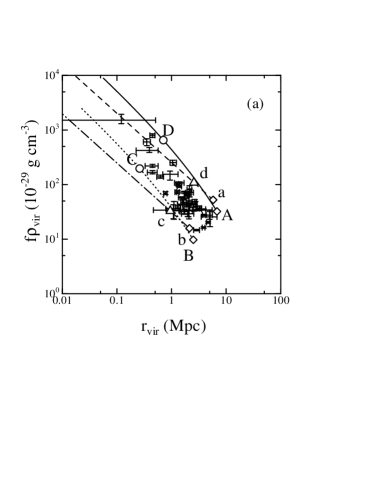
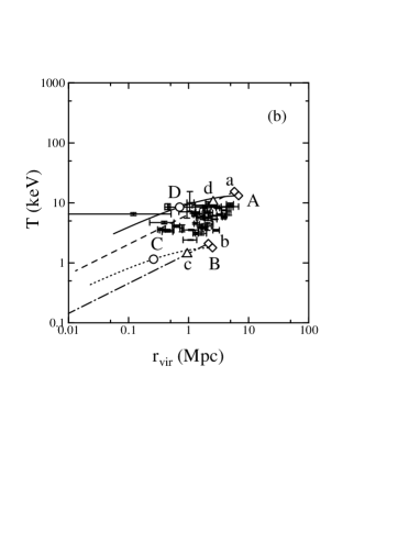
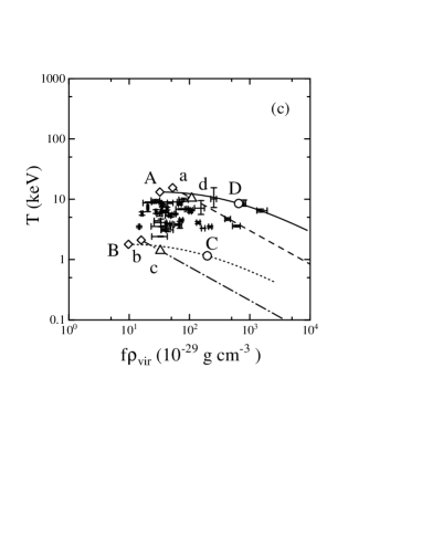
Figure 1: Theoretical predictions. (a) Radius–density relation (b) radius–temperature relation (c) density–temperature relation. Solid line: $\Omega_{0}=0.2$ and $M_{\rm vir}(t_{0})=10^{16}\rm M_{\sun}$. Dotted line: $\Omega_{0}=0.2$ and $M_{\rm vir}(t_{0})=5\times 10^{14}\rm M_{\sun}$. Dashed line: $\Omega_{0}=1.0$ and $M_{\rm vir}(t_{0})=10^{16}\rm M_{\sun}$. Dash-dotted line: $\Omega_{0}=1.0$ and $M_{\rm vir}(t_{0})=5\times 10^{14}\rm M_{\sun}$. The open diamonds (A, B, a, and b), circles (C and D), and triangles (c and d) correspond to $z_{\rm coll}=0$, $z_{\rm col}=1/\Omega_{0}-1$, and $z_{\rm col}=0.5$, respectively. The observational data ($\rho_{0}$, $R$, and $T$) are overlaid being shifted moderately in the directions of $\rho_{0}$ and $R$ ($\rho_{\rm vir}=0.06\rho_{0}$ and $r_{\rm vir}=8R$).

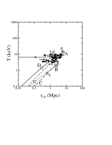
Figure 2: The same as Figure 1b, but for $n=-2$.

References

- (1) Bahcall, N. A., Fan, X., & Cen, R. 1997, ApJ, 485, L53
- (2)
- (3) Bryan, C. L., & Norman, M. L. 1998, ApJ, 495, 80
- (4)
- (5) Eke, V. R., Cole, S., & Frenk, C. S. 1996, MNRAS, 282, 263
- (6)
- (7) Fan, X., Bahcall, N. A., & Cen, R. 1997, ApJ, 490, L123
- (8)
- (9) Fujita, Y., & Takahara, F. 1999 (Paper I), ApJ Letters, in press (astro-ph/9905082)
- (10)
- (11) Gunn, J. E., & Gott, J. R. 1972, ApJ, 176, 1
- (12)
- (13) Kitayama, T., & Suto, Y. 1996, ApJ, 469, 480
- (14)
- (15) Lacey, C., & Cole, S. 1993, MNRAS, 262, 627
- (16)
- (17) Markevitch, M. 1998, ApJ, 504, 27
- (18)
- (19) Peebles, P. J. E. 1980, in The Large-Scale Structure of the Universe
- (20)
- (21) Salvador-Solé, E., Solanes, J. M., & Manrique, A. 1998, ApJ, 499, 542
- (22)
- (23) Tomita, K. 1969, Prog. Thor. Phys., 42, 9
- (24)
- (25) White, S. D. M., Efstathiou, G., & Frenk, C. S. 1993, MNRAS, 262, 1023
- (26)
- (27) Viana, P. T. P., & Liddle, A. R. 1996, MNRAS, 281, 323
- (28)