The Impact of the Massive Young Star GL 2591 on its Circumstellar Material: Temperature, Density and Velocity Structure

Abstract

The temperature, density and kinematics of the gas and dust surrounding the luminous ($2\times 10^{4}$ L_⊙) young stellar object GL 2591 are investigated on scales as small as $\sim 100$ AU, probed by $4.7$ $\mu$m absorption spectroscopy, to over $60,000$ AU, probed by single–dish submillimeter spectroscopy. These two scales are connected by interferometric $86-115$ and $226$ GHz images of size $30,000$ AU and resolution $2000$ AU in continuum and molecular lines. The data are used to constrain the physical structure of the envelope and investigate the influence of the young star on its immediate surroundings.

The infrared spectra at $\lambda/\Delta\lambda\approx 40,000$ indicate an LSR velocity of the ¹³CO rovibrational lines of $-5.7\pm 1.0$ km s^-1, consistent with the velocity of the rotational lines of CO. In infrared absorption, the ¹²CO lines show wings out to much higher velocities, $\approx-200$ km s^-1, than are seen in the rotational emission lines, which have a total width of $\approx 75$ km s^-1. This difference suggests that the outflow seen in rotational lines consists of envelope gas entrained by the ionized jet seen in Br$\gamma$ and [S II] emission. The outflowing gas is warm, $T>100$ K, since it is brighter in CO $J=6\to 5$ than in lower-$J$ CO transitions.

The dust temperature due to heating by the young star has been calculated self-consistently as a function of radius for a power-law density distribution $n=n_{0}r^{-\alpha}$, with $\alpha=1-2$. The temperature is enhanced over the optically thin relation $(T\sim r^{-0.4})$ inside a radius of $2000$ AU, and reaches $120$ K at $r{{}_{<}\atop{{}^{\sim}}}1500$ AU from the star, at which point ice mantles should have evaporated. The corresponding dust emission can match the observed $\lambda\geq 50$ $\mu$m continuum spectrum for a wide range of dust optical properties and values of $\alpha$. However, consistency with the C¹⁷O line emission requires a large dust opacity in the submillimeter, providing evidence for grain coagulation. The $10-20$ $\mu$m emission is better matched using bare grains than using ice-coated grains, consistent with evaporation of the ice mantles in the warm inner part of the envelope. Throughout the envelope, the gas kinetic temperature as measured by H₂CO line ratios closely follows the dust temperature.

The values of $\alpha$ and $n_{0}$ have been constrained by modelling emission lines of CS, HCN and HCO⁺ over a large range of critical densities. The best fit is obtained for $\alpha=1.25\pm 0.25$ and $n_{0}=(3.5\pm 1)\times 10^{4}$ cm^-3 at $r=30,000$ AU, yielding an envelope mass of $(42\pm 10)$ M_⊙ inside that radius. The derived value of $\alpha$ suggests that part of the envelope is in free-fall collapse onto the star. Abundances in the extended envelope are $5\times 10^{-9}$ for CS, $2\times 10^{-9}$ for H₂CO, $2\times 10^{-8}$ for HCN and $1\times 10^{-8}$ for HCO⁺. The strong near-infrared continuum emission, the Br$\gamma$ line flux and our analysis of the emission line profiles suggest small deviations from spherical symmetry, likely an evacuated outflow cavity directed nearly along the line of sight. The $A_{V}\approx 30$ towards the central star is a factor of 3 lower than in the best-fit spherical model.

Compared to this envelope model, the OVRO continuum data show excess thermal emission, probably from dust. The dust may reside in an optically thick, compact structure, with diameter ${{}_{<}\atop{{}^{\sim}}}30$ AU and temperature ${{}_{>}\atop{{}^{\sim}}}1000$ K, or the density gradient may steepen inside $1000$ AU. In contrast, the HCN line emission seen by OVRO can be satisfactorily modelled as the innermost part of the power law envelope, with no increase in HCN abundance on scales where the ice mantles should have been evaporated. The region of hot, dense gas and enhanced HCN abundance ($\sim 10^{-6}$) observed with the Infrared Space Observatory therefore cannot be accommodated as an extension of the power-law envelope. Instead, it appears to be a compact region ($r<175$ AU, where $T>300$ K) where high-temperature reactions are affecting abundances.

1 Introduction

The dust and molecular gas around low-mass young stellar objects (YSOs) is observed to consist of a disk of typical size $10^{2}$ AU, and a spherical power law envelope extending out to $r{{}_{>}\atop{{}^{\sim}}}10^{4}$ AU (0.05 pc). Perpendicular to the disk, a bipolar molecular outflow is often seen, reaching velocities up to $\sim 100$ km s^-1 (see reviews by Shu 1997, Blake 1997). Much less is known about the physical structure around high-mass YSOs (Churchwell 1993, 1999). Because the formation of massive stars occurs over much shorter time scales and involves much higher luminosities, differences in the structure of the circumstellar environment may be expected. Submillimeter continuum observations have revealed the presence of $\sim 100-1000$ M_⊙ of dust and gas around massive young stars (Walker, Adams & Lada 1990; Henning, Chini & Pfau 1992; Sandell 1994; Hunter, Phillips & Menten 1997). However, little information exists about the distribution of this material within the $(20-30)^{\prime\prime}$ single dish beams. Angular momentum in a collapsing cloud should produce a rotating disk, and the magnetic field is expected to lead to the formation of a larger flattened structure. Numerical simulations indicate that such disks do indeed form (Yorke, Bodenheimer & Laughlin 1995; Boss 1996), but observational evidence for disks around massive young stars has been sparse. Around Orion IRc2, an $\approx 20$ M_⊙ star (Genzel & Stutzki 1989) —the best studied case by far— less than $\sim 0.1$ M_⊙ of neutral material resides in a disk (Plambeck et al. 1995, Blake et al. 1996). This apparent discrepancy may be due to evaporation of the disks by the stellar ultraviolet continuum (Hollenbach et al. 1994, Richling & Yorke 1997), which disperses a $1$ M_⊙ disk around a $10$ M_⊙ star in $\sim 10^{6}$ yr. Well before the actual destruction of the disk, its dust continuum emission may be hidden behind free-free emission from the dense, ionized, evaporative flow, which remains optically thick up to very high radio frequencies.

The large masses derived from the single-dish flux densities imply that a physical model of the envelopes of massive young stars on $\sim 10^{4}$ AU scales is a prerequisite before any conclusions about the smaller-scale structure can be drawn. For these envelopes, four types of models are found in the literature: homogeneous clouds of constant density and temperature, inhomogeneous clouds with clumps but no overall gradients (e.g., Wang et al. 1993; Blake et al. 1996), core-halo models (e.g., Little et al. 1994) and power-law distributions (e.g., Carr et al. 1995). The last category matches theoretical considerations, which indicate density laws $\sim r^{-\alpha}$ with $\alpha=2.0$ for clouds if they are thermally supported against collapse and $\alpha=1.0$ if the support is nonthermal; clouds in free-fall collapse should have $\alpha=1.5$ (Lizano & Shu 1989; Myers & Fuller 1992; McLaughlin & Pudritz 1997). In addition, as a central star develops, the material will not remain isothermal, and a combination of thermal pressure, radiation pressure, and a stellar wind will stop the infall process. This may produce a shell of dense gas, effectively flattening the average density law.

In this paper, we investigate the applicability of such models to GL 2591, a site of massive star formation in the Cygnus X region. While most massive stars form in clusters, GL 2591 provides one of the rare cases of a massive star forming in relative isolation, which allows us to study the temperature, density and velocity structure of the circumstellar envelope without confusion from nearby objects. Although invisible at optical wavelengths, GL 2591 is very bright in the infrared. Photometry over the full $2-200$ $\mu$m range was obtained by Lada et al. (1984). Assuming a distance of $1$ kpc, the luminosity is $\sim 2\times 10^{4}$ L_⊙, leading to an estimated stellar mass of 10 M_⊙. The infrared source is associated with a weak radio continuum source (Campbell (1984) and with a powerful bipolar molecular outflow $>1^{\prime}$ in extent (Lada et al. 1984; Mitchell, Hasegawa & Schella 1992;Hasegawa & Mitchell 1995).

The distance to GL 2591 is highly uncertain. First, the source has no optical counterpart, impeding a spectrophotometric determination. Wendker & Baars (1974) associate GL 2591 with the nearby ($\sim 1^{\circ}$), optically bright H II region IC 1318 c, for which Dickel et al. (1969) determined a distance of 1.5 kpc. Second, the Galactic longitude of GL 2591 is close to $90^{\circ}$, so that the Galactic differential rotation is almost parallel to the line of sight, and the kinematic distance is poorly constrained, $(4\pm 2)$ kpc, assuming $R_{0}=8.5$ kpc and $\Theta_{0}=220$ km s^-1. The source may be a member of the Cyg OB2 association, in which case the distance is 2 kpc. Dame & Thaddeus (1985) give the distance to Cygnus X as 1.7 kpc, the mass-weighted average of CO clouds in the region. The spread between these clouds is large, $0.5-2.0$ kpc, which is probably real since the line of sight is down a spiral arm. Recent work on GL 2591 generally assumes 1 kpc which provides a convenient scaling. We adopt this practice, but we will discuss how our conclusions are modified if the distance is increased to 2 kpc.

The large columns of dust and gas toward GL 2591 block our view of the stellar photosphere, but give rise to a high luminosity infrared source, which allows detection of infrared absorption lines in the colder foreground material. Indeed, one of our main motivations for studying this source is the possibility for sensitive complementary infrared data from the ground and from space, in particular with the Infrared Space Observatory (ISO). Previous observations of CO and ¹³CO $4.7$ $\mu$m absorption lines by Mitchell et al. (1989) suggested a cold ($38$ K) and a hot ($1010$ K) component in the quiescent gas, as well as a blueshifted warm ($\sim 200$ K) component. Carr et al. (1995) detected absorption lines of C₂H₂ and HCN at $14$ $\mu$m, implying a density of $\approx 3\times 10^{7}$ cm^-3 for the warm and hot components, and abundances of HCN that are a factor of $\sim 100$ higher than those in the extended envelope. Recent ISO observations with the Short Wavelength Spectrometer (SWS) have resulted in the detection of hot ($\sim 300$ K), abundant gas-phase H₂O (Helmich et al. 1996; van Dishoeck & Helmich 1996). Even higher temperatures ($\sim 1000$ K) are seen in the ISO $14$ $\mu$m absorption profiles of C₂H₂ and HCN (Lahuis & van Dishoeck 1997).

Carr et al. (1995) used millimeter observations of CS, HCN, HCO⁺ and their isotopes to constrain the density structure of a one-dimensional power law envelope model. They ruled out constant-density models and found $\alpha=1.5$ to fit the data somewhat better than $\alpha=1.0$ or $2.0$. Comparison of the strength of HCN millimeter emission and infrared absorption lines led them to conclude that the size of the dense, hot region is ${{}_{<}\atop{{}^{\sim}}}3^{\prime\prime}$. However, it was not clear how this inner region relates to the large scale structure, especially since the velocities of the infrared lines of CO appeared to differ by $5-10$ km s^-1 from those of the rotational lines (Mitchell et al. 1989).

In this paper, we present new single-dish submillimeter data, millimeter interferometry and infrared absorption line observations of GL 2591, thereby extending the previous data in several ways. First, the interferometer probes $\sim 10$ times smaller scales than the single-dish observations, bridging the gap toward the infrared absorption, which occurs in a pencil beam set by the size of the emitting region. The imaging capability enables us to relate the interferometer data to the single-dish submillimeter data. Second, the new single-dish data cover a larger frequency range ($86-650$ GHz), while also probing higher gas densities (up to $10^{8}$ cm^-3) and temperatures (up to $200$ K) than the observations presented by Mitchell et al. (1992) and by Carr et al. (1995). The new infrared spectra are at slightly higher resolution, $\lambda/\Delta\lambda\approx 40,000$, and have lower noise than previous data by Mitchell et al. (1989) and can thus help to resolve the discrepancy between the infrared and millimeter velocities. The combined data will be used to constrain the physical and kinematical structure of the dust and molecular gas on scales of $\sim 100$ to $\sim 30,000$ AU. The chemical composition of the envelope will be discussed in a subsequent paper.

This paper is organized as follows. First we present the observations (§ 2) and their direct implications (§ 3). In § 4, we develop a model for the physical structure of the circumstellar envelope. The temperature structure of the dust is calculated in § 4.1, the masses from gas and dust tracers are compared in § 4.2, leading to an estimate of the submillimeter dust opacity, and the density distribution in the envelope is obtained in § 4.3. Possible alternative models and deviations from spherical symmetry are discussed in §§ 4.4 and 4.5. This model is subsequently compared to the interferometer continuum and HCN line observations in § 5, to search for evidence of a more compact component and changes in the HCN abundance on small scales. The paper concludes with a summary of the main findings (§ 6).

2 Observations

2.1 Interferometer Observations

Interferometer maps of various lines and continuum at $86-226$ GHz were obtained with the millimeter array of the Owens Valley Radio Observatory (OVRO). The OVRO interferometer consists of six 10.4 m antennas on North-South and East-West baselines. Three frequency settings were observed, the basic parameters of which are listed in Table 1. This paper only presents the continuum, CO and HCN (+isotopic) data; the SO, SO₂ and CH₃OH results will be discussed in a future paper.

The gains and phases of the antennas were monitored with snapshots of the quasars 2023+336 and 2037+511; the bandpass was checked against 3C273, 3C454.3 and 3C111. Due to the high level of atmospheric decorrelation at $226$ GHz, it was not possible to impose phase closure, as was the case for the $86-115$ GHz data. Instead, approximate phase solutions were derived by setting the phase of the calibrator to zero on every baseline. Absolute flux calibration is based on 15-minute integrations on Uranus and Neptune. The flux densities at a given frequency found for the phase calibrator on different days agree to within the estimated calibration uncertainty of $10$ %. At 226 GHz, the likely uncertainty is closer to $20$ % due to the higher atmospheric phase noise. Data calibration was performed using the MMA package (Scoville et al. 1993); further analysis of the OVRO data was carried out within MIRIAD.

2.2 Single Dish Submillimeter Observations

Most of our single-dish submillimeter data were obtained with the 15-m James Clerk Maxwell Telescope (JCMT) on Mauna Kea, Hawaii during various runs in 1995 and 1996. The antenna has an approximately Gaussian main beam of FWHM $18^{\prime\prime}$ at 230 GHz, $14^{\prime\prime}$ at 345 GHz, and $11^{\prime\prime}$ at 490 GHz. Detailed technical information about the JCMT and its receivers and spectrometer can be found in Matthews (1995), or on-line at $<$http://www.jach.hawaii.edu/JCMT/home.html$>$. Receivers A2, B3i and C2 were used as front ends at 230, 345 and 490 GHz, respectively. The Digital Autocorrelation Spectrometer served as the back end, with continuous calibration and natural weighting employed. To subtract the atmospheric and instrumental background, a reference position $180^{\prime\prime}$ East was observed, except for the CO lines, where an $1800^{\prime\prime}$ offset was used. Values for the main beam efficiency $\eta_{mb}$, determined by the JCMT staff from observations of Mars and Jupiter, are $0.69$, $0.58$ and $0.53$ at 230, 345 and 490 GHz for the 1995 data, and $0.64$, $0.60$ and $0.53$ for 1996. Absolute calibration should be correct to $20\%$, except for data in the 230 GHz band from May 1996, which have an uncertainty of $\approx 50\%$ due to technical problems with receiver A2. Pointing was checked every 2 hours during the observing and was usually found to be within $2^{\prime\prime}$ and always within $4^{\prime\prime}$. Integration times are 30-40 minutes per frequency setting, resulting in rms noise levels in T_mb per $625$ kHz channel ranging from $\approx 30$ mK at 230 GHz to $\approx 100$ mK at 490 GHz. A small $104^{\prime\prime}\times 104^{\prime\prime}$ map was made using the on-the-fly mapping mode in the ¹³CO 3-2 line, with an rms noise of 2 K km s^-1.

Single dish observations of molecular lines in the $86-115$ GHz range were made in October and November of 1995 with the NRAO 12m telescope on Kitt Peak. The receiver was the 3mm SIS dual channel mixer. For the back ends, one 256-channel filter bank was split into two sections of 128 channels at 100 kHz ($0.34$ km s^-1) resolution, and the Hybrid Spectrometer was placed in dual channel mode with a resolution of 47.9 kHz ($0.16$ km s^-1). The beam width is $63^{\prime\prime}$ FWHM and the main beam efficiency $\eta_{mb}=0.86$. Pointing is accurate to $10^{\prime\prime}$ in azimuth and $5^{\prime\prime}$ in elevation.

Observations of the CO and ¹³CO $J=6\to 5$ lines near 650 GHz were carried out in May 1995 with the 10.4-m antenna of the Caltech Submillimeter Observatory (CSO). The back ends were the Acousto-Optical Spectrometers (AOS) with $500$ MHz and 50 MHz bandwidth. At $650$ GHz, the CSO has a beam size of $11^{\prime\prime}.2$ FWHM and a main beam efficiency $\eta_{mb}=0.40$. Pointing is accurate to $4^{\prime\prime}$. All single-dish data were reduced with the IRAM CLASS package.

2.3 Infrared Observations

Spectra of GL 2591 near the CO $v=1\leftarrow 0$ band at $4.7$ $\mu$m were obtained with the Phoenix spectrometer mounted at the f/15 focus of the NOAO 2.1m telescope on Kitt Peak. A single grating order is projected onto an InSb array with 1024 pixels in the dispersion direction, covering a $1500$ km s^-1 bandpass at a resolution of $\lambda/\Delta\lambda\approx 40,000$ ($7.5$ km s^-1). Technical information about the instrument can be found at $<$http://www.noao.edu/kpno/phoenix/phoenix.html$>$. Three wavelength regions have been observed: near $2155$ cm^-1 on 1997 April 1, near $2112$ cm^-1 on 1997 October 23 and near $2134$ cm^-1 on 1997 October 24. On-source integration times were 1 hour for each wavelength setting, spread over 90-second scans. The weather was partly cloudy during all nights, with a high and variable humidity.

Reduction was carried out with the NOAO IRAF package. Consecutive array frames were subtracted from each other to remove instrumental bias and (to first order) the atmospheric background, but the high variability of the background required a second correction during the aperture extraction. A dome flat field was used to correct for sensitivity variations across the chip. Wavelength calibration is based on the telluric CO lines in the spectrum of a reference object, which was the Moon in April and Vega in October. To remove the telluric CO and ¹³CO lines, the source data are divided by the standard star data, scaled to the appropriate air mass. The absorption in telluric water lines varied significantly over a 1-hour exposure, and scale factors for the cancellations of these features were determined empirically in order to obtain a straight continuum. For the April observations, the cancellation of telluric CO lines is limited by the use of the Moon as reference object. Since this is an extended source, it will illuminate the optics differently, leading to a broadening of the telluric features. This broadening can give spurious “emission” features when the source data are divided by the reference data.

3 Results

3.1 Interferometer Maps of 86-226 GHz Continuum

Figure 1 presents the continuum emission of GL 2591 at 87, 106, 115 and 226 GHz. These maps were produced from the OVRO data in the standard way, using uniform weight in the Fourier transform and deconvolution with the CLEAN algorithm. Self-calibration on the brightest CLEAN components improved the phases of the $uv$ data. The beam FWHM and noise level of the maps can be found in Table 1.

Two sources are detected, separated by $\sim 6^{\prime\prime}$. At 87 GHz, the SW source is the brightest, but at higher frequencies, the NE source begins to dominate the flux in the field. At 226 GHz, where the sensitivity is lower, only the NE source is detected. No sources were detected in the high resolution array configuration at $226$ GHz, which is why the beam size is similar to that of the lower-frequency images.

The positions and flux densities of the sources were measured by fitting models to the $uv$ data before and after self-calibration, respectively. The simplest model that describes the data well consists of a point source for the NE object and a Gaussian for the SW source. The results are summarized in Table 2, together with cm-wave measurements from the literature. Based on the positional agreement to within $0\farcs 2$, we associate the SW source with radio source 1 from Campbell (1984), and the NE source with the infrared source from Tamura et al. (1991) and with radio source 3 from Campbell.

The SW source has an approximately flat spectrum between 6.1 cm and 0.3 cm, with a spectral index $\gamma$ ($S_{\nu}\propto\nu^{\gamma}$) between 5 GHz and 87 GHz of $-0.03\pm 0.01$. This suggests free-free emission from an optically thin H II region, for which $\gamma=-0.1$. The relation of the SW source to the molecular cloud core will be discussed further in § 4.5. For the NE source, VLA observations (Campbell 1984; Tofani et al. 1995) indicate a spectral index between $6.1$ cm and $3.6$ cm of $\gamma\approx 0.6$, the value expected for a spherical ionized wind. Extrapolating along this spectral index gives an $86$ GHz flux density of $3.6$ mJy, about an order of magnitude below that observed with OVRO. The spectral index of the NE source at millimeter wavelengths is somewhat uncertain because of calibration problems at $226$ GHz. Most of the dynamic range in the presented $226$ GHz image was achieved by self-calibration; this process may have falsely attributed the flux of the SW source to the NE source. We therefore regard the measured flux density of $151.4$ mJy as an upper limit. A lower limit is $\approx 70$ mJy, which holds if the SW source has a constant spectral index up to $226$ GHz, but such a low value is unlikely since the emission was detected at the position of the infrared source. The best value for the spectral index of the NE source is $1.7\pm 0.3$. This value could arise in an H II region with a slight density gradient, which raises the question how this gas is related to the ionized wind seen at cm wavelengths. The same combination of quiescent and expanding components is seen in the surrounding neutral material (Mitchell et al. 1989). This interpretation can be tested with interferometric observations of radio recombination lines. However, the derived spectral index is also close to $2.0$, suggesting black body emission. Regardless of whether this emission is due to dust or to ionized gas, the low brightness temperatures of only $1-2$ K at all frequencies observed with OVRO imply that the emission fills only a small fraction of the beam. We show in § 5.1 that it is not due to extended emission.

If all of the emission arises in an (ultra-)compact H II region, the absence of a spectral turnover up to $226$ GHz implies an emission measure ${{}_{>}\atop{{}^{\sim}}}10^{10}$ pc cm^-6, a source diameter ${{}_{<}\atop{{}^{\sim}}}20$ AU and an electron density ${{}_{>}\atop{{}^{\sim}}}10^{7}$ cm^-3. With the recombination rate in an optically thick H II region (“case B”), $\alpha_{B}=2.59\times 10^{-13}$ cm³ s^-1 (Osterbrock 1991), the stellar supply of Lyman continuum photons is estimated to be ${{}_{>}\atop{{}^{\sim}}}3\times 10^{45}$ s^-1. Using the lower limit, the stellar atmosphere models by Thompson (1984) indicate an effective temperature of $25,000$ K and a luminosity of $8000$ L_⊙. More detailed models by Schaerer & de Koter (1997) suggest somewhat lower values for $T_{\rm eff}$ and L/L_⊙, but this difference may easily be compensated for by the “leaking out” of ionizing photons. Comparing this estimate of the stellar luminosity with the observed infrared flux of GL 2591 by Lada et al. (1984) leads to a lower limit to the distance of $>0.6$ kpc. Even this limit value is highly uncertain since additional luminosity could be provided by low-mass companion stars.

Alternatively, dust could be responsible for the emission, in which case the characteristic temperature is significantly lower. For instance, for $T=100$ K, the source diameter would be $200$ AU. Dust emission on these spatial scales could arise in the innermost regions of a power law envelope. However, we will show in § 5 that the OVRO continuum emission from GL 2591 is caused by a separate, compact dust component after developing a model for the more extended envelope from the single-dish observations in § 4. It should be noted that the continuum fluxes seen in the interferometer are only a small fraction of those observed with single-dish antennas, $\sim 5$% at $226$ GHz: most of the envelope emission is filtered out by the interferometer.

3.2 Interferometer Maps of Molecular Line Emission

In Figure 2, the OVRO images of the $J=1\to 0$ line of CO, HCN, H¹³CN and HC¹⁵N are presented, after deconvolution with CLEAN. For HCN and H¹³CN, the integrated emission includes the hyperfine components; C¹⁷O was not detected. The CO map does not include the flux on projected baselines shorter than $7$ k$\lambda$. Also shown are spectra at the image maxima averaged over the central beam area, obtained from deconvolved image cubes at full spectral resolution and coverage, except that the outermost 8 channels in the wide mode and 4 in the narrow mode were left out because of poor bandpass. The self-calibration solutions from the continuum data, which have a higher signal-to-noise ratio, were adopted for the line data. No continuum was subtracted. Beam size and rms noise of the images can be found in Table 1.

Due to lower signal-to-noise, the positional accuracy of the line data is lower than that of the continuum, but for all lines, the emission maximum lies within half a beam from the NE continuum source. Hence, the molecular line emission is associated with the infrared source, not with the SW continuum source. The emission appears compact, except for HCN, which is elongated, and CO, which, although very bright, is not centrally concentrated like the other molecules. Instead, the CO line appears to trace irregularities in the molecular cloud surrounding the star-forming core and/or in the outflow.

The right-hand panels of Figure 2 show the profiles of the HCN, H¹³CN and HC¹⁵N $J=1\to 0$ lines observed with the NRAO 12m telescope. Also plotted, as thick lines, are the OVRO spectra, constructed from the maps in the left-hand panels after convolution to the resolution of the 12m. Only $\approx 20$ % of the total line flux is recovered with OVRO, although the two telescopes are seen to trace kinematically the same gas. The missing flux in the interferometer data ($\approx 80$ %) must be on angular scales of ${{}_{>}\atop{{}^{\sim}}}30^{\prime\prime}$, to which the array is not sensitive. The CO emission, after convolution to a $63^{\prime\prime}$ beam, has a peak brightness of $\approx 1.1$ K, or about 5 % of the value measured by Lada et al. (1984) at the NRAO 12m. Thus, $95$ % of the CO $J=1\to 0$ emission arises on ${{}_{>}\atop{{}^{\sim}}}30^{\prime\prime}$ scales.

3.3 Single-dish Molecular Line Emission

Table 3 summarizes the results of our single-dish observations. All spectral features show a Gaussian component at v_LSR $=(-5.5\pm 0.2)$ km s^-1 with an FWHM of $(3.3\pm 0.6)$ km s^-1, while several lines show additional blueshifted emission, which has been fitted by a second Gaussian component at $(-6.9\pm 0.7)$ km s^-1 with an FWHM of $(6.2\pm 2.5)$ km s^-1. The profiles of the CO $J=3\to 2$ and $J=4\to 3$ lines can be reproduced by the same combination of two emission components, but two additional absorption components at v_LSR$=0.0$ and $-8.0$ km s^-1 are required. These absorptions are also seen in the OVRO CO and HCN $J=1\to 0$ line profiles. The absorption at zero v_LSR is due to an extended cold foreground cloud, seen in emission at ${{}_{>}\atop{{}^{\sim}}}60^{\prime\prime}$ offsets (Mitchell et al. 1992), while the absorption at $-8$ km s^-1 may be intrinsic to the source. Since neither of these absorption features is present in the CO $J=6\to 5$ line, the absorbing gas must be cold and/or tenuous.

The outflow is observed in the broad wings of the ¹²CO emission line profiles, which can be described with a Gaussian of FWHM $=20$ km s^-1, centered at v_LSR $=-7$ km s^-1. The flow is also seen as the broad emission components in lines of CS, H₂CO, HCN, HCO⁺ and H¹³CO⁺. The high-velocity CO is brighter in the $J=6\to 5$ than in the $J=4\to 3$ line, both measured in an $11^{\prime\prime}$ beam, implying a kinetic temperature of at least 100 K on a scale of $10^{4}$ AU. The large extent of the flow (Lada et al. 1984; Mitchell et al. 1992) may explain why the gas seen in infrared absorption at $-21.5$ km s^-1 (§ 3.4) is not prominent in the OVRO data: the interferometer filters out most of the emission. The fast molecular jet at v_LSR$=-50$ to $-200$ km s^-1 was not covered by the OVRO spectrometers.

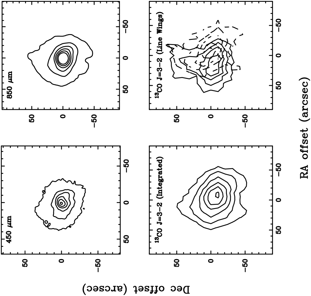
Figure 3: Maps of GL 2591 made at the JCMT, centered at the same position as Figures 1 and 2. The beam size is $7\farcs 5$ FWHM at $450$ $\mu$m and $14\farcs 3$ at $850$ $\mu$m and in ¹³CO, while the peak brightness is $34$ Jy beam^-1 at $450$ $\mu$m, $6.7$ Jy beam^-1 at $850$ $\mu$m and $144$ K km s^-1 in ¹³CO. Top panels: Submillimeter continuum emission, mapped with SCUBA at two wavelengths. Lowest contour and contour interval are $0.4$ and $0.8$ Jy beam^-1 at $850$ $\mu$m and $3.0$ and $6.0$ Jy beam^-1 at $450$ $\mu$m. Bottom panels: Raster map of ¹³CO $J=3\to 2$ emission, obtained with receiver B3i. The left panel shows the total intensity, integrated from -15 to +5 km s^-1, with contours every 20 K km s^-1, starting at 40 K km s^-1. The right panel shows the line wings, integrated from -9 to -15 km s^-1 (solid contours), and from +5 to -3 km s^-1 (dashed contours). Lowest contour and contour interval is 5 K km s^-1 for both velocity ranges.

Figure 3 shows the ¹³CO $J=3\to 2$ map of GL 2591, both in the line wings and integrated over the entire profile. Also shown are $450$ and $850$ $\mu$m continuum observations with the Submillimeter Common User Bolometer Array (SCUBA) at the JCMT, provided by M. van den Ancker and G. Sandell (private communication). The lowest contour drawn for the ¹³CO wing emission, $5$ K km s^-1, is the brightness expected for the molecular cloud surrounding the star-forming region, assuming T${}_{\rm kin}=15$ K, $n=10^{4}$ cm^-3, N(¹³CO)$=1.7\times 10^{16}$ cm^-2 ($N({\rm H}_{2})=10^{22}$ cm^-2) and $\Delta V=2$ km s^-1. The gas and dust tracers agree reasonably well on the extent of the dense molecular cloud core. The diameter at which the intensity has dropped to half its peak value is $\approx 20^{\prime\prime}$ in both continuum maps, measured both N-S and E-W. The ¹³CO diameter is closer to $\approx 30^{\prime\prime}$, but the map of the line wings demonstrates that this elongation is due to the outflow. Data from the KAO scanning photometer at $50$ and $100$ $\mu$m (P. Harvey, private communication) indicate a source diameter of $\approx 20^{\prime\prime}$. Based on these observations, we conclude that the star-forming core is confined to a region of radius $\approx 30^{\prime\prime}$, or $30,000$ AU at 1 kpc. This estimate is accurate to a factor of 2 or so, sufficient to be a useful constraint for the models to be developed in § 4. Although the circumstellar envelope may extend to larger radii, the density and temperature drop to levels that produce little emission in most of the tracers used in this study.

3.4 Infrared Lines and Velocity Structure

Figure 4 presents the calibrated infrared spectra. The apparent emission features in the $2155$ cm^-1 setting are due to the use of the Moon as the reference object (see § 2.3). All absorption features were identified as rovibrational lines of CO and ¹³CO using frequencies calculated from the Dunham coefficients of Farrenq et al. (1991). In the $2155$ cm^-1 setting, which has the highest signal-to-noise ratio, lines of vibrationally excited CO are detected, which are marked with CO* in Figure 4. Table 4 lists the center velocities, FWHM line widths and equivalent widths of all the detected lines, measured by fitting Gaussian profiles to the data. The uncertainty in the line parameters are dominated by errors in continuum placement and by the effects of imperfect cancellation of telluric features.

The ¹²CO fundamental band profiles are very broad and asymmetric, which prohibits the fitting of a Gaussian or Voigt profile. The strongest absorption occurs at v_LSR $=(-21.5\pm 2.6)$ km s^-1, at which position ¹³CO absorption is also detected. From spectra covering many more lines than this work but at a lower velocity resolution, Mitchell et al. (1989) derived a temperature of $200$ K and a CO column density of $6.6\times 10^{18}$ cm^-2 for this gas component, which they called a “$-28$ km s^-1 component”. The line width measured here, $\approx 22$ km s^-1, is larger than the value of $12.5$ km s^-1 by Mitchell et al., so that the column density may also be higher. Our limited line coverage does not allow an accurate measurement of the column density. This component may be related to the outflow seen in the CO rotational lines, for which a temperature of ${{}_{>}\atop{{}^{\sim}}}100$ K was found in § 3.3.

The shape of the broad blueshifted wings of the ¹²CO $v=1\leftarrow 0$ lines suggests an origin in a wind. The position where the continuum is reached is measured to be $(-196\pm 3)$ km s^-1, which gives a terminal velocity of $(173\pm 3)$ km s^-1. This value is much lower than the typical terminal velocity of the winds of early B stars measured from ionic ultraviolet lines, $\sim 1500$ km s^-1 (Lamers, Snow & Lindholme 1995), but much higher than the velocities seen in CO rotational emission in this source (Choi, Evans & Jaffe 1993; § 3.3) or in fact in any source in CO rotational emission (Choi et al. 1993; Shepherd & Churchwell 1995, 1996). A velocity of $\approx 200$ km s^-1 is comparable to the velocity of $500$ km s^-1 seen in the [S II] $\lambda 6731$ line by Poetzel, Mundt & Ray (1992), and to the total width of H I infrared recombination lines in objects similar to GL 2591 (Bunn et al. 1995). The range of velocities seen in ¹²CO absorption suggests an origin in envelope gas entrained by the ionized jet. Figure 5 compares the CO and ¹³CO infrared line profiles with those observed in rotational emission with the JCMT and the CSO.

The ¹³CO absorption lines show a second feature at a less negative v_LSR. This gas was also seen by Mitchell et al. (1989), who attributed it to the quiescent molecular cloud core out of which the star formed. However, Mitchell et al. measured a v_LSR of $-8$ to $-11$ km s^-1 for this component, which does not agree with the velocity of rotational lines. We measure v_LSR=$(-5.7\pm 1.0)$ km s^-1, consistent with the velocity of the millimeter emission lines of CO, CS and other molecules, $(-5.5\pm 0.2)$ km s^-1 (§ 3.3). This value was determined from the R(3), R(10) and R(16) lines, which show no contamination by telluric features. Observations of the $v=2\leftarrow 0$ band of CO with Phoenix give velocities similar to those found here (C. Kulesa, private communication). The line width is measured to be $\approx 10$ km s^-1, similar to that found by Mitchell et al., but a factor of $2-3$ larger than the width of the rotational lines in this source (§ 3.3). Because this linewidth is close to our resolution, it may be an overestimate. Thus, we associate the submillimeter emission and infrared absorption lines with the same gas.

4 Physical Structure of the Envelope

In order to analyze the interferometer line and continuum data, a good physical model of the extended envelope is a prerequisite. The first step will be to constrain the temperature structure of the circumstellar envelope, while the second step is to determine the density structure.

4.1 Dust Temperature Structure

The dust temperature in the envelope as a function of distance from the star was calculated with the computer program by Egan, Leung & Spagna (1988). The number density of dust grains was assumed to follow an $r^{-\alpha}$ power law. Initially, trial values of $0.5-2.0$ were used for $\alpha$, but anticipating the constraints on $\alpha$ provided by the CS line emission (§ 4.3), we only present results for $1.0<\alpha<1.5$. The inner radius was fixed at $200$ AU ($0\farcs 2$ at 1 kpc), much smaller than the OVRO beam and small enough that it does not influence the calculated brightness. Based on the maps presented in § 3.3, we used $30,000$ AU as the outer radius of the models. Larger values for the outer radius give the same conclusions. The observed luminosity of $2\times 10^{4}$ L_⊙ is used, and it is assumed that its source is a zero age main sequence star, in which case the effective temperature is $\approx 30,000$ K (Thompson 1984; Schaerer & de Koter 1997; Hanson, Howarth & Conti 1997). However, varying $T_{\rm eff}$ by a factor 2 at constant $L$ (hence varying the stellar radius) changes the computed submillimeter flux density by less than 1%. The stellar spectral type and any contribution from accretion to the luminosity thus cannot be derived from these models.

The program solves self-consistently for the grain heating and cooling as a function of radius. The model consists of 100 concentric spherical shells, roughly logarithmically spaced. No external radiation field was applied. Comparison to observations proceeds by integrating the radiative transfer equation on a grid of lines of sight followed by convolution to the appropriate beam (Butner et al. 1991). The only free parameter in this process is the number density of dust grains at a given radius, or equivalently the total dust mass. This parameter was constrained by JCMT $450$, $850$, and $1100$ $\mu$m fluxes provided by G. Sandell (private communication), obtained in the same manner as described in Sandell (1994). At these long wavelengths, the dust emission is optically thin and least prone to geometrical effects. In addition, the beams are small enough ($\approx 18^{\prime\prime}$ FWHM) that only the dense core is probed. The model is also compared to $60$, $95$, $110$ and $160$ $\mu$m photometry from Lada et al. (1984), observed with the KAO in a 49^′′ beam, and $2-20$ $\mu$m data from Aitken et al. (1988), obtained at UKIRT in a 4$\farcs$2 beam.

Initially, four sets of optical properties were considered for the dust: the models for diffuse cloud dust by Draine & Lee (1984) and Li & Greenberg (1997), and for dense cloud dust by Mathis, Mezger & Panagia (1983) and Ossenkopf & Henning (1994). We use Ossenkopf & Henning’s model grains with thin ice mantles coagulating at a density of $10^{6}$ cm^-3, called OH5 (column 5 of their Table 1). At visual and ultraviolet wavelengths, the opacities are taken from Model 1 from Pollack et al. (1994), which is similar in spirit. The values of the opacity and the albedo at these short wavelengths do not affect the calculated spectrum since all light is absorbed close to the star. We used a radius of $0.1$ $\mu$m for the grains, and a mass density of $2.3$ g cm^-3, the average of the values for silicate and amorphous carbon. We neglect the effect of a distribution of grain sizes, which would cause a range of dust temperatures at a given radius of $\sim 30$ % or less (Wolfire & Cassinelli 1986). Our temperature profiles therefore represent averages over grain populations, as in Churchwell, Wolfire & Wood (1990).

In Figure 6, the calculated dust temperature profiles are presented, with the curve $T=T_{0}(r/r_{0})^{-0.4}$ expected for optically thin dust superposed. Here, $T_{0}$ is the temperature at the outer radius, $28.7$ K. It is seen that inside a radius of $\approx 2000$ AU, the dust temperature lies above the optically thin curve, and becomes weakly dependent on the grain model and on $\alpha$. The location of the outer edge of the model does not influence the results: for instance, doubling the outer radius changes the calculated temperature at a given radius by less than $0.5$ K, and the emergent flux densities by less than $5$ %. The resulting infrared continuum spectra are shown in the top part of Figure 6. Observed and calculated submillimeter flux densities are summarized in Table 5, along with the implied dust masses inside 30,000 AU and the $20$ $\mu$m flux densities. The masses, or equivalently the values of $n_{0}$, were chosen such that the best fit to the JCMT data is obtained. The same models reproduce the KAO data at 60, 95 and 110 $\mu$m to within a factor of $\sim 2$. In contrast, only the models with Mathis et al. dust match the near-infrared data, and none of the models match the interferometric observations at 3000 $\mu$m. These discrepancies are discussed in §§ 4.5 and 5.1.

Close to the star, the calculated dust temperature is high enough (${{}_{>}\atop{{}^{\sim}}}100$ K) for the ice mantles to evaporate off the grains. In the model with $\alpha=1.5$, half of the material along the central line of sight is at temperatures $>150$ K. Evaporation of icy mantles is consistent with the ISO observations of abundant gaseous H₂O and a ratio of gaseous to solid H₂O of unity (Helmich et al. 1996, van Dishoeck et al. 1996). Therefore we considered a fifth dust model, the Ossenkopf & Henning (1994) opacities for the case of bare grains after coagulation at $10^{6}$ cm^-3 (column 2 of their Table 1), which is denoted by OH2 in Table 5. Models with bare grains close to the star and icy grains at large radii (as in Churchwell et al. 1990) require iteration, because the dust temperature and the optical properties become interdependent. Our computer program is not set up to do this. Instead, we present calculations with either type of grain throughout the cloud, which provide limiting cases. It was found that, while the far-infrared brightness is insensitive to the presence of grain mantles, the calculated mid-infrared flux densities are higher using bare grains than using ice-coated coagulated grains, and closer to the observed values (see Table 5). We interpret this result as strong evidence for grain modification by stellar radiation. This interpretation is supported by the $11.2$ $\mu$m polarization feature, which is due to crystalline olivine grains produced by dust annealing (Aitken et al. 1988; Wright et al. 1999).

Although varying $n_{0}$ can make any of the grain models agree with the observed submillimeter continuum emission for either value of $\alpha$, the implied dust masses vary by factors of $2-100$. This discrepancy reflects differences in the absolute value of the grain opacity at submillimeter wavelengths between the various dust models. In § 4.2, it will be shown that only the models with the Ossenkopf & Henning optical properties are consistent with the masses derived from the C¹⁷O emission.

4.2 Dust and Gas Masses: Measuring the Submillimeter Dust Opacity

Given the temperature structure of the dust, the density distribution in the envelope can be constrained from the molecular line data. The line emission of GL 2591 was modeled with a new computer program using the Monte Carlo approach, developed in Leiden by Hogerheijde & van der Tak (in prep.). The new program was extensively tested against the code by Choi et al. (1995), which was used previously by Carr et al. (1995) to model line emission from GL 2591. The program solves for the local radiation field after each photon propagation and then derives the populations in each molecular energy level. After the level populations have been obtained, line profiles are calculated by line-of-sight integration followed by convolution to the appropriate beam. The model consisted of 20 spherical shells, spaced logarithmically. As in the dust models, the outer radius was taken to be $30,000$ AU. The inner radius was chosen small enough as to not influence the results. In particular, the maximum density must exceed the critical density of all modelled lines.

Radial density profiles of the form $n_{0}(r/r_{0})^{-\alpha}$ were considered, with $\alpha$ between $1.0$ and $2.0$. It is assumed that the gas is heated to the dust temperature by gas-grain collisions throughout the envelope; detailed calculations by Doty & Neufeld (1997; their model with $M_{0.1}=100$ M_⊙, $L/L_{\odot}=10^{4}$) show that this assumption is valid within $20,000$ AU from the star. The maximum difference outside this radius is $20$ %, which we will ignore. The temperature structure calculated for the dust for the same value of $\alpha$ was used. The intrinsic (turbulent) line profile was taken to be a Gaussian with a Doppler parameter ($1/e$ width) of $1.6$ km s^-1, independent of radius.

The following isotopic abundance ratios have been used (Wilson & Rood 1994): ¹²C/¹³C=60, ¹⁶O/¹⁷O=2500, ¹⁶O/¹⁸O=500, ³²S/³⁴S=22, ¹⁴N/¹⁵N=270. For H₂CO, the ortho/para ratio was fixed at 3. The rate coefficients for collisional de-excitation as listed by Jansen et al. (1994) and Jansen (1995) have been used. No rate coefficients are available for $T{{}_{>}\atop{{}^{\sim}}}200$ K, except for HCN and CO, and it is assumed that the collisional de-excitation rate coefficients become temperature-independent at high temperatures.

The values of $n_{0}$ found for a given $\alpha$ from the dust emission using various opacity curves were tested by modelling the C¹⁷O $J=2\to 1$ and $3\to 2$ lines observed with the JCMT, which, like the submillimeter continuum, trace the total column density. We assume a CO/H₂ abundance of $2\times 10^{-4}$, as found for warm, dense clouds by Lacy et al. (1994). Chemical effects are unlikely to change the CO abundance by more than a factor of 2 once most of the gas-phase carbon is locked up in CO. Other carbon-bearing molecules are at least $10^{3}$ times less abundant than CO. No solid CO has been detected towards GL 2591 to a gas/solid CO ratio of $>400$ (Mitchell et al. 1990, van Dishoeck et al. 1996). Estimates of the C⁰ and C⁺ column densities are factors of $50-100$ lower than of that of CO (Choi et al. 1994; C. Wright, private communication).

The C¹⁷O emission observed with the JCMT can be matched using a range of values for $\alpha$, with the implied gas masses within a radius of $30,000$ AU ranging from $33$ M_⊙ for $\alpha=1.5$ to $47$ M_⊙ if $\alpha=1.0$. Comparing these numbers to the dust masses from Table 5, it is seen that only the dust opacities for coagulated grains (OH5 and OH2) yield the standard gas-to-dust mass ratio of $100$. This is strong evidence that grain coagulation occurs in circumstellar envelopes. The corresponding density at $30,000$ AU is $1.5\times 10^{4}$ cm^-3 for $\alpha=1.5$ and $4.5\times 10^{4}$ cm^-3 if $\alpha=1.0$. Although the corresponding total masses are lower limits because the power law may extend further out, the ratio of the dust and gas masses is independent of choice of outer radius. Doubling the radius of the model to $60,000$ AU, for instance, gives the same strength for the C¹⁷O lines within $0.5$ K, or $20$%, while the dust emission is even less affected (§ 4.1). The optical depths of the C¹⁷O lines in the central pencil beam of the model vary from $0.06-0.12$ for $\alpha=1.5$ to $0.09-0.15$ if $\alpha=1.0$.

Calculations were also performed for a source distance of 2 kpc, with the model dimensions doubled, a luminosity of $8\times 10^{4}$ L_⊙, and an effective temperature of 37,500 K. The radius where the dust temperature has a certain value is found to double as well, so that the temperature structure is constant in terms of projected size (in arcseconds), but not in linear size (in AU). To match the observed submillimeter continuum flux densities and C¹⁷O line fluxes, the required dust and H₂ masses are four times those for a distance of 1 kpc.

4.3 Density Distribution

The critical densities of the C¹⁷O lines are such that they are useful to constrain the total column density, but not to discriminate between values of $\alpha$. One of the most suitable molecules to do this is CS, which, because of the small spacing of its energy levels and large dipole moment, samples a large range in critical densities within the observable frequency range. Larger values of $\alpha$ imply that more material is at high gas densities, increasing the ratio of high-$J$ to low-$J$ emission. Further, the $J=5\to 4$ and $J=7\to 6$ lines of CS have been observed in several beams, constraining $\alpha$ even better. The same lines are systematically brighter in smaller beams, which is direct evidence for an inward increase of the density. Indeed, our data and those of Carr et al. (1995) rule out a constant density model. The H₂CO lines all have critical densities of $10^{5}-10^{6}$ cm^-3, and are primarily sensitive to the temperature structure (e.g., Mangum & Wootten 1993, van Dishoeck et al. 1993). Specific H₂CO line ratios can therefore act as a check on the assumption that the kinetic temperature equals the dust temperature. The observed HCO⁺ and HCN lines also have critical densities in the $10^{5}-10^{7}$ cm^-3 range and can be used as checks on the derived density structure. For each combination of $\alpha$ and $n_{0}$, we first calculated the temperature structure using the OH5 dust opacities, and then ran Monte Carlo models for the line emission, tuning the molecular abundances to minimize the difference between observed to synthetic line fluxes. The quality of the fit was measured using the quantity $\chi^{2}$ as defined by Zhou et al. (1991). The uncertainty in the data was taken to be $30$% for all lines except those in the $490$ GHz window, where calibration is difficult, and those obtained in beams $>20^{\prime\prime}$ FWHM with the CSO and NRAO telescopes, which have larger pointing errors and may suffer from beam dilution. These latter lines have an estimated accuracy of $50$%.

It was found that $\chi^{2}$ has a minimum for $\alpha=1.0-1.5$, especially for CS and C³⁴S. With $\alpha<1.0$, very little material is at high densities, giving insufficient excitation of the high-$J$ lines. These are well matched for $\alpha{{}_{>}\atop{{}^{\sim}}}1.5$, but now the low-$J$ lines are a factor of $\sim 2$ weaker than observed. Intermediate values of $\alpha$ provide the observed ratio of low-$J$ to high-$J$ emission and hence the lowest $\chi^{2}$. The best-fitting model has $n=3.5\times 10^{4}(r/30,000{\rm AU})^{-1.25}$ cm^-3, and an H₂ mass of 42 M_⊙. In the case of H₂CO, the minimum of $\chi^{2}$ is not as pronounced, which confirms that the temperature of the molecular gas is close to that of dust, and reflects our finding that the dependence of the dust temperature profile on density structure is small (Figure 6). The $\chi^{2}$ for HCN does not increase for $\alpha>1.5$, suggesting that this molecule is confined to the inner parts of the source, where the density is high. With only 3 observed lines, HCO⁺ is not a sensitive probe of $\alpha$.

The best-fitting abundances are $5\times 10^{-9}$ for CS, $2\times 10^{-9}$ for H₂CO, $2\times 10^{-8}$ for HCN and $1\times 10^{-8}$ for HCO⁺. The calibration of the data would give abundances to $20$% precision, but the major source of error is the CO abundance, leading to an absolute uncertainty of a factor of 2. The abundances are an order of magnitude larger than those derived by Carr et al. (1995), because the H₂ column density of our model is lower. The abundance ratios relative to CO are unchanged, however, so that their discussion and conclusions are not affected. The Carr et al. density structure was not constrained with a column density tracer, leading to a CO abundance of only $2\times 10^{-5}$. Since no significant depletion of CO in ice mantles is observed toward GL 2591, this solution now appears less realistic. In addition, the densities in the models presented here are lower because the temperatures are higher. While Carr et al. used an $r^{-0.4}$ temperature structure, the actual temperature found from our dust modelling is higher in the inner region. We conclude that a calculation of the temperature structure is a prerequisite for a determination of the density structure and chemical composition of high mass cores.

The value of $\alpha$ that fits the CS data best, $\alpha=1.25$, is not predicted by theoretical considerations, but it may result from the averaging out of radial substructure. In very young objects, the central part of the cloud should be undergoing infall (for which $\alpha=1.5$), while further out, the original density profile is maintained. In this interpretation, the data require that the density law of the pre-collapse state is flatter than $r^{-1.5}$, and thus significantly flatter than the $r^{-2}$ law expected for thermally supported clouds. Collapse in an initially logotropic sphere (McLaughlin & Pudritz 1997), with $\alpha\sim 1$ before collapse, might reproduce the data. An average value of $\alpha=1.25$ may also arise in more evolved stages, where even the outer regions are all infalling ($\alpha=1.5$), while at the center, heating and winds from the star push material out, causing an overall flattening of the density structure (i.e., decrease the average $\alpha$).

4.4 Comparison to Infrared Data and Alternative Models

Another test of the power law model is a comparison to infrared absorption line observations, which probe scales down to the point where the observed $4.7$ $\mu$m continuum forms. The high brightness of this continuum is likely due to deviations from a spherical shape as discussed in § 4.5. Lada et al. (1984) fit the emission at $\lambda\leq 13$ $\mu$m with a shell of angular size 0$\farcs$06, and speckle observations at 2.2 $\mu$m give a size $<$0$\farcs$02 (Howell, McCarthy & Low 1981). These numbers are quite uncertain, so we adopt a size of 0$\farcs$1, or 100 AU, for the minimum radius probed by the infrared absorption, which is much smaller than can be probed with the radio data.

Plotted in Figure 7 is the column density implied by our best-fitting spherical power law model in a pencil beam from cloud center to edge in the ¹³CO rotational levels up to $J=25$ and the HCN levels up to $J=11$, divided by their statistical weights. Superposed are infrared observations for the v_LSR$=-5.7$ km s^-1 component of ¹³CO from Mitchell et al. (1989). The higher dispersion data presented in this work are not shown since we have only a few lines and they agree with the equivalent widths of Mitchell et al. (1989). The model points have been scaled to a total ¹³CO column density of $2.1\times 10^{17}$ cm^-2, the value derived by Mitchell et al. from a two-temperature fit to these data. This scaling accounts for the difference in line width of a factor of 5 between the rovibrational and the rotational lines. The observed populations of energy levels $\sim 1000$ K above ground are seen to be reproduced to a factor of $\approx 3$, even though the highest temperature in the model is only $350$ K, which illustrates that temperatures determined from rotation diagrams do not directly reflect the kinetic temperature. The observed column density in high-$J$ levels is even better matched with $\alpha=1.5$, but this model falls short of the low-$J$ population by an order of magnitude. The opposite is true for $\alpha=1.0$; the conclusion is that both millimeter and infrared observations on average support the value $\alpha\approx 1.25$. The factor of 3 discrepancy between data and model is somewhat larger than the scatter in the data, and the two-temperature model by Mitchell et al. (1989) provides a better fit. We interpret this fact as evidence for a nonspherical geometry, which we discuss in more detail in the next section. In the case of CO, unlike HCN, infrared pumping is unlikely to contribute to the excitation, since the radiation field at the lowest-frequency vibrational band of CO at $4.7$ $\mu$m is weak (Fig. 6).

To see if core-halo models can also match the rotational emission line data, models have been run which employ the two-component structure derived by Mitchell et al. (1989, 1990) from the ¹³CO data shown in Figure 7. The halo and the core have temperatures of 40 K and 1000 K and CO column densities of $7.2\times 10^{18}$ cm^-2 and $5.6\times 10^{18}$ cm^-2, respectively. The requirement that the excitation is thermalized leads to typical sizes of the core of $3^{\prime\prime}$ and of the halo of $\leq 60^{\prime\prime}$. Such models are unable to match the observed strengths of the rotational lines, unless the abundances in the core are higher than in the halo. As an example, the CS and C³⁴S line profiles can be fitted for a core with diameter $3^{\prime\prime}$, $n$(H₂)=$2.5\times 10^{6}$ cm^-3 and a CS abundance of $1\times 10^{-8}$, and a halo with diameter $48^{\prime\prime}$ (0.23 pc), $n$(H₂)=$2\times 10^{5}$ cm^-3 and a CS abundance of $3\times 10^{-9}$. These models illustrate the effect of different physical structures on the inferred abundances. Further observational and theoretical research on the physical processes leading to such a core-halo structure is needed. Spectra at positions away from the center should be able to distinguish between power laws and core-halo models, but currently available spectra do not clearly rule out core-halo models.

4.5 Two-dimensional Models

Although the model developed in §§ 4.1- 4.3 matches the molecular line emission and the photometry in the mid-infrared to submillimeter range well, several other observations of GL 2591 remain unexplained. First, all dust models except that of Mathis et al. (1990) fail to reproduce the near-infrared ($2.3-10$ $\mu$m) part of the spectrum. In low-mass objects, bright near-infrared emission is sometimes ascribed to thermal dust emission from a hot circumstellar disk (e.g., Adams, Lada & Shu 1987), and sometimes to scattered light in the case of a disk seen edge-on (e.g., Burns et al. 1989). For less embedded massive stars, it has been attributed to dust inside an ionized region $10-20$ AU from the star, where resonantly scattered Ly$\alpha$ photons heat the dust to $\sim 1000$ K (Wright 1973; Osterbrock 1991). However, all these explanations require a low opacity of the spherical envelope, since otherwise the hot region will be obscured by cold foreground dust (Butner et al. 1991, 1994). For instance, at $3.6$ $\mu$m, the models presented in Figure 6 have optical depths of $1.5-15$ for $\alpha=1.0$ and $3.5-36$ for $\alpha=1.5$. It is more likely that the failure of the other models indicates a deviation from spherical symmetry which provides a low-opacity pathway along our line of sight. The optical depth at $3.6$ $\mu$m of the Mathis et al. model is a factor of 3 lower than that of the OH2 model. Imaging of GL 2591 at $2.2$ $\mu$m (Tamura et al. 1991) shows, in addition to the bright point source, a loop of emission extending $5^{\prime\prime}$ to the West. This feature is interpreted as a limb-brightened cavity cleared by the outflow. The loop, also seen in VLA observations of NH₃ by Torrelles et al. (1989), is indeed coincident with the blue outflow lobe (see Figure 3), i.e., the one directed towards us.

Second, although the $\alpha=1.25$ model reproduces the total fluxes of all our observed rotational lines, the synthetic line profiles of CS, HCN, HCO⁺ and ¹³CO are self-absorbed, contrary to observation. This same problem was encountered by Little et al. (1994) in their study of G34.3, but their solution, artificially lowering the ¹²C/¹³C ratio to $\approx 20$, is not satisfactory. Geometric effects are more likely to play a role, since they affect only the more opaque transitions. The deviation from spherical symmetry can either be global, e.g. in a cavity formed by the stellar wind, or local, as unresolved density variations, so that CS traces high-density “clumps” embedded in a lower-density medium traced by CO. Alternatively, radial variations in the molecular abundances can fix up the line shape. It is not the goal of this paper to distinguish between these effects, which to first order do the same, namely decrease the line opacity. However, large-scale geometry must play some role as demonstrated by the near-infrared emission from the dust, which is insensitive to both chemistry and clumping.

A third, albeit weaker, piece of evidence for a nonspherical geometry is provided by the infrared recombination lines of H I. Tamura & Yamashita (1992) detected Br$\gamma$ emission at the infrared continuum position, with a flux of $8.2\times 10^{-17}$ W m^-2 in a $(2.9\times 4.3)^{\prime\prime}$ beam, a factor of $5-10$ weaker than in similar objects (Bunn et al. 1995). The Br$\gamma$ emission was found to be extended well beyond the radio source: integrated over a $(10\times 16)^{\prime\prime}$ area, the Br$\gamma$ flux is $2.2\times 10^{-16}$ W m^-2. The Br$\alpha$ flux is $<2.3\times 10^{-15}$ W m^-2 in an $11^{\prime\prime}$ beam (Simon et al. 1979), consistent with the Br$\gamma$ to Br$\alpha$ ratio of $0.35$ for standard “case B” recombination, so that scattering is probably unimportant at $2.16$ $\mu$m. Using the fact that the SW continuum source (Figure 1) is an optically thin H II region, Tamura & Yamashita set a lower limit to the extinction towards the SW source of $A_{V}>40$ mag, implying that the SW source is located behind the GL 2591 molecular cloud. The extinction towards the infrared source is not as straightforward to calculate since the nature of the extended emission is not clear (Tamura & Yamashita 1992). In addition, the relation between radio continuum and near-infrared H I line emission is complex when the realistic case of a non-spherical wind with partial ionization is considered (Natta & Giovanardi 1993). The ionized emission from massive young stars with a weak radio continuum such as GL 2591 warrants further study, but is outside the scope of this paper.

The effect of a low-density cone around the central line of sight was approximated by calculating the molecular excitation in the best-fit spherically symmetric model, but with the density set to zero in a cone of opening half-angle $\theta$ around the central line of sight. The outflow axis was assumed to extend all the way from the inner to the outer radius of the model, so that the model cannot be expected to fit the data in detail, because cold gas is seen in absorption towards this source. Synthetic spectra are obtained by performing radiative transfer integrations through this two-dimensional model followed by convolution to the appropriate telescope beam. The results are compared to the spherical case in Figure 8 for a value of $\theta=30^{\circ}$, which gave somewhat better fits to the observations than $\theta=15^{\circ}$, $45^{\circ}$ or $60^{\circ}$. We conclude that there is ample evidence that the circumstellar material is not spherically distributed and that a low-opacity pathway close to our line of sight has important effects on the source’s appearance.

5 Modeling the interferometer data

Using the physical structure of the gas and dust in the extended envelope derived in the previous section, we will now investigate if the best spherical model can also reproduce the interferometer line and continuum data. We do not attempt to calculate the emission from a two-dimensional model since this requires specifying a source function (viz. temperature and density) in addition to an optical depth. This introduces additional free parameters which cannot be independently constrained.

5.1 Continuum emission

Unlike the case for single-dish observations, comparison of models with interferometer data cannot proceed by calculating the total emission within the beam. The measured flux densities in Table 2 are based on a deconvolution with the CLEAN algorithm, which aims to find point sources. In observations of extended sources at high frequencies, a large fraction of the emission is on angular scales larger than that corresponding to the shortest antenna spacing. For resolved objects, the models must be sampled and deconvolved in a manner identical to the interferometer data, but since GL 2591 appears circularly symmetric in our maps (Figures 1 and 2), a simple one-dimensional comparison in the Fourier or $uv$ plane is sufficient.

Figure 9 shows the calculated visibility function of the $\alpha=1.0$ and $\alpha=1.5$ dust models, together with the observations. To obtain the visibility function from the data at $86-115$ GHz, we subtracted the SW source from the $uv$ data, shifted the phase center to the infrared source, and binned the data in annuli about the source. At $226$ GHz, the SW source was not subtracted. The error bars in the plot reflect only the 1$\sigma$ spread in the data points. The bins at the shortest and longest baselines have considerably more uncertainty because these regions of the $uv$ plane are the most sparsely sampled by the interferometer. Note that the high flux observed on the shortest baselines does not show up in the images in Figure 1, illustrating the limitations of the deconvolution algorithm.

From Figure 9, the model is seen to reproduce the visibility data only on the shortest spacings. On baselines ${{}_{>}\atop{{}^{\sim}}}15$ k$\lambda$, the observed $86-115$ GHz flux lies a factor of $3-4$ above the model value. If the emission is resolved at the largest spacing, the radius of the compact source is $\approx 1000$ AU, in which case the temperature of an opaque source equals the brightness temperature of $\approx 1$ K. However, such a low temperature at this radius is physically untenable because the warmer envelope fills most of the sky as seen from the source and acts as an oven. Hence emission on this scale must be optically thin, and the compact source must be at least as warm as the ambient envelope. The 86 and 106 GHz data are actually consistent with an unresolved source. In this case, we derive a lower limit to the source radius by following the curve $T_{B}(r/1000\ {\rm AU})^{-2}$ to where it intersects the temperature curve calculated for the envelope. This leads to an estimated radius of ${{}_{<}\atop{{}^{\sim}}}30$ AU and a temperature of ${{}_{>}\atop{{}^{\sim}}}1000$ K for an opaque source. Alternatively, the compact emission may be due to a steepening of the density gradient for radii $<1000$ AU. The $226$ GHz data are uncertain, but appear well matched by the model power law envelope, which “outshines” any possible compact source. Higher-resolution interferometry in the $100$ GHz band is needed to put additional constraints on the size and orientation of this compact component.

5.2 HCN line emission

Infrared observations of GL 2591 by Carr et al. (1995) and by Lahuis & van Dishoeck (1997) imply a ${{}_{>}\atop{{}^{\sim}}}100\times$ higher abundance of HCN than found in § 4.3. The HCN column density of $1.5\times 10^{17}$ cm^-2 and excitation temperature $T_{\rm rot}\approx 1000$ K by Lahuis & van Dishoeck should give rise to strong rotational emission. Do we see any emission from the inner region reflected in the interferometer data?

The line emission from the envelope seen by OVRO was modelled using the same approach as for the continuum, motivated by the structureless appearance of the maps in Figure 2. After solving for the molecular excitation, maps of the sky brightness are constructed at several velocities. These are Fourier transformed, and the result is binned in annuli around the center. The results are presented in Figure 10, which compares the observed and modelled $J=1\to 0$ emission of all three HCN isotopes and of C¹⁷O. To avoid confusion with the broad, blueshifted velocity component, as well as with the hyperfine components, the observed emission has been integrated over just $1$ km s^-1, centered on v_LSR$=-5.7$ km s^-1. For HCN and H¹³CN, the model results have been divided by 2 to account for the hyperfine components. The poor match on short spacings is probably due to inadequate sampling, so that the error bar was underestimated.

The OVRO observations of HCN and isotopes show no excess at large spacings over the predictions of the power law model, indicating that the HCN abundance does not increase appreciably on radii down to $1500$ AU, corresponding to the last data point at $80$ k$\lambda$. To avoid the interferometer seeing the extra rotational emission from the hot optically thick HCN observed with ISO, this region must be beam diluted by at least a factor of 100 in the OVRO beam of 3$\farcs$5. Hence, the source radius must be smaller than $175$ AU.

The temperature at $r=1500$ AU exceeds $120$ K (Fig. 6). Therefore, the source of HCN seen on smaller scales by ISO cannot simply be the evaporation of icy grain mantles, since the most refractory (and most abundant) interstellar ice, solid H₂O, evaporates in $\sim 10$ yr when $T{{}_{>}\atop{{}^{\sim}}}100$ K (Sandford & Allamandola 1993). This is consistent with the fact that solid HCN has not been detected down to levels of 3% relative to water ice, or $3\times 10^{-6}$ relative to H₂ (W. Schutte, private communication). The temperature at $175$ AU from the star exceeds 300 K, strongly suggesting that high-temperature chemistry is producing the observed HCN enhancement. One possibility is that most of the oxygen is driven into H₂O at temperatures $>200$ K (Charnley 1997), leaving little atomic O to destroy HCN. The hot HCN seen with ISO is not the inner peak of the power-law envelope because its rotation diagram is nearly flat (indicating $T\sim 1000$ K), whereas the synthetic rotation diagram from the power law model declines substantially over the observed range of lower state energy (Fig. 7, bottom panel), indicating a column-integrated excitation temperature of only $\sim 100$ K. Thus, the hot HCN must arise in a separate, HCN-enriched component, which is probably very hot and dense. The models presented in Figure 7 do not include infrared pumping, however, while our detection of rotational lines of vibrationally excited HCN suggests that this effect may contribute to the excitation. Observations at sub-arcsecond resolution of high-excitation lines are needed to image this chemically active region.

6 Conclusions

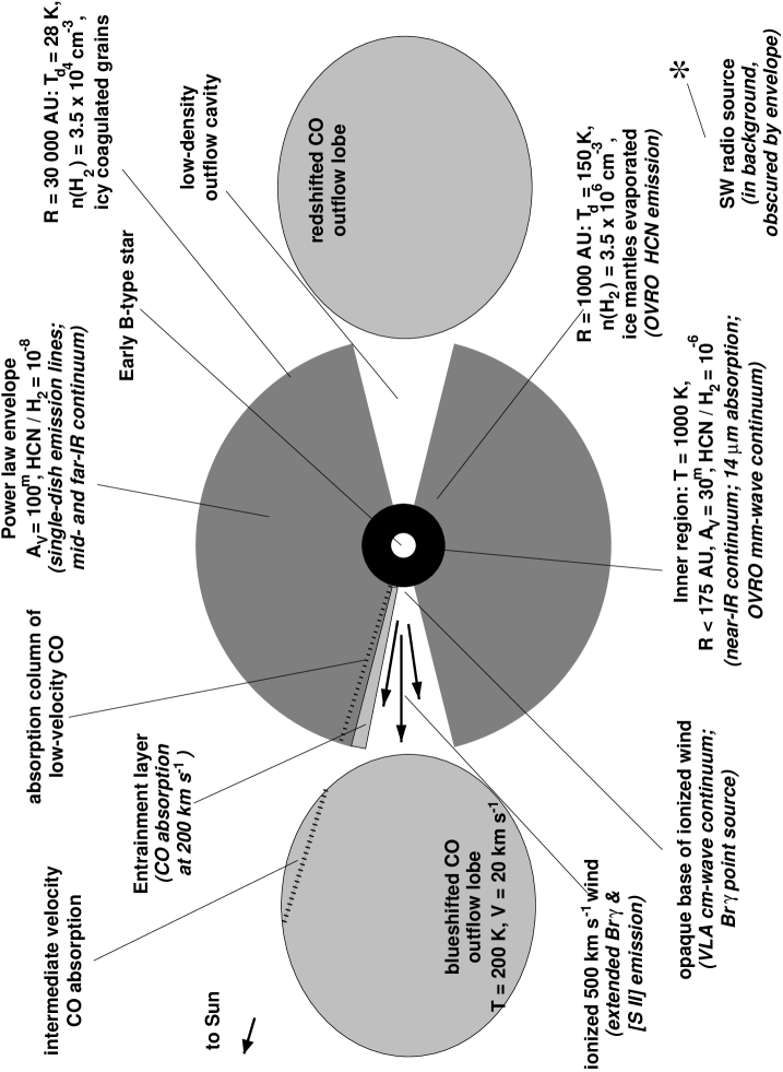
Figure 11: Schematic drawing of GL 2591, not to scale, with the observational characteristics of the various physical components indicated. Velocities are in the rest frame of the source; subtract $5.7$ km s^-1 to convert to the LSR scale.

In this paper, the circumstellar environment of the massive young star GL 2591 ($L=2\times 10^{4}$ L_⊙, $D=1$ kpc) has been studied through a variety of infrared, single-dish submillimeter, and interferometric observations. The data are modelled using a two-step method. The temperature structure is first calculated with a dust radiative transfer code solving for the heating and cooling balance of the grains as a function of distance to the star. The density structure is then obtained with a Monte Carlo calculation of the excitation of molecular emission lines, using the temperature distribution calculated by the dust code. Subsequently, this model for the envelope on 30,000 AU scales is compared with the interferometric and infrared spectroscopic data, which trace scales from 100 to 30,000 AU. Our main conclusions are written down below, and sketched in Figure 11.

1. The C¹⁷O $J=2\to 1$ and $J=3\to 2$ lines observed with the JCMT indicate $A_{V}\approx 100$ mag, or a circumstellar mass of $\approx 42$ M_⊙ contained within a volume of radius $30,000$ AU around the star.

2. The radiative transfer calculations for the dust indicate that the temperature is enhanced over the $T\propto r^{-0.4}$ relation valid for optically thin dust inside a radius of $2000$ AU. The dust mass, obtained by fitting the far-infrared and submillimeter data, depends strongly on choice of submillimeter dust opacity. Consistency with the gas mass derived from C¹⁷O requires a high value for the opacity; agreement to better than $50$% is found adopting the opacities by Ossenkopf & Henning (1994) for dust grains which have coagulated and acquired ice mantles in the dense, cold outer parts of the circumstellar envelope.

3. Single-dish observations of the CS and C³⁴S $J=2\to 1$ through $10\to 9$ lines can be modelled successfully with a power-law density structure $n=n_{0}r^{-\alpha}$. The best match to the v_LSR$=-5.7$ km s^-1 lines is found for $\alpha=1.25\pm 0.25$ and $n_{0}=(3.5\pm 1)\times 10^{4}$ cm^-3 at a radius of $30,000$ AU. The gas temperature as traced by emission lines of H₂CO is found to follow the dust temperature closely. The derived value of $\alpha$ is between the values expected for free-fall collapse and nonthermal support, suggesting a combination of these dynamical states within the single-dish beams.

4. At $\sim 1500$ AU from the star, the calculated dust temperature exceeds $120$ K, so that the ice mantles are expected to have evaporated. Models with the ice removed from the grains indeed give much better fits to the strong mid-infrared emission observed than do models with ice-coated grains. Evaporation of the ice is also required by the gas/solid ratios of H₂O and CO observed in the infrared.

5. The spherical power law model does not give a good match to the strong near-infrared emission, to the line profiles of ¹³CO, CS, HCN and HCO⁺, and to the infrared recombination lines of H I. This suggests a deviation from spherical symmetry leading to a decrease in opacity along the central pencil beam by a factor of $\approx 3$, such as a low-density cone evacuated by the molecular outflow, which is directed almost towards us. Models with an opening angle of the cone of $\approx 30^{\circ}$ reproduce the CS, HCN and HCO⁺ line profiles. It appears that the star is actively shaping its local environment.

6. We confirm the triple velocity structure in the $4.7$ $\mu$m lines of CO reported by Mitchell et al. (1989), but measure velocities of $(-23\pm 3.2)$ and $(-5.6\pm 1.0)$ for the discrete ¹³CO components, and a terminal velocity of $(173\pm 3)$ km s^-1 for the high-velocity wind. This velocity suggests an origin in envelope gas entrained by the ionized jet seen in Br$\gamma$ and [S II]. Due to the finite size of the background continuum, both the quiescent envelope gas (at $-5.6$ km s^-1) and the entrainment layer (seen as the wind feature) are visible in absorption. The ¹³CO absorption at $-21.5$ km s^-1 arises in the foreground outflow lobe, which gas also produces the wings on the rotational emission lines of CO, CS, H₂CO, HCN and HCO⁺. The ¹³CO excitation seen in infrared absorption as well as the strong CO $J=6\to 5$ emission indicates a temperature of the outflow lobe of $\sim 200$ K.

7. The OVRO continuum data, when compared to the envelope model derived from the single-dish data, reveal a compact source of radius $<1000$ AU, brightness temperature of $\approx 1$ K and spectral index $\approx 1.7\pm 0.3$. No constraints on the geometry of this component are available. One possibility is optically thick, thermal emission from a $\sim 1000$ K, $30$ AU radius region of hot dust. Alternatively, the compact emission may reflect a steepening of the density gradient on radii $<2000$ AU.

8. ISO observations by Lahuis & van Dishoeck (1997) indicate an HCN abundance of $\sim 10^{-6}$ and an excitation temperature of $\approx 1000$ K. The OVRO HCN data are consistent with the power law envelope model, implying that the HCN abundance remains at the $10^{-8}$ level down to radii of $\sim 1500$ AU. Therefore, the enhancement of HCN does not start until well after temperatures of $120$ K are reached, considerably above the evaporation temperature of any interstellar ice. The enhancement seems to occur within $175$ AU from the star where $T>300$ K, suggesting that high-temperature gas-phase chemistry is important. This region is further evidence for the effect of the star on its environment.

Table 1: Parameters of OVRO observations.

	Setting 1	Setting 2	Setting 3
Frequency (GHz)	86	106	115/226
Observation date	27sep95/16dec95	29sep95/02jan96/03jan96	01feb97/24mar97/01jun97
Configuration	LR/EQ	LR/EQ/EQ	LR/HR/LR
Time on-source (min.)	380/460	420/180/235	260/140/280
Wide mode:
Resolution (km s-1)	0.87	0.71	0.65
Coverage (km s-1)	112	90.5	83.4
Lines	HCN $J=1\to 0$,	CH3OH $3_{1}-4_{0}$ A+,	CO, C17O
	SO $J=2_{2}-1_{1}$	SO2 $10_{1,9}-10_{0,10}$	$J=1\to 0$
Narrow mode:
Resolution (km s-1)	0.44	0.35	0.33
Coverage (km s-1)	27.9	22.6	20.9
Lines	H13CN, HC15N	CH3OH $11_{-1}-10_{-2}$ E,	CO, C17O
	$J=1\to 0$	H2CS $3_{12}-2_{11}$	$J=1\to 0$
Continuum bandwidth	0.5 GHz	0.5 GHz	1.0 GHz
Longest baseline (k$\lambda$)	70	84	95/90
Synthesized beam FWHM:
Continuum	$(2.4\times 1.8)^{\prime\prime}$, $-88^{\circ}$	$(2.0\times 1.5)^{\prime\prime}$, $-88^{\circ}$	$(2.3\times 1.5)^{\prime\prime}$, $-69^{\circ}$ /
			$(1.9\times 1.4)^{\prime\prime}$, $-43^{\circ}$
Lines	$(3.7\times 3.0)^{\prime\prime}$, $-73^{\circ}$	$\cdots$	$(3.4\times 2.7)^{\prime\prime}$, $-54^{\circ}$
Map rms (mJy beam-1)	60 (CO, HCN)	80-100 (H13CN, HC15N)	1.7 (continuum)
(all settings)

Table 2: Positions and Flux Densities of Radio Sources in GL 2591.

	RA (1950)	Dec (1950)	Flux Density	Reference
	20h27m	+40∘01′	(mJy)
SW source
VLA 5 GHz	35s.613 (0.007)	10′′.4 (0.1)	79 (2.0)	Campbell (1984)
VLA 8.4 GHz	35s.659 (0.007)	10′′.4 (0.1)	82 (8.0)	Tofani et al. (1995)
OVRO 87 GHz	35s.63 (0.004)	10′′.4 (0.1)	87 (1.4)	This work
OVRO 106 GHz	35s.62 (0.004)	10′′.4 (0.1)	71 (1.2)	This work
OVRO 115 GHz	35s.63 (0.01)	10′′.4 (0.1)	93 (2.5)	This work
NE source
VLA 5 GHz	35s.963 (0.007)	14′′.8 (0.1)	0.4 (0.1)	Campbell (1984)
VLA 8.4 GHz	35s.975 (0.007)	14′′.7 (0.1)	0.5 (0.1)	Tofani et al. (1995)
OVRO 87 GHz	35s.95 (0.004)	14′′.9 (0.1)	29.5 (0.8)	This work
OVRO 106 GHz	35s.93 (0.003)	14′′.9 (0.1)	38.7 (0.7)	This work
OVRO 115 GHz	35s.97 (0.009)	14′′.8 (0.1)	52.9 (1.5)	This work
OVRO 226 GHz	35s.88 (0.013)	14′′.7 (0.2)	151 (4.5)	This work
2.2 $\mu$m	36s.00 (0.09)	15′′ (1)		Tamura et al. (1991)

Table 3: Gaussian fits to observed submillimeter emission lines

Molecule	Transition	Frequency	$\int T_{\rm MB}dV$	$\Delta V$	$T_{\rm mb}$	Telescope / Date
		(MHz)	(K km s-1)	(km s-1)	(K)
CI	${}^{3}P_{1}-^{3}P_{0}$	492160.7	85.8	8.64	9.34	JCMT Oct ’95
	${}^{3}P_{1}-^{3}P_{0}$	-5.4	23.2	3.08	7.09
		-8.3	68.9	11.56	5.60
13CO	3-2	330588.1	224.1	5.15	40.86	JCMT May ’95
	3-2	-5.5	136.7	3.33	31.38
		-7.0	111.0	8.77	14.64
	6-5	661067.4	236.0	5.51	40.3	CSO May ’95
	6-5	-5.5	113.5	3.75	28.5
		-6.5	140.3	8.81	15.0
C17O	2-1	224714.4	9.6	4.14	2.17	JCMT May ’95
	2-1	-5.7	4.4	2.75	1.50
		-7.2	5.6	5.36	0.98
	3-2	337060.9	14.7	3.28	4.19	JCMT May ’95
	3-2	-5.7	6.03	2.14	2.66
		-6.6	9.10	4.90	1.74
CS	5-4	244935.6	25.2	3.62	6.55	JCMT Oct ’95
	5-4	-5.6	11.7	2.45	4.46
		-6.5	14.6	5.13	2.70
	7-6	342883.0	22.8	3.32	6.47	JCMT May ’96
	7-6	-5.3	10.1	2.25	4.22
		-6.1	13.9	4.70	2.77
C34S	5-4	241016.2	3.41	3.16	1.01	JCMT May ’96
	7-6	337396.7	1.86	2.73	0.64	JCMT May ’95
CS (v=1)	7-6	340398.1	-	-	$<$ 0.20	JCMT May ’95
H2CO	$3_{03}-2_{02}$	218222.2	9.84	3.65	2.54	JCMT Oct ’95
	$3_{03}-2_{02}$	-5.8	4.51	2.17	1.96
		-6.5	6.29	6.20	0.95
	$3_{22}-2_{21}$	218475.6	2.57	3.83	0.63	JCMT Oct ’95
	$3_{12}-2_{11}$	225697.8	14.44	3.81	3.56	JCMT May ’95
	$3_{12}-2_{11}$	-5.6	8.57	2.77	2.90
		-6.6	7.11	6.80	0.98
	$5_{15}-4_{14}$	351768.7	12.86	3.58	3.38	JCMT May ’95
	$5_{05}-4_{04}$	362735.9	5.71	3.21	1.67	JCMT May ’95
	$5_{24}-4_{23}$	363945.9	3.55	3.57	0.93	JCMT May ’95
	$5_{42/41}-4_{41/40}$	364102.8	1.00	4.96	0.19	JCMT May ’95
	$5_{33}-4_{32}$	364275.2	4.24	4.41	0.90	JCMT May ’95
	$5_{32}-4_{31}$	364289.0	4.34	4.86	0.84	JCMT May ’95
	$7_{17}-6_{16}$	491968.9	9.98	4.76	1.96	JCMT Oct ’95
H${}_{2}^{13}$CO	$5_{05}-4_{04}$	353811.8	-	-	$<$ 0.20	JCMT May ’96
HCN	4-3	354505.5	45.7	4.60	9.33	JCMT May ’95
	4-3	-5.1	24.7	3.47	6.67
		-6.4	23.1	6.52	3.33
HCN ($\nu_{2}=1$)	$4_{1}-3_{1}$	354460.4	2.47	5.38	0.43	JCMT May ’95
H13CN	1-0	86340.2	1.78	3.63	0.26	KP12m Nov ’95
	3-2	259011.8	5.51	4.19	1.23	JCMT Oct ’95
	4-3	345339.8	8.64	4.94	1.64	JCMT May ’95
HC15N	1-0	86055.0	0.31	3.76	0.08	KP12m Nov ’95
	3-2	258157.3	2.39	4.38	0.51	JCMT Oct ’95
	4-3	344200.3	3.10	4.50	0.65	JCMT May ’95
HCO+	4-3	356734.3	91.8	4.56	19.0	JCMT May ’96
	4-3	-5.4	55.8	3.45	15.2
		-6.7	44.2	8.22	5.03
H13CO+	3-2	260255.5	6.18	3.17	1.83	JCMT Oct ’95
	3-2	-5.5	5.45	2.66	1.93
		-8.1	0.88	2.04	0.40
	4-3	346998.5	5.45	2.45	2.08	JCMT May ’96
	4-3	-5.4	4.37	2.11	1.95
		-7.1	1.43	3.62	0.37
HC18O+	4-3	340633.0	-	-	$<$ 0.15	JCMT May ’96

Note. — Uncertainties of the line flux and brightness are $30$% for JCMT observations, due to calibration; the less stable pointing of the CSO and NRAO leads to an error estimate of $50$%. Peak velocities and line widths are accurate to $\approx 0.1$ km s^-1.

Table 4: Measured Properties of the Infrared Lines.

Line	Rest frequency	Observed frequency	LSR Velocity	Line FWHM	Equivalent Width
	cm-1	cm-1	km s-1	km s-1	$10^{-3}$ cm-1
12CO $v=1\leftarrow 0$ R(1)	2150.856	2151.199	-19.1	$\cdots$	1.732
		2152.978	-267	$\cdots$	-0-
R(2)	2154.596	2154.938	-18.9	$\cdots$	1.470
		2156.213	-196	$\cdots$	-0-
R(3)	2158.300	2158.645	-19.2	$\cdots$	1.214
		2159.931	-198	$\cdots$	-0-
P(2)	2135.546	2135.710	-20.8	$\cdots$	2.70
P(3)	2131.632	2131.818	-23.9	$\cdots$	2.81
		2133.024	-194	$\cdots$	-0-
P(7)	2115.629	2115.817	-24.4	$\cdots$	2.408
		2116.605	-136	$\cdots$	-0-
P(8)	2111.543	2111.731	-24.5	$\cdots$	2.120
		2112.933	-195.1	$\cdots$	-0-
12CO $v=2\leftarrow 1$ R(8)	2149.489	2149.688	+1.0	10.2	5.25
R(9)	2152.942	2153.344	-9.3	19.9	16.25
		2153.215	-27.2	19.1	4.60
R(10)	2156.358	2156.566	-1.8	19.2	28.59
R(11)	2159.739	2160.036	-12.5	9.7	4.25
13CO $v=1\leftarrow 0$ R(3)	2110.442	2110.507	-7.0	9.5	33.39
		2110.628	-24.2	22.7	68.90
R(4)	2113.953	2114.043	-10.5	6.7	21.98
		2114.162	-27.4	22.0	57.66
R(5)	2117.431	2117.518	-10.1	18.8	68.86
		2117.628	-25.7	8.1	21.00
R(9)	2131.004	2131.084	-9.0	52.5	50.91
R(10)	2134.313	2134.354	-3.5	23.2	14.99
		2134.535	-28.9	34.8	59.17
R(11)	2137.588	2137.668	-9.0	6.0	3.53
		2137.809	-28.8	20.6	35.57
R(15)	2150.341	2150.612	-9.0	10.7	2.89
R(16)	2153.443	2153.696	-6.5	20.1	8.05
		2153.822	-24.0	24.5	11.69
R(17)	2156.509	2156.805	-12.4	30.0	23.70
R(18)	2159.540	2159.799	-7.2	40.7	25.65

Note. — When measured through profile fitting, velocities and line widths are accurate to $\approx 1$ km s^-1; terminal velocities were estimated by eye and have an uncertainty of 3 km s^-1. Equivalent widths are accurate to $\approx 30$% for clean lines and to $50$% for contaminated lines.

Table 5: Observed and modelled submillimeter flux densities of GL 2591.

Dust model	$\alpha$	Dust Mass	$F_{20}$	$F_{450}$	$F_{800}$	$F_{1100}$
		(M⊙)	(Jy)	(Jy)	(Jy)	(Jy)
LG	$1.5$	$3.22$	$0.22$	$77.9$	$6.75$	$2.62$
LG	$1.0$	$4.46$	$0.22$	$71.3$	$6.20$	$2.47$
DL	$1.5$	$13.34$	$20.8$	$75.3$	$7.30$	$2.70$
DL	$1.0$	$18.47$	$39.8$	$69.6$	$6.77$	$2.56$
MMP	$1.5$	$1.18$	$288.$	$77.8$	$5.30$	$1.89$
MMP	$1.0$	$1.68$	$345.$	$73.2$	$5.01$	$1.83$
OH5	$1.5$	$0.34$	$139.$	$66.9$	$6.12$	$2.62$
OH5	$1.0$	$0.48$	$265.$	$65.3$	$5.97$	$2.62$
OH2	$1.5$	$0.21$	$731.$	$61.6$	$7.71$	$3.57$
OH2	$1.0$	$0.33$	$912.$	$67.8$	$8.47$	$4.00$
Observed:			$733.\pm 147.$	$66.3\pm 3.1$	$8.2\pm 0.24$	$2.93\pm 0.12$

Note. — The $450-1100$ $\mu$m data are JCMT observations by G. Sandell (private communication). Beam FWHM is $18^{\prime\prime}.5$ at $450$ $\mu$m, $17^{\prime\prime}.5$ at $850$ $\mu$m and $18^{\prime\prime}.5$ at $1100$ $\mu$m. The $20$ $\mu$m flux is from Aitken et al. (1988), obtained in a $4^{\prime\prime}.2$ FWHM beam with UKIRT. The grain models are labelled as follows: DL = Draine & Lee (1984), LG = Li & Greenberg (1997), MMP = Mathis, Mezger & Panagia (1983), OH = Ossenkopf & Henning (1994). The masses refer to a volume of radius 30,000 AU.

Figure 1: OVRO continuum maps of GL 2591. The beam FWHM is indicated in the top left corner. Contour levels are 6 to 42 by 12 mJy beam^-1 at 86 GHz, 5 to 35 by 10 mJy beam^-1 at 106 GHz, 10 to 50 by 20 mJy beam^-1 at 115 GHz and 20 to 140 by 40 mJy beam^-1 at 226 GHz. The map center is at R.A. 20^h 27^m 35^s.8, Dec +40^∘ 01^′ 14^′′ (B1950).

Figure 2: Integrated intensity maps (left panels) and spectra (middle panels) of molecular lines observed with OVRO in a $3^{\prime\prime}.5$ beam. The map center is the same as in Figure 1. Lowest contour and contour interval is $130$ mJy beam^-1 (HCN), $110$ mJy beam^-1 (H¹³CN), $80$ mJy beam^-1 (HC¹⁵N), $200$ mJy beam^-1 (CO). The right panels show spectra observed with the NRAO 12m telescope (thin lines) and with OVRO (thick lines), both in a $63^{\prime\prime}$ beam.

Figure 4: Spectra in three wavelength regions near $4.7$ $\mu$m, observed with the Phoenix spectrometer. To eliminate telluric features, the source data are divided by the standard star data (Moon/Vega), scaled to the appropriate air mass. Lines of CO and ¹³CO in the $v=1\leftarrow 0$ band are indicated above and below the spectrum, respectively. Lines in the ¹²CO $v=2\leftarrow 1$ band are denoted with an asterisk.

Figure 5: Submillimeter emission lines (in K) and infrared absorption lines (in relative units) of CO and ¹³CO, observed with the indicated telescopes.

Figure 6: Observed continuum emission from GL 2591 (large open circles) with model fits superposed. In the left panels, the density drops as $r^{-1.0}$ with distance from the star $r$, while in the right panels, it drops as $r^{-1.5}$. Bottom: Calculated dust temperature versus distance from star. The dust models are labeled as follows: OH5 = Ossenkopf & Henning (1994), LG = Li & Greenberg (1997), DL = Draine & Lee (1984) and MMP = Mathis et al. (1983).

Figure 7: Column density per rotational sublevel versus level energy for the best fit spherical power law model, denoted by filled circles. Top: ¹³CO $v=1\leftarrow 0$ band, compared with observations by Mitchell et al. (1989), scaled to their total column density of $2.1\times 10^{17}$ cm^-2. The observational error, $2\times 10^{14}/(2J+1)$ cm^-2, is smaller than the plotting symbol. Bottom: HCN $\nu_{2}$ band, compared with the populations in the case of constant excitation temperatures along the line of sight of 100 and 1000 K. The value of 1000 K was derived from ISO observations by Lahuis & van Dishoeck (1997). All curves have been scaled to N(HCN)$=7.2\times 10^{16}$ cm^-2. The model does not include infrared pumping.

Figure 8: Line profiles of CS and C³⁴S, observed with the JCMT unless otherwise indicated. Dotted line: best fit spherical power law model with $n($H${}_{2})=3.5\times 10^{4}$ (r/30,000 AU)^-1.25 cm^-3, CS/H₂ $=1\times 10^{-8}$. Dashed line: Two-dimensional model with an outflow opening angle of $\theta=30^{\circ}$.

Figure 9: Continuum visibilities observed at 86, 106, 115 and 226 GHz with OVRO, binned in azimuth about the phase center. The dashed line indicates the amplitude bias. The solid line is the visibility function calculated for the power law model fitted to the JCMT continuum data.

Figure 10: As Figure 9, but for the $J=1\to 0$ lines of HCN, H¹³CN, HC¹⁵N and C¹⁷O. The observed emission is integrated over 1 km s^-1.

References

- (1)
- (2) Adams, F.C., Lada, C.J. & Shu, F.H. 1987, ApJ, 312, 788
- (3) Aitken, D.K., Smith, C.H., James, S.D., Roche, P.F. & Hough, J.H. 1988, MNRAS, 230, 629
- (4) Blake, G.A. 1997, in: IAU Symposium 178: Molecules in Astrophysics, ed. E.F. van Dishoeck (Kluwer Academic Publishers), p. 31.
- (5) Blake, G.A., Mundy, L.G., Carlstrom, J.E., Padin, S., Scott, S.L., Scoville, N.Z., & Woody, D.P. 1996, ApJ, 472, L49
- (6)
- (7) Boss, A.P. 1996, ApJ, 469, 906
- (8)
- (9) Bunn, J.C., Hoare, M.G. & Drew, J.E. 1995, MNRAS, 272, 346
- (10)
- (11) Burns, M.S., Hayward, T.L., Thronson, H.A., Jr. & Johnson, P.E. 1989, AJ, 98, 659
- (12)
- (13) Butner, H. M., Evans, N. J., II, Lester, D. F., Levreault, R. M., & Strom, S. E. 1991, ApJ, 376, 636
- (14)
- (15) Butner, H.M., Natta, A. & Evans, N.J., II 1994, ApJ, 420, 326
- (16)
- (17) Cabrit, S., Raga, A., & Gueth, F. 1997, in: Herbig-Haro Flows and the Birth of Low Mass Stars, eds. B. Reipurth & C. Bertout (Kluwer Academic Publishers), p. 163
- (18)
- (19) Campbell, B. 1984, ApJ, 287, 334
- (20)
- (21) Carr, J.S., Evans, N.J., II, Lacy, J.H. & Zhou, S. 1995, ApJ, 450, 667
- (22)
- (23) Charnley, S. B. 1997, MNRAS, 291, 455
- (24)
- (25) Choi, M., Evans, N.J. II, Gregersen, E.M. & Wang, Y. 1995, ApJ, 448, 742
- (26)
- (27) Choi, M., Evans, N.J. II & Jaffe, D.T. 1993, ApJ, 417, 624
- (28)
- (29) Churchwell, E.B. 1993, in: Massive Stars, Their Lives in the Interstellar Medium, eds. J.P. Cassinelli & E.B. Churchwell (ASP Conference Series, Vol. 35), p. 35.
- (30)
- (31) Churchwell, E.B. 1999, in: The Physics of Star Formation and Early Stellar Evolution II, eds. C.J. Lada & N.D. Kylafis (Kluwer Academic Publishers, in press).
- (32)
- (33) Churchwell, E., Wolfire, M.G. & Wood, D.O.S. 1990, ApJ, 354, 247
- (34)
- (35) Dickel, H.R., Wendker, H. & Bieritz, J.H. 1969, A&A, 1, 270
- (36) Doty, S.D. & Neufeld, D.A. 1997, ApJ, 489, 122
- (37) Draine, B.T. & Lee, H.M. 1984, ApJ, 285, 89
- (38) Egan, M. P., Leung, C. M., & Spagna, G. R., Jr. 1988, Comput. Physics Comm., 48, 271
- (39)
- (40) Farrenq, R. Guelachvili, G., Sauval, A. J., Grevesse, N. & Farmer, C. B. 1991, J. Mol. Sp. 149, 375
- (41)
- (42) Genzel, R. & Stutzki, J. 1989, ARA&A, 27, 41
- (43) Hanson, M.M., Howarth, I.D. & Conti, P.S. 1997, ApJ, 489, 698
- (44)
- (45) Hasegawa, T.I. & Mitchell, G.F. 1995, ApJ, 451, 225
- (46) Helmich, F.P., van Dishoeck, E.F., Black, J.H. et al. 1996, A&A, 315, L173
- (47) Hollenbach, D., Johnstone, D., Lizano, S. & Shu, F. 1994, ApJ, 428, 654
- (48)
- (49) Howell, R. R., McCarthy, D. W. & Low, F. J. 1981, ApJ, 251, LL21
- (50) Hunter, T.R., Phillips, T.G. & Menten, K.M. 1997, ApJ, 478, 283
- (51)
- (52) Jansen, D.J. 1995, Ph.D. thesis, University of Leiden.
- (53) Jansen, D.J., van Dishoeck, E.F. & Black, J.H. 1994, A&A, 282, 605
- (54)
- (55) Lacy, J.H., Knacke, R., Geballe, T.R. & Tokunaga, A.T. 1994, ApJ, 428, L69
- (56)
- (57) Lada, C.J., Thronson, H.A., Jr., Smith, H.A., Schwarz, P.R. & Glaccum, W. 1984, ApJ, 286, 302
- (58)
- (59) Lahuis, F. & van Dishoeck, E.F. 1997, in: First ISO Workshop on Analytical Spectroscopy, eds. A.M. Heras, K. Leech, N.R. Trams & M. Perry (Noordwijk: ESA), p. 275.
- (60) Lamers, H.J.G.L.M., Snow, T.P. & Lindholm, D.M. 1995, ApJ, 455, 269
- (61) Li, A. & Greenberg, J.M. 1997, A&A, 323, 566
- (62) Little, L.T., Gibb, A.B., Heaton, B.D., Ellison, B.N. & Claude, S.M.X. 1994, MNRAS, 271, 649
- (63) Lizano, S., & Shu, F. H., 1989, ApJ, 342, 834
- (64) Mangum, J.G. & Wootten, A. 1993, ApJS, 89, 123
- (65) Mathis, J.S., Mezger, P.G. & Panagia, N. 1983, A&A, 128, 212
- (66)
- (67) Matthews, H.E. 1995, in: The James Clerk Maxwell Telescope: a Guide to the Prospective User
- (68)
- (69) McLaughlin, D. E., & Pudritz, R. E. 1997, ApJ, 476, 750
- (70) Mitchell, G.F., Curry, C., Maillard, J.-P. & Allen, M. 1989, ApJ, 341, 1020
- (71) Mitchell, G.F., Hasegawa, T.I. & Schella, J. 1992, ApJ, 386, 604
- (72)
- (73) Mitchell, G.F., Maillard, J.-P., Allen, M., Beer, R. & Belcourt, K. 1990, ApJ, 363, 554
- (74) Myers, P. C., & Fuller, G. A. 1992, ApJ, 396, 631
- (75) Natta, A. & Giovanardi, C. 1993, in: The Physics of Star Formation and Early Stellar Evolution, eds. C.J. Lada & N.D. Kylafis (Kluwer Academic Publishers), p. 595.
- (76)
- (77) Ossenkopf, V. & Henning, Th. 1994, A&A, 291, 943
- (78) Osterbrock, D. 1991, The Astrophysics of Gaseous Nebulae and Active Galactic Nuclei (San Francisco: Freeman)
- (79) Plambeck, R.L., Wright, M.C.H., Mundy, L.G. & Looney, L.W. 1995, ApJ, 455, L189
- (80)
- (81) Poetzel, R., Mundt, R., & Ray, T. P., 1992 A&A, 262, 229
- (82) Pollack, J.B., Hollenbach, D., Beckwith, S., Simonelli, D.P., Roush, T. & Fong, W. 1994, ApJ, 421, 615
- (83) Richling, S. & Yorke, H.W. 1997, A&AS, 327, 317
- (84) Sandell, G. 1994, MNRAS, 271, 75
- (85) Sandford, S.A. & Allamandola, L.J. 1993, ApJ, 417, 815
- (86) Schaerer, D. & de Koter, A. 1997, A&A, 322, 598
- (87) Scoville, N.Z., Carlstrom, J.E., Chandler, C.J., Phillips, J.A., Scott, S.L., Tilanus, R.P.J. & Wang, Z. 1993, PASP, 105, 1482
- (88)
- (89) Shepherd, D.S. & Churchwell, E. 1995, ApJ, 457, 257
- (90) Shepherd, D.S. & Churchwell, E. 1996, ApJ, 472, 225
- (91) Shu, F.H. 1997, in: IAU Symposium 178: Molecules in Astrophysics, ed. E.F. van Dishoeck (Kluwer Academic Publishers), p. 19
- (92)
- (93) Simon, M., Felli, M., Cassar, L., Fischer, J. & Massi, M. 1983, ApJ, 266, 623
- (94)
- (95) Simon, Th., Simon, M. & Joyce, R.R. 1979, ApJ, 230, 127
- (96)
- (97) Stahler, S.W. 1994, ApJ, 422, 616
- (98) Tamura, M., Gatley, I., Joyce, R.R., Ueno, M., Suto, H. & Sekiguchi, M. 1991, ApJ, 378, 611
- (99)
- (100) Tamura, M. & Yamashita, T. 1992, ApJ, 391, 710
- (101)
- (102) Thompson, R.I. 1984, ApJ, 283, 165
- (103) Tofani, G., Felli, M., Taylor, G.B. & Hunter, T.R. 1995, A&AS, 112, 299
- (104) Torrelles, J. M., Ho, P. T. P., Rodríguez, L. F. & Cantoó, J. 1989, ApJ, 343, 222
- (105)
- (106) van Dishoeck, E.F., Blake, G.A., Draine, B.T. & Lunine, J.I. 1993, in: Protostars and Planets, vol. III, p. 163.
- (107) van Dishoeck, E.F., Helmich & F.P. 1996, A&A, 315, L177
- (108) van Dishoeck, E.F., Helmich, F.P., de Graauw, Th. et al. 1996, A&A, 315, L349
- (109)
- (110) Walker, C.K., Adams, F.C. & Lada, C.J. 1990, ApJ, 349, 515
- (111) Wang, Y., Jaffe, D.T., Evans, N.J. II, Hayashi, M., Tatematsu, K. & Zhou, S. 1993, ApJ, 419, 707
- (112) Wendker, H.J. & Baars, J.W.M. 1974, A&A, 33, L157
- (113) Wilson, T. L., & Rood, R. 1994, ARA&A, ,, 32191
- (114)
- (115) Wolfire, M.G. & Cassinelli, J.P. 1986, ApJ, 310, 207
- (116) Wright, E.L. 1973, ApJ, 185, 569
- (117) Wright, C. M., Aitken, D. K., Smith, C. H., & Roche, P. F. 1998, in: Formation and Evolution of Solids in Space, eds. J. M. Greenberg & A. Li (Kluwer), p. 77.
- (118) Yorke, H.W., Bodenheimer, P. & Laughlin, G. 1995, ApJ, 443, 199
- (119)
- (120) Zhou, S., Evans, N. J. II, Güsten, R., Mundy, L. G. & Kutner, M. L. 1991, ApJ, 372, 518