SOURCE SIZE LIMITATION
FROM VARIABILITIES OF A LENSED QUASAR

Abstract

In the case of gravitationally-lensed quasars, it is well-known that there is a time delay between occurrence of the intrinsic variabilities in each split image. Generally, the source of variabilities has a finite size, and there are time delays even in one image. If the origin of variabilities is widely distributed, say over $\lower 2.15277pt\hbox{$\;\buildrel>\over{\sim}\;$}100~{}{\rm pc}$ as whole, variabilities between split images will not show a good correlation even though their origin is identical. Using this fact, we are able to limit the whole source size of variabilities in a quasar below the limit of direct resolution by today’s observational instruments.

1 INTRODUCTION

Since Liebes (1964) and Refsdal (1964) have reported meaningful aspects of gravitational lensing phenomenon, many researchers rushed into the field of gravitational-lensing study, and presented many interesting results. This situation is not altered in these days.

One of the most interesting gravitational-lens phenomena is quasar lensing. This is caused by a lensing galaxy (or galaxies) intervening observer and quasar. In the context of cosmology, it will be possible to estimate Hubble’s constant from a time delay of the quasar variations between gravitationally-lensed, split images. The most successful study is by Kundić et al. (1997, hereafter K97). They monitored Q0957+561 for a long time and performed robust determination of the time delay. From their own result, they evaluate Hubble’s ($H_{\rm 0}$) constant as $64^{+12}_{-13}~{}{\rm km~{}s^{-1}~{}Mpc^{-1}}$ based on the lens model constructed by Grogin and Narayan (1996, hereafter GN).

On the other hands, concerning the structure of quasar, we will discriminate the structure of central engine according to the effect of a finite source size. Recently, Yonehara et al. (1998, 1999) performed realistic simulations of quasar microlensing, and showed that multi-wavelength observations will reveal the structure of accretion disk believed to be situated in the center of quasars. Furthermore, using precise astrometric technique, Lewis and Ibata (1998) indicated that it is also possible to probe the structure of quasar from image-centroid shift caused by microlensing. Observationally, in the case of Q2237+0305, Mediavilla et al. (1998) detected a difference between an extent of the continuum source and that of the emission-line source by two-dimensional spectroscopy, and limit the size of these regions. Thus, quasar-lensing phenomena are a useful tool to probe not only for cosmology but also for the structure of quasar.

Following these interesting researches, we propose a method to estimate, in this $letter$, the effect of a finite source size on time delays of the observed quasar variations between each gravitationally-lensed, split image, and to judge whether it is negligibly small or not and to limit the whole size of the source of quasar variability. This is important because no such limitation has been done yet although the size of each variation, “one shot”, had already been obtained order of days assuming causality in the individual source of variations.

In section 2, I describe the basic concept of this work, and simply estimate the time delay difference. Next, I present some results of calculation for the case of Q0957+561 in section 3. Finally, section 4 is devoted to discussion.

2 BASIC CONCEPT

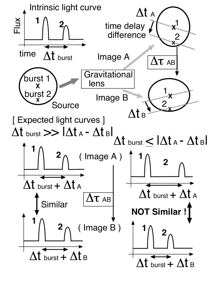
Figure 1: Schematic view of the finite-source size effect for time delay between gravitationally-lensed, split quasar image (see section 2).

The basic idea that we wish to present in this $letter$ is schematically illustrated in figure 1. Suppose the situation that a quasar is macrolensed by lensing objects so that its image is split into two (or more) images. The angular separation between these images is large enough to observe individually, say apparent angular separation is $\lower 2.15277pt\hbox{$\;\buildrel>\over{\sim}\;$}1~{}{\rm arcsec}$. If we observe such quasar images, we will realize the intrinsic variabilities of quasar in each image as in the case of an ordinary, not gravitationally lensed quasar (e.g., recent optical monitoring results are shown in Sirola et al. 1998). Because of the macrolensing effect, generally, the variabilities in such a quasar are not observed in both images at the same time. There is a time delay between these quasar images caused by a light path difference from the light path without lensing objects which originates from gravitational lens effect (e.g., see Schneider, Ehlers, & Falco 1992, hereafter SEF). These facts are nicely demonstrated by K97.

However, previous studies related to the time delay caused by gravitational lensing were not so much concerned with the source of variabilities, and the source of variabilities was treated as a point source. This treatment is reasonable, if the whole source size is negligibly small compared with the typical scale length over which a time delay changes. In contrast, actually, we only know that the source of quasar variabilities is smaller than the limit of the observational resolution, say $\lower 2.15277pt\hbox{$\;\buildrel<\over{\sim}\;$}1~{}{\rm arcsec}$ (e.g., in the case of HST observations, $\sim 0.1~{}{\rm arcsec}$), and we do not know whether the whole source size is small or large compared with the scale length over which a time delay changes. Therefore, first, we should try to consider the effect of a finite source size on the expected observed light curve in quasar images.

Then, if we include such an effect, what do we expect to see ? The answer is easily understood by figure 1. For simplicity, I consider only two images (image A and B) of the lensed quasar, and the source exhibit only two bursts (“burst 1” and “burst 2”, they occur in this order on the source plane) with some time interval ($\Delta t_{\rm burst}$). The origin and separation of such bursts are not specified, we assume that these two bursts are not physically correlated, in other words they appear randomly. Additionally, we set a time delay difference between the position of the “burst 1” and the “burst 2” on image A as $\Delta t_{\rm A}$ and that on image B as $\Delta t_{\rm B}$.

In the case of $\Delta t_{\rm burst}\gg|\Delta t_{\rm A}-\Delta t_{\rm B}|$, light curves of two images show apparently very similar feature, instead of its time delay at the very center. Although the shape of light curves is altered from intrinsic one by the effect of finite source size as is depicted in lower left part of figure 1, we can easily identify these two light curves are intrinsically the same one. Thus, we are able to obtain a robust time delay between two images.

On the other hands, in the case of $\Delta t_{\rm burst}\lower 2.15277pt\hbox{$\;\buildrel<\over{\sim}\;$}|\Delta t_{\rm A}-\Delta t_{\rm B}|$, a previous fact does not hold any more. In this case, time interval between two bursts is significantly modified by the effect of its apparently large time delay difference ($|\Delta t_{\rm A}-\Delta t_{\rm B}|$). In such a situation, we can no longer conclude that light curves from two images have the same origin, even if we include an effect of time delay for the case of point source. We may seek for the reason for this to microlensing or something exotic. In other words, there will be no good correlation between light curves of two images. This is a serious problem not only to determine time delay or $H_{\rm 0}$ but also to construct a quasar structure, to determine the origin of variabilities, or some other problems.

Here, I will make a simple estimate of time delay difference between different parts of the source, i.e., the effect of a finite source. In this estimate, I define ${\bf\beta}$,${\bf\theta_{\rm A}}$, ${\bf\theta_{\rm B}}$ as angular positions of the source center and those of the centers of two images. Therefore, ${\bf\theta_{\rm A}}$ and ${\bf\theta_{\rm B}}$ are the solutions of well-known lens equation (e.g., SEF),

$${\bf\beta}={\bf\theta}-{\bf\alpha}({\bf\theta}),$$ (1)

where, ${\bf\alpha}$ is a bending angle caused by intervening lens object(s), i.e., gravitational lens effect. Furthermore, time delay from un-lensed light path ($\tau$) in the case of the image position is ${\bf\theta}$ and the source position is ${\bf\beta}$ is written as

$$\tau=\frac{(1+z_{\rm ol})}{2c}{\cal D}\left|{\bf\theta}-{\bf\beta}\right|^{2}-\frac{(1+z_{\rm ol})}{c^{3}}\Psi({\bf\theta}).$$ (2)

Here, $z_{\rm ol}$ is redshift from observer to lens, ${\cal D}$ is effective lens distance that by using angular diameter distance from observer to lens ($D_{\rm ol}$), from observer to source ($D_{\rm os}$), and from lens to source ($D_{\rm ls}$), written as ${\cal D}=D_{\rm ol}D_{\rm os}/D_{\rm ls}$, and $\Psi$ is so-called “effective lens potential” (e.g., SEF). Insert each image position into equation (2) and subtract one equation from the other, we obtain the well-known time delay expression between images A and B ($\Delta\tau_{\rm AB}$),

$$\Delta\tau_{\rm AB}({\bf\beta})=\frac{(1+z_{\rm ol})}{2c}{\cal D}\left(\left|{\bf\theta_{\rm A}}-{\bf\beta}\right|^{2}-\left|{\bf\theta_{\rm B}}-{\bf\beta}\right|^{2}\right)-\frac{(1+z_{\rm ol})}{c^{3}}\{\Psi({\bf\theta_{\rm A}})-\Psi({\bf\theta_{\rm B}})\}.$$ (3)

Additionally, if we assume the position that is offset by $d{\bf\beta}$ from the center of the source and write $d{\bf\theta_{\rm A}}$ and $d{\bf\theta_{\rm B}}$ as image positions from the center of the image, these variables should fulfill the lens equation (1) again, i.e.,

$$({\bf\beta}+d{\bf\beta})=({\bf\theta}_{i}+d{\bf\theta}_{i})-{\bf\alpha}({\bf\theta}_{i}+d{\bf\theta}_{i}),~{}~{}~{}(i={\rm A~{}or~{}B})$$ (4)

or, subtracting this from equation (1) and adopt Taylor expansion to $\alpha$, we obtain another expression of equation (4), $d{\bf\beta}=d{\bf\theta}_{i}-\nabla_{\rm\theta}{\bf\alpha}({\bf\theta}_{i})d{\bf\theta}_{i}+\cdots$.

Subtracting $\Delta\tau_{\rm AB}({\bf\beta})$ from $\Delta\tau_{\rm AB}({\bf\beta}+d{\bf\beta})$, c.f., equation (3), and using equation (1) and equation (4), we are able to obtain the time delay difference between the center of source and the other position offset by $d{\bf\beta}$ from the center of the source ($\delta\tau_{\rm AB}=\Delta\tau_{\rm AB}({\bf\beta}+d{\bf\beta})-\Delta\tau_{\rm AB}({\bf\beta})$) on the source plane.

Moreover, by definition of effective lens potential, bending angle ${\bf\alpha}$ is related to the ${\bf\theta}$ through the derivative of effective lens potential $\Psi({\bf\theta})$ as $\nabla_{\bf\theta}\Psi({\bf\theta})/{\cal D}c^{2}={\bf\alpha}({\bf\theta})$. Since we are considering the origin of quasar variabilities, the source size is $\sim~{}{\rm kpc}$ at most and the distance from observer is typical cosmological scale $\sim 1~{}{\rm Gpc}$. Thus, its apparent angular size is $\sim~{}{\rm kpc}/1{\rm Gpc}=10^{-6}~{}{\rm rad}$. This seems to be small compared with image separation and the scale of bending angles which is typically a few arcsec. For $\delta\tau_{\rm AB}$, accordingly, we can adopt a Taylor expansion to ${\bf\alpha}$ and $\Psi$, neglect the higher terms than first order assuming $d{\bf\beta}\ll{\bf\beta}$ and $d{\bf\theta}_{i}\ll{\bf\theta}_{i}$. After using some algebra and putting $R$ as actual off-centered distance on the source plane, i.e., $R=|d{\bf\beta}|\cdot D_{\rm os}$, we are able to evaluate time delay difference as follows,

$$\delta\tau_{\rm AB} \simeq \frac{(1+z_{\rm ol})}{2c}{\cal D}\{2{\bf\alpha}({\bf\theta_{\rm A}})\nabla_{\bf\theta}{\bf\alpha}({\bf\theta_{\rm A}})d{\bf\theta_{\rm A}}-2{\bf\alpha}({\bf\theta_{\rm B}})\nabla_{\bf\theta}{\bf\alpha}({\bf\theta_{\rm B}})d{\bf\theta_{\rm B}}\}$$ (5)

$$-\frac{(1+z_{\rm ol})}{c^{3}}\{\nabla_{\bf\theta}\Psi({\bf\theta_{\rm A}})d{\bf\theta_{\rm A}}-\nabla_{\bf\theta}\Psi({\bf\theta_{\rm B}})d{\bf\theta_{\rm B}}\}$$

$$= \frac{(1+z_{\rm ol})}{c}{\cal D}\left[\{\nabla_{\rm\theta}{\bf\alpha}({\bf\theta_{\rm A}})-1\}{\bf\alpha}({\bf\theta_{\rm A}})d{\bf\theta_{\rm A}}-\{\nabla_{\rm\theta}{\bf\alpha}({\bf\theta_{\rm B}})-1\}{\bf\alpha}({\bf\theta_{\rm B}})d{\bf\theta_{\rm B}}\right]$$

$$\sim \frac{(1+z_{\rm ol})}{c}{\cal D}\left|\left({\bf\theta_{\rm B}}-{\bf\theta_{\rm A}}\right)\cdot d{\bf\beta}\right|$$

$$\sim 12\left(\frac{1+z_{\rm ol}}{2}\right)\left(\frac{D_{\rm ol}}{D_{\rm ls}}\right)\left(\frac{|{\bf\theta_{\rm B}}-{\bf\theta_{\rm A}}|}{1{\arcsec}}\right)\left(\frac{R}{1~{}{\rm kpc}}\right){\rm day}$$ (6)

This one-dimensional evaluation is somewhat overestimated, however, for the calculations above, we did not use any restriction about lens model, and equation (6) seems to be appropriate for any lens models and lensed systems except in some special situations, e.g., in the vicinity of caustics (or critical curves).

Consequently, considering the fact that quasar optical intrinsic variabilities have timescale ${\rm day}\sim{\rm month}$, equation (6) indicates that correlation between light curves of two images shown, in worst cases, will disappear, if the origin of quasar variabilities is extended over $\sim 1~{}{\rm kpc}$, i.e., maximum off-centered burst occurs at $\sim 1~{}{\rm kpc}$ from the center of quasar.

3 EXAMPLES OF Q0957+561

Finally, we will show some impressive result for the case of Q0957+561 which is the first detected lensed quasar by Walsh, Carswell, & Weymann, (1979).

To demonstrate how the extended source effect works on the time delay determination in an actual lensed quasar, here, I will present simulation results of Q0957+561 as one example. Using equation (6), we are able to estimate a time delay difference between same source positions at different lensed images. In this case, as is well known, if we use $z_{\rm ol}\simeq 0.36$, $z_{\rm os}\simeq 1.41$, $|\theta_{\rm B}-\theta_{\rm A}|\sim 6{\arcsec}$ (e.g., GN) and assumed that $H_{\rm 0}\sim 60{\rm km~{}s^{-1}~{}Mpc^{-1}}$, we will obtain $\delta\tau_{\rm AB}\sim 50~{}{\rm day}$ for the source with a size of $1~{}{\rm kpc}$ !

Furthermore, to obtain more realistic results, we used isothermal SPLS galaxy with compact core as an example of lens model for Q0957+561 (details are shown in GN), adopted parameters listed in table 7 in GN as “isothermal” SPLS and calculated time delay difference between images center and off-centered part of images ($\delta\tau_{\rm AB}$). For this calculation, we set $\Omega=1.0$ for simplicity and took on convergence $\kappa\simeq 0.22$ and $H_{\rm 0}\simeq 64~{}{\rm km~{}s^{-1}~{}Mpc^{-1}}$ to reproduce the observed time delay following K97. The resultant time delay contours compared with the image centers on the source plane are depicted in figure 2. On image A (left panel), a gradient of the contour is almost in the negative y-direction, although that of image B (right panel, this time delay advanced $\sim 417{\rm day}$ ) is almost in the positive y-direction. Additionally, time difference between the same position on the source reaches order of $\sim{\rm months}$ for the case of the source with a $\sim{\rm kpc}$ size, therefore, we expect disappearance of correlations between the light curves of image A and that of image B. Here, from equation (5), we can easily understand why do the contour lines show almost straight and perpendicular to y-direction. Product of $({\bf\theta_{\rm A}}-{\bf\theta_{\rm B}})$ and $d{\bf\beta}$ in equation (5) means that time delay difference determined mostly by the element which parallel to $({\bf\theta_{\rm A}}-{\bf\theta_{\rm B}})$ of displacement $d{\bf\beta}$. Therefore, the time delay difference significantly alters along the $({\bf\theta_{\rm A}}-{\bf\theta_{\rm B}})$ direction and almost constant along the perpendicular direction.

Moreover, we simulated expected light curves of variabilities in both quasar images using superposition of simple bursts with triangled shape and duration of $\sim 10$ days which are randomly distributed in time, in space, and in amplitude. For the whole source size, I consider three cases, $1~{}{\rm kpc}$, $100~{}{\rm pc}$ and $10~{}{\rm pc}$. Using the same procedure to produce figure 2, we calculated time delay from the center of image A over both images, randomly produce bursts, sum up all bursts and finally obtain expected light curves as presented in figure 3. “Residual light curves” produced by subtracting properly-shifted light curve of image B from that of image A, are also shown in the figure. In the case of the smallest source, $R=10~{}{\rm pc}$, and still in the case of middle source size, $R=100~{}{\rm pc}$, we can easily recognize the coherent pattern in the light curves of images A and B but with time delay of $\sim 417~{}{\rm days}$ advanced light curve of image B. Time delay between two image centers is able to be determined fairly well. However, in the case of largest source, $R=1~{}{\rm kpc}$, it seems no correlation between two light curves even if we already know the time delay between two image centers, and we may misunderstand that the variabilities did not originate in source itself ! This feature is far from the observed properties that the time delay between two images is determined easily even if we fit them by eyes. Therefore, I conclude that the size of source that is origin of quasar variabilities should be smaller than $100~{}{\rm pc}$, namely, maximum acceptable size is order of $\sim 10~{}{\rm pc}$ from this simple simulation.

4 DISCUSSIONS AND COMMENTS

As we examined, if we include the finite source-size effect to the time delay determination from quasar variabilities, correlation between expected light curves of each lensed image will disappear in the case of the size is sufficiently large, say $\sim 1{\rm kpc}$. Using this fact, we can limit the size of the region where quasar variabilities are produced, from the correlation between light curves of multiple lensed quasar images. Furthermore, since the size of the origin of intrinsic quasar variability reflects a physical origin of the variabilities, we can also determine the origin of the variabilities, e.g., whether it is disk instability (Kawaguchi et al. 1998) or star burst (Aretxaga, Cid Fernandes, & Terlevich, 1996). Particularly, in the case of Q0957+561, the origin of variabilities has a size smaller than $100~{}{\rm pc}$. This value is consistent with disk instability model, because of its small size ($\sim 0.01{\rm pc}$ for $1000$ Schwarzschild radius accretion disk surrounding $10^{8}M_{\odot}$ supermassive black hole). Starburst model can be rejected, since starburst region is $100~{}{\rm pc}\sim 1~{}{\rm kpc}$. Hence, for the origin of intrinsic quasar variabilities, the disk instability model is more preferable, as was indicated by Kawaguchi et al. (1998) already. To draw this conclusion more critically, we should do this study more precisely in future.

Additionally, the fact that a larger source size tends to reduce a good correlation between the light curves of each image provides an answer to the question why time delay determination from radio flux gave a wrong answer except recent works, e.g., Haarsma et al (1999). Generally, radio emitting region is believed to have a larger size than that of optical photon because of the existence of large radio lobe and/or jet component, and the effect we have shown in this $letter$ may be significant. Thus, robust determination of the time delay seems to be difficult.

If such a effect is significant in the well-known lensed quasar Q2237+0305, microlens interpretation of individual variabilities (e.g., see Irwin et al. 1989) will be rejected. Fortunately, however, this may not be the case because for this source, caused by its quite nice symmetry of lensed image, the effect seems not to be so significant and intrinsic variabilities will be expected to appear in every images with good correlations.

If we develop this technique furthermore, and adapted to another multiply-imaged lensed quasar, we will determine the size of the most interesting part in quasar.

Figure 2: Contour of time delay difference at image A (left panel) and image B (right panel) compared with their own center. The y-axis positive to north same as GN and the axis is almost parallel to the ${\bf\theta_{\rm A}}-{\bf\theta_{\rm B}}$ direction. Source center is shown by filled circle at the center of each figures and long-dashed circles present a circle with a diameter of $1~{}{\rm kpc}$, $300~{}{\rm pc}$, and $100~{}{\rm pc}$ from outer one to inner one, respectively. The time delay contours of leading parts (solid lines), preceding parts (dotted lines), and no time delay from the center parts (dashed lines) are presented. Concrete values are also shown in the figures.

Figure 3: Simulated light curves (upper one of each panel) of image A (solid curve) and B (dashed curve), and its residual light curves (lower one) for some different source size. Numeric values on the horizontal line are fluxes normalized by a standard deviation of light curve of image A ($\sigma_{\rm A}$). The whole source sizes are $10~{}{\rm pc}$ (upper panel), $100~{}{\rm pc}$ (middle panel), and $1~{}{\rm kpc}$ (lower panel). The curves are arbitrary shifted in the vertical direction. A light curve in dotted box of image A and B should be the same in the case of point-source treatment.

References

- (1) Aretxaga, I., Cid Fernandes, R., & Terlevich, R.J. 1997, M.N.R.A.S., 286, 271
- (2) Grogin, N.A., & Narayan, R. 1996, ApJ, 464, 92; Erratum 473, 570 (GN)
- (3) Haarsma, D.B., Hewitt, J.N., Lehár, J., & Burke, B.F. 1999. ApJ, 510, 64
- (4) Irwin, M.J., Webster, R.L., Hewitt, P.C., Corrigan, R.T., & Jedrzejewski, R.I. 1989, AJ, 98, 1989
- (5) Kawaguchi, T., Mineshige, S., Umemura, M., & Turner, E.L. 1998, ApJ, 504, 671
- (6) Kundić, T., et al. 1997, ApJ, 482, 75 (K97)
- (7) Lewis, G.F., & Ibata, R.A. 1998, ApJ, 501, 478
- (8) Liebes, S. 1964, Phys. Rev., 133, B835
- (9) Mediavilla, E., et al. 1998, ApJ, 503, L27
- (10) Refsdal, S. 1964, M.N.R.A.S., 128, 295
- (11) Schneider, P., Ehlers, J., & Falco, E.E. 1992, Gravitational Lenses, 2nd ed. (New York:Springer-Verlag), p215 (SEF)
- (12) Sirola, C.J., et al. 1998, ApJ, 495, 659
- (13) Walsh, D., Carswell, R.F., & Weymann, R.J. 1979, Nat., 279, 381
- (14) Yonehara, A., Mineshige, S., Manmoto, T., Fukue, J., Umemura, M., & Turner, E.L. 1998, ApJ, 501, L41; Erratum 511, L65
- (15) Yonehara, A., Mineshige, S., Fukue, J., Umemura, M., & Turner, E.L. 1999, A&A, 343, 41