The Brera Multi-scale Wavelet (BMW) ROSAT HRI source catalog.
II: application to the HRI and first results.

Abstract

The wavelet detection algorithm (WDA) described in the accompanying paper by Lazzati et al. is made suited for a fast and efficient analysis of images taken with the High Resolution Imager (HRI) instrument on board the ROSAT satellite. An extensive testing is carried out on the detection pipeline: HRI fields with different exposure times are simulated and analysed in the same fashion as the real data. Positions are recovered with few arcsecond errors, whereas fluxes are within a factor of two from their input values in more than 90% of the cases in the deepest images. At variance with the “sliding-box” detection algorithms, the WDA provides also a reliable description of the source extension, allowing for a complete search of e.g. supernova remnant or cluster of galaxies in the HRI fields. A completeness analysis on simulated fields shows that for the deepest exposures considered ($\sim 120$ ks) a limiting flux of $\sim 3\times 10^{-15}\rm\ erg\,s^{-1}\rm\ cm^{-2}$ can be reached over the entire field of view. We test the algorithm on real HRI fields selected for their crowding and/or presence of extended or bright sources (e.g. cluster of galaxies and of stars, supernova remnants). We show that our algorithm compares favorably with other X–ray detection algorithms such as XIMAGE and EXSAS.

The analysis with the WDA of the large set of HRI data will allow to survey $\sim 400$ square degrees down to a limiting flux of $\sim 10^{-13}\rm\ erg\,s^{-1}\rm\ cm^{-2}$ and $\sim 0.3$ square degrees down to $\sim 3\times 10^{-15}\rm\ erg\,s^{-1}\rm\ cm^{-2}$. A complete catalog will result from our analysis: it will consist of the Brera Multi-scale Wavelet Bright Source Catalog (BMW-BSC) with sources detected with a significance $\gtrsim 4.5\,\sigma$ and of the Faint Source Catalog (BMW-FSC) with sources at $\gtrsim 3.5\,\sigma$. A conservative estimate based on the extragalactic $\log(N)-\log(S)$ indicates that at least 16000 sources will be revealed in the complete analysis of the whole HRI dataset.

1. INTRODUCTION

The next generation of X–ray instruments, such as AXAF or XMM, will provide deep X–ray images with very high source density (up to $1000/{\rm deg{{}^{2}}}$). To fully exploit the scientific content of these data, new and more refined detection techniques have to be considered. Algorithms based on the wavelet transform provide one of the best analysis tools, which has been already used in astronomy over the last decade (Coupinot et al. 1992; Slezak et al. 1993, 1994; Rosati 1995; Rosati et al. 1995; Grebenev et al. 1995; Damiani et al. 1997a; Vikhlinin et al. 1998).

We have fully implemented a Wavelet Detection Algorithm (WDA) in order to meet the confidence requirements needed to deal with a large set of data (see the accompanying paper by Lazzati el at. 1999; Paper I hereafter). Here we focus on the application of this WDA to the X–ray images taken with the High Resolution Imager (HRI) on board the ROSAT satellite, detailing the HRI-specific features of the algorithm and presenting the first results of an on-going automatic analysis on all available data.

Catalogs of X–ray sources with more than thousands of objects have been produced in the last few years (WGA: White, Giommi & Angelini 1994; ROSATSRC: Zimmermann 1994; RASS: Voges et al. 1996; ASCASIS: Gotthelf & White 1997; ROSAT Results Archive: Arida et al. 1998). These catalogs are mainly based on the Position Sensitive Proportional Counter (PSPC) on board the ROSAT satellite and have been heavily used in many research projects on different class of X–ray sources (e.g. Padovani & Giommi 1996 on blazars; Fiore et al. 1998 on quasars; Angelini, Giommi & White 1996 on X–ray variable sources; Israel 1996 on X–ray pulsars).

The most appealing feature in using the ROSAT HRI data rather than the PSPC one is provided by the sharp core of the Point Spread Function (PSF), of the order of few arcseconds FWHM on-axis. This allows to detect and disentangle sources in very crowded fields and to detect extended emission on small angular sizes. Moreover, the search for counterparts at different wavelengths will be greatly simplified by the reduced error circles. On the other hand, the ROSAT HRI instrument has a very crude spectral resolution, thus a spectral analysis can not be carried out. It is less efficient than the PSPC by a factor of $\sim 4$ (3–8 for a plausible range of incident spectra) and, finally, it has a higher instrumental background. More details on the performances of the HRI are given in Section 2. In Section 3 we describe the application of the WDA to HRI data. Section 4 is devoted to the illustration of the simulations carried out to test the detection pipeline. In Section 5 we show the WDA results on “difficult” fields (e.g. very crowded fields, clusters of galaxies and of stars, supernova remnants). In Section 6 we summarise our conclusions.

2. HIGH RESOLUTION IMAGER

The HRI on board the ROSAT satellite is a position sensitive detector based on microchannel plates, that reveals single X–ray photons and determines their positions and arrival times (for more details see David et al. 1998). The ROSAT HRI is very similar to the Einstein HRI. The nominal pixel size of $0.5^{\prime\prime}$ has been reduced to $0.4986^{\prime\prime}$ after detailed observations on the Lockman hole field (Hasinger et al. 1998). The HRI field of view is given by the intersection of the circular detector and a square readout, resulting in octagon-like shape with $\sim 19^{\prime}$ radius. The HRI PSF on-axis is $\sim 5^{\prime\prime}$ FWHM, well modeled with two Gaussians plus an exponential function. Due to random errors in the aspect solution however, images may be occasionally ellipsoidal and the PSF parameters may vary up to $\sim 15\%$. The HRI PSF degrades rapidly for off-axis angles beyond $\sim 5^{\prime}$ whereas it becomes very asymmetric beyond $\sim 12^{\prime}$. The PSF off-axis is not known with good accuracy and, up to now, only a description of the Gaussian widths with the off-axis angle has been published (David et al. 1998). Here we adopted a different approach. We make use of a ray-tracing simulator in order to extrapolate the well known on-axis PSF to any off-axis angle; in this way we get rid of aspect solution and photon statistic problems (see Appendix A for more detail).

The on-axis effective area is 83 cm² at 1 keV, while the vignetting is less than 10% within $10^{\prime}$ at all energies. The effective area has not varied significantly since launch. Systematic uncertainties amount to $\lesssim 3\%$.

The HRI covers an energy range of 0.1–2.4 keV, divided in 16 Pulse Height Analyzer (PHA), which provide very crude spectral information. Hardness ratios can give some qualitative information, but the gain variations lead to the definition of the PHA boundaries on a case by case basis (Prestwich et al. 1998).

The HRI background is made of several components: the internal background due to the residual radioactivity of the detector (1–2 cts s^-1), the externally-induced background from charged particles (1–10 cts s^-1) and the X–ray background (0.5–2 cts s^-1). The background is the highest in the first few (1–3) PHA channels and it is dominated by the first two components. As shown by sky calibration sources, most of the source photons instead fall between PHA channel 3 and 8, approximately (David et al. 1998).

3. Wavelet Detection Algorithm for the HRI

The analysis and source detection of HRI images takes place in several steps, here we briefly describe the analysis of HRI images (see Fig. 1). The detection algorithm is presented and described in detail in Paper I (see also Fig. 1 therein).

3.1. Image extraction

Due to computer limitations it is not efficient to analyse the entire HRI image in one single step, preserving the original angular resolution (it would result in a $\sim 5000\times 5000$ pixels image). In order to maintain the superb HRI angular resolution, we analyse the images in more steps. We extract a $512\times 512$ pixels image rebinned by a factor of 1 (pixel size $0.5^{\prime\prime}$), as well as concentric images rebinned by a factor of 3 (pixel size $1.5^{\prime\prime}$), 6 (pixel size $3^{\prime\prime}$) and 10 (whole image with pixel size $5^{\prime\prime}$), respectively. These images are extracted from the relevant event files using the XIMAGE program (Giommi et al. 1992). Each image is then analysed separately.

3.2. Background estimate

For each image a mean background value is estimated using a $\sigma-$clipping algorithm (see Paper I): the mean and standard deviation of an image are calculated and pixels at more than $3\,\sigma$ above the mean value are discarded. The procedure works iteratively, rebinning the image and discarding outstanding pixels. We carried out various simulations on HRI fields and found that even in crowded fields the background value is recovered within $\sim 10\%$. We checked these values using the background estimator within XIMAGE obtaining the same results and accuracy.

3.3. Exposure map

X–ray mirrors, like optical mirrors, are vignetted. This generates non-flat fields where the detection of X–ray sources is made difficult by the second-order derivative of the background component (the adopted WT is insensitive to constant or first-order background components, see Paper I). In addition to this component, there may be obscuring structures (like the ROSAT PSPC rib) or hot regions in the detector (like in the EXOSAT Channel Multiplier Array) or real sky background variations (e.g. in the presence of extended sources). For these reasons it is usually better to perform the source search on top of a background map, rather than on a flat background. In the particular case of the ROSAT HRI, this allows us to search also for sources which lie in the edge region, where the detector efficiency rapidly drops to zero. In this case the linearity of the wavelet transform helps us: since an image can be thought as the sum of a background component plus the sources, the transform of the source component can be obtained subtracting the transform of the background map from that of the whole image. Background maps are provided together with the relevant data (as in the case of ROSAT PSPC) or can be generated through dedicated software (as the ESAS software for both ROSAT PSPC and HRI instruments; Snowden et al. 1994).

A different approach is to properly smooth the source image, filtering out the brightest sources, and using this image as the background map (Vikhlinin et al. 1995b; Damiani et al. 1997a). This approach is also useful in the presence of extended emission which cannot be modeled analytically (e.g. supernova remnants) even if the smearing of extended and faint sources tends to reduce source significance and hence the completeness of the catalog.

At variance with the ROSAT PSPC, the HRI background is dominated by the unvignetted particle background. In order to minimise the impact of this background and more generally to increase the signal-to-noise (S/N) ratio of X–ray sources, we restrict our analysis to PHA 2–9 (see also David et al. 1998; Hasinger et al. 1998). This range reduces the detector background by about 40% with a minimum loss of cosmic X–ray photons ($\lesssim 10\%$; David et al. 1998). To build the exposure map we adopt the ESAS software (Snowden 1994) that makes use of the bright Earth and dark Earth data sets to produce a vignetted sky background map and a background detector map, respectively. The mean image background, as estimated with the $\sigma-$clipping algorithm (see above), is used to normalise the sky background map provided by the ESAS software. The total background map is then obtained by summing up the detector and sky maps. The ESAS maps are produced at rebin 10 (pixel scale $5^{\prime\prime}$), thus we interpolate them to obtain the maps at rebin 1, 3 and 6. These three maps are then smoothed with a Gaussian filter with a size twice the mean PSF, in order to get rid of interpolation inhomogeneities.

3.4. Image analysis

The four images and relative exposure maps are searched for significant enhancements using the WDA. On the first three images the detection is performed within an annulus of 255 pixels excluding a border at the detector edge of the local PSF width ($\sim 5^{\prime\prime}$, $\sim 7^{\prime\prime}$ and $\sim 12^{\prime\prime}$ at rebin 1, 3 and 6, respectively). This strategy has been adopted in order to preserve the original circular symmetry of the image and to avoid the occurrence of azimuthally dependent detection thresholds. In fact, detecting sources on the whole $512\times 512$ pixels image would result in a bias at the corners between 255 pixels (i.e. the image radius) and $255\,\sqrt{2}$ (i.e. half the square diagonal). Sources in the region left over are recovered at the successive rebin. At rebin 10 the whole image is handled.

The detection threshold choice has deep impact on the characteristics of the catalog to be produced. The use for statistical purposes (such as $\log(N)-\log(S)$) of the catalog requires a high threshold (i.e. low contamination), whereas a low threshold is needed for the detection of a large number of sources, even if plagued by higher contamination. For these aims, we consider two different detection thresholds: a contamination of 0.1 spurious source per field is allowed for the Brera Multi-scale Wavelet Bright Source Catalog (BMW-BSC); a contamination of 1 spurious source per field is used for the Faint Source Catalog (BMW-FSC). The equivalent thresholds applied to BMW-BSC and BMW-FSC correspond to a source significance of $\sim 4.5\,\sigma$ and $\sim 3.5\,\sigma$, respectively. These detection thresholds are given for each field as a whole and must therefore be shared among the four rebinned images, holding the relative contamination constant over the full HRI field. The detection threshold for each rebinned image cannot be just one forth of the whole threshold (e.g. 0.25 in the case of 1 spurious source per field), due to the different area analysed at each rebin. A proper weighting factor is given by the ratio between the analysed area and the mean PSF width at each rebin.

3.5. Corrections

The HRI data are pre-processed with the ROSAT Standard Analysis System (Voges 1992) which provides images corrected for detector non-linearities and attitude control. We also apply the vignetting and gain correction, deriving them from the final exposure map. A deadtime correction in the case of bright sources is also applied (David et al. 1998).

To these we have to add other small corrections related to the detection algorithm we use. To fit the sources in the wavelet space we approximate the PSF with a single Gaussian. However, the PSF has an extended tail and becomes increasingly asymmetric with the off-axis angle, thus we systematically loose counts. Since the HRI PSF is not well known at large off-axis angles, we performed ray-tracing simulations all over the field of view (see Appendix A). We then fit these ray-tracing simulated images with the WDA and derived the PSF correction needed to obtain the real flux (the PSF correction is a common characteristic of all detection algorithms). This PSF correction depends on the off-axis angles and varies from $\sim 18\%$ for sources at off-axis angles $\theta\lesssim 2^{\prime}$ (i.e for all sources in the image at rebin 1) to $\sim 13\%$ for $6^{\prime}\lesssim\theta\lesssim 13^{\prime}$ (i.e. at rebin 6; see Table 1). At rebin 10 the PSF degradation makes this correction a steep function of the off-axis angle (see Table 1). The reduction of the PSF correction with the off-axis angle is likely due to the vanishing importance of the second Gaussian in the PSF.

The HRI PSF becomes increasingly asymmetric with the off-axis angle, developing a bright spot (the center of which coincides with the source position) on top of an extended emission (as shown also by our ray-tracing simulations). The center of this extended emission is shifted by a few arcsec from the spot in the direction opposed to the field center. Fitting the counts distribution of an X–ray source with a Gaussian, the WDA finds its position in between the bright spot and the center of the extended emission (even if much nearer to the spot). In order to correct for this (small) effect which is mainly due to the larger support of the wavelet functions, we selected 4 HRI exposures with a large number of sources (Trapezium ROR 200500; P1905 ROR 200006; IC348 ROR 201674 and NGC2547 ROR 202298). We first performed a boresight correction on the central sources, then we selected X–ray sources associated with Guide Star Catalogue objects within $10^{\prime\prime}$. We measured the distance between the X–ray sources and the optical counterparts as a function of the off-axis angle. Even if a (small) number of spurious identifications can take place, we note that a systematic effect is clearly evident in Fig. 2. In particular the radial shifts are linearly correlated with the off-axis angle and the best fit line provides a correction of about $7^{\prime\prime}$ for a source at $18^{\prime}$ off-axis (this value includes also the $\sim 3^{\prime\prime}$ correction for the smaller pixel size, cf. Section 2). The scatter in the source off-sets is rather large so we decided to conservatively compute the $3\,\sigma$ uncertainty on the best fit line by individuating the region that includes the 99.7% of sources (cf. Fig. 2). This is achieved by considering the two dashed lines in Fig. 2. The derived error is of about $7^{\prime\prime}$ for a source at $18^{\prime}$ off-axis at a $3\,\sigma$ level. This shift error has been summed in quadrature to the position error derived from the fit and it provides the total error for the sources in our catalog.

We point out that this result should not be regarded as a different HRI plate scale as reported in David et al. 1998 and Hasinger et al. 1998. The radial shift found in this analysis is mainly caused by the larger support of the wavelet functions that probe the source PSF on a larger scale than the sliding box techniques.

3.6. Creation of the catalog

For each observation we derive a catalog of sources with position, count rate, extension along with the relative errors, as well as ancillary information about the observation itself and source fitting. The count rate has been computed by fitting the image transform at all scales simultaneously in the wavelet space (see Paper I). We provide also a second count rate estimate following the standard approach of counting the source photons, however this method fails e.g. in the case of crowded fields or extended emission. The counts to flux conversion factor is determined based on a Crab spectrum. In the case of high latitude fields ($|b|>30^{\circ}$) the galactic column density is assumed, whereas for lower latitude fields we consider either a null column density and the galactic value, therefore providing a range of fluxes. Together with the information relative to the X–ray data, we cross correlate the detected sources with databases at different wavelengths to give a first identification.

One of the most interesting feature of the wavelet analysis is the possibility of characterising the source extension, however this cannot be assessed simply by comparing the source width ($\sigma$, as derived by the fitting procedure) with the HRI PSF (e.g. as derived by the ray-tracing simulator) at a given off-axis angle, due to the energy dependence of the PSF width as well as to errors in the aspect reconstruction (near on-axis). Thus, to assess the source extension, we considered a version of the catalog consisting of sources detected in the observations that have a star(s) as a target (ROR number beginning with 2). We considered 756 HRI fields and we detected 6013 sources in the BMW-BSC catalog (Fig. 3). The distribution of source extensions has been divided into bins of $1^{\prime}$ each, as a function of the source off-axis angles. In each $1^{\prime}$ bin, we applied a $\sigma-$clipping algorithm on the source extension: the mean and standard deviation in each bin are calculated and sources with widths at more than $3\,\sigma$ above the mean value are discarded. This method iteratively discards truly extended sources and provides the mean value of the source extension ($\sigma$) for each bin along with its error. We then determine the $3\,\sigma$ dispersion on the mean extension for each bin. The mean value plus the $3\,\sigma$ dispersion provide the line demarking source extension (cf. the dashed line in Fig. 3; see also Rosati et al. 1995). We conservatively classify a source as extended if its error on the extension parameter is such that it lays more than $2\,\sigma$ from this limit (see Fig. 3). Combining this threshold with the $3\,\sigma$ on the intrinsic dispersion we obtain a $\sim 4.5\,\sigma$ confidence level for the extension classification. 254 sources have been classified as extended, which makes up $\sim 4\%$ of the total. Note that no source has been classified as extended on-axis, as should be expected being stars the targets.

A word of caution has to be spent for the flux estimate of extended sources. The source flux is computed by fitting a Gaussian to the surface brightness profile and, in many cases, this provides a poor approximation. Therefore, fluxes of extended sources are usually underestimated. A solution in the case of extended sources with well-defined surface brightness profiles (i.e. clusters of galaxies) has been presented by Vikhlinin et al. 1998.

4. SIMULATIONS

The WDA presented in paper I has provided very good results on ideal fields, with flat background, Gaussian sources and no crowding. To test the whole pipeline also on realistic images, we simulated sets of HRI observations using real instrumental background maps generated with the Snowden’s software and superposing X–ray sources following the soft X–ray $\log(N)-\log(S)$ by Hasinger et al. 1993 (see also Vikhlinin et al. 1995b). We took the exposure map of one of the longest observations in the ROSAT public archive (NGC 6633 - ROR 202056a01 - $\sim 120$ ks), and superpose X–ray sources down to a flux of $\sim 5\times 10^{-16}\rm\ erg\,s^{-1}\rm\ cm^{-2}$ (a conversion factor of $1\,{\rm cts\,s^{-1}}=1.71\times 10^{-11}\rm\ erg\,s^{-1}\rm\ cm^{-2}$ in the 0.5–2.0 keV energy band has been adopted; Hasinger et al. 1998). Each simulated image contains 500 sources, the faintest of which have $\sim 3$ counts and enhance the sky background being well below the detection threshold. The sources were distributed homogeneously all over the field of view and the appropriate PSF obtained with the ray-tracing simulator was used to spread their photons. A total of 100 fields were simulated and analysed in the same automatic fashion as the real data. Every detected output source has been identified with a simulated input source within the $3\,\sigma$ error box.

These simulations allow to probe the WDA algorithm behaviour on “real” HRI fields, revealing the presence and the influence of biases and selection effects (e.g. Hasinger et al. 1993; Vikhlinin et al. 1995a). The great majority (more than 90%) of source fluxes are recovered within a factor of 2 of their input values. The tail of the counts distribution starts enlarging at $\sim 120$ counts over the entire field of view (i.e. $\sim 2\times 10^{-14}\rm\ erg\,s^{-1}\rm\ cm^{-2}$, see Fig. 4). This effect is produced by the combination of source confusion (e.g. Hasinger et al. 1998) and the bias in the source intensity determination extensively discussed by Vikhlinin et al. 1995a. The latter occurs due to the preferential selection of sources coincident with positive background fluctuations, near the detection threshold and it is more severe for surveys with low S/N ratios. Comparing the results on the simulated HRI fields with the ones with equally spaced sources discussed in Paper I (cf. Figure 5), we conclude that source confusion is more important. We remark that source confusion affects only a small fraction of the sources ($\lower 2.15277pt\hbox{$\;\buildrel<\over{\sim}\;$}10\%$). If, in fact, we quantify the confusion following Hasinger et al. 1998 (cf. Equation 5 therein), we are far below the strong confusion regime.

In order to explore the influence of biases and selection effects we simulated also 50 fields at five different exposure times (1, 7, 15, 30 and 60 ks) each. Rather than adopting the Hasinger’s $\log(N)-\log(S)$ distribution (which implies about 3 sources per field at 7 ks), we considered in these cases a simpler one, i.e. a power law $\log(N)-\log(S)$ with an index of –2.5 and with arbitrary normalisation set to have about 200 sources per frame. This approach has been adopted in order to reduce the number of simulations and therefore computing time (which is mainly spent in the calculation of the image and background transforms) and it results in a more stringent test on the WDA due to the heavier crowding. The relative completeness functions are plotted in Fig. 6. As one can see the 95% limiting flux moves from $\sim 4\times 10^{-13}\rm\ erg\,s^{-1}\rm\ cm^{-2}$ to $\sim 3\times 10^{-14}\rm\ erg\,s^{-1}\rm\ cm^{-2}$ (see Fig. 5). These numbers refer to a completeness achieved over the full field of view. Lower values can be obtained reducing the area of interest. The total number of counts needed to achieve the 95% completeness level as a function of the exposure time can be well approximated by a constant plus a square root function (see Fig. 6).

4.1. General properties of the survey

The sensitivity of the HRI instrument is not uniform over the field of view but decreases rapidly with the off-axis angle as a consequence of the PSF broadening and mirror vignetting. For this reason the surveyed region at a given limiting flux should not necessarily coincide with the HRI detector area but is in general a smaller circular area. We compute the sky coverage of a single observation by calculating the detection thresholds over the entire field of view. With the help of the ray-tracing program we simulated sources from $0^{\prime}$ to $18^{\prime}$ off-axis with a $1^{\prime}$ step. We then properly rebin these simulated images and calculate the minimum number of counts needed to reveal the source at the selected off-axis angle as a function of the image background. A sky survey of $\sim 400$ square degrees is expected down to a limiting flux of $\sim 10^{-13}\rm\ erg\,s^{-1}\rm\ cm^{-2}$, and of 0.3 square degrees down to $\sim 3\times 10^{-15}\rm\ erg\,s^{-1}\rm\ cm^{-2}$. A preliminary and conservative estimate based on the extragalactic soft X–ray $\log(N)-\log(S)$ indicates that about 16000 sources will be revealed in the complete analysis of the whole set of HRI data (BMW-BSC). In Fig. 7 we show the differential and integral distributions of exposure times and galactic absorptions.

We also computed the $\log(N)-\log(S)$ distribution based on the dataset of 120 ks simulations (see above). The recovered distribution is complete down to a flux of $\sim 10^{-14}\rm\ erg\,s^{-1}\rm\ cm^{-2}$ over the entire ($18^{\prime}$) field of view. The knowledge of the sky coverage allows us to correct for the loss of sources, enabling us to recover input $\log(N)-\log(S)$ down to a flux of $\sim 3\times 10^{-15}\rm\ erg\,s^{-1}\rm\ cm^{-2}$ (Fig. 8).

5. FIRST RESULTS ON SELECTED HRI FIELDS

To test our HRI pipeline, we examined a sample of HRI fields (see Table 2) selected for their “difficulty” in terms of source confusion and extended emission, for which sliding box techniques face serious problems. We compare the results obtained with our WDA with the detections made with XIMAGE/XANADU (Giommi et al. 1992) and EXSAS/MIDAS (Zimmermann et al. 1993). We have to point out that the detection algorithm in XIMAGE is not optimised for the HRI so that, especially at large off-axis angles where the PSF degrades, strong sources are usually detected as multiple; on the other hand EXSAS/MIDAS has been specifically developed to deal with the ROSAT data.

We ran our WDA on these fields automatically without particular settings. For XIMAGE we set the probability threshold to $7\times 10^{-6}$ and for EXSAS the maximum likelihood (ML) to 8 but kept sources with a final ML$\,\geq 12$, which correspond to a statistical significance of $\sim 4.5\,\sigma$.

In Table 2 we report the number of sources detected with the different algorithms as well as the number of sources for each rebin image (in the case of WDA we report the number of sources for each image, rather than in a circle as described above, in order to allow the comparison). As one can see the WDA is more efficient in detecting faint sources. Even for fields where the number of sources detected with the other two algorithms is higher than for the WDA, a closer inspection reveals that this is typically due to the presence of a strong or extended source, that has been splitted into multiple sources.

To better compare the algorithms we plot in Fig. 9 the inner part of the M31 and Trapezium images: of the 59 sources detected (21 in M31 and 38 in Trapezium) at rebin 1 by our WDA, 35 (13+22) are in common with the other two algorithms, 11 (3+8) are found by WDA and EXSAS and 10 (4+6) by WDA and XIMAGE. Two sources (0+2) are found by XIMAGE and EXSAS and not by the WDA. 3 (1+2) sources are found by WDA only, 9 (5+4) by EXSAS only and 12 (0+12) by XIMAGE only. If we retain sources detected by at least two algorithms as “real” and sources with only one detection as “non-real”, we have that the WDA is characterised by the smallest number of “missed” and “spurious” sources.

6. CONCLUSIONS

The general theory underlying the WT-based algorithm we developed has been described in Paper I, together with the extensive testing we carried out. Here we focused on the application of this WDA to ROSAT HRI images, describing the HRI-dependent features, the major problems encountered (e.g. the sharp drop in the background at the detector edges and the PSF broadening with the off-axis angle) as well as the extensive testing on simulated images. The use of the Snowden’s background maps and the modeling of the HRI PSF with a ray-tracing simulator allowed us to overcome them and to perform the source search over the entire HRI field of view. In particular, we were able to optimise our WDA such that more than 90% of sources have output fluxes within a factor of two of their input values in the deepest images we simulated (120 ks). The use of a wavelet-based algorithm allows to flag extended sources in a complete catalog of X–ray sources.

The completeness functions for different exposure times have been computed with simulated images. For an exposure time of 120 ks we reach a completeness level of 95% at a limiting flux of $\sim 10^{-14}\rm\ erg\,s^{-1}\rm\ cm^{-2}$ over the full field of view. Correcting for the sky coverage the $\log(N)-\log(S)$ distribution can be extended down to $\sim 3\times 10^{-15}\rm\ erg\,s^{-1}\rm\ cm^{-2}$ over the entire field of view. The analysis with the WDA of the large set of HRI data will allow a sky survey of $\sim 400$ square degrees down to a limiting flux of $\sim 10^{-13}\rm\ erg\,s^{-1}\rm\ cm^{-2}$, and of $\sim 0.3$ square degrees down to $\sim 3\times 10^{-15}\rm\ erg\,s^{-1}\rm\ cm^{-2}$. A conservative estimate based on the extragalactic $\log(N)-\log(S)$ indicates that at least 16000 sources will be revealed in the complete analysis of the whole set of HRI data (BMW-BSC).

The WDA we developed is also tested on difficult fields and it compares favorably with other detection algorithms such as XIMAGE and EXSAS, both for what concerns the sensitivity to blended and/or weak sources and the reliability of the detected sources.

A complete and public catalog will be the outcome of our analysis: it will consist of a BMW-BSC with sources detected with a significance $\gtrsim 4.5\,\sigma$ and a fainter BMW-FSC with sources at $\gtrsim 3.5\,\sigma$. All the detected HRI sources will be characterised in flux, size and position and will be cross-correlated with other catalogs at different wavelengths (e.g. Guide Star Catalog, NRAO/VLA Sky Survey etc.), providing a first identification. The BSC can and will be used for systematic studies on different class of sources as well as for statistical studies on source number counts. These images and related information would be available through a multi-wavelength Interactive Archive via WWW developed in collaboration with BeppoSAX-Science Data Center, Palermo and Rome Observatories. The layout of a typical image is displayed in Fig. 10.

The WDA used for the analysis of HRI sources can be adapted for future X–ray missions, such as JET-X, XMM and AXAF. The application of wavelet-based detection algorithms to these new generation of X–ray missions will provide an accurate, fast and user friendly source detection software.

$$PSF(R)=\left\{\begin{array}[]{lr}A_{1}\,\exp{(-{{R^{2}}\over{2\,\sigma_{1}^{2}}})}+A_{2}\,\exp{(-{{R^{2}}\over{2\,\sigma_{2}^{2}}})}+A_{3}\,\exp{(-{R\over{\sigma_{3}}})}&{\rm for\ \theta\lesssim 3^{\prime}}\\ A_{g}\,\exp{-({{R^{2}}\over{2\,\sigma_{g}^{2}}})}+K_{1}\,(1+({R\over{r_{c}}})^{2})^{-I_{K}}&{\rm for\ \theta\gtrsim 3^{\prime}}\\ \end{array}\right.$$ (1)

where the values of the parameters can be found in Table 3.

In Fig. 11 we compare a real image of the bright white dwarf HZ 43 taken with the HRI at an off-axis angle of $15^{\prime}$ with an image simulated with the ray-tracing program. Images are normalised to have the same number of counts. We note that the ray-tracing simulation is able to reproduce the bright spot as well as the slightly offset extended halo.

Figure 1.— Block diagram of the BMW pipeline.

Figure 2.— Radial shift between the X–ray source positions and their GSC optical counterparts versus the off-axis angle. The continuous line represents the best fit to the data. Dashed lines mark a conservative $3\,\sigma$ limit to the fit (see text).

Figure 3.— Source extension ($\sigma$) versus off-axis angle for 6013 sources detected in HRI fields on stars (BMW-BSC). The dashed line marks the $3\,\sigma$ extension limit for point sources, whereas the continuous line the computed PSF. To be more conservative we consider as extended the sources lying more than $2\,\sigma$ above this line (filled squares). Crosses marks sources which lie at a significance lower than $2\,\sigma$ from this line. 254 sources have been classified as extended.

Figure 4.— Input versus output counts for detected sources in 100 simulated HRI images (120 ks). The whole field of view has been considered (left panel), whereas the results for the innermost $15^{\prime}$ are shown in the right panel. More than 90% of sources have a detected count rate within a factor of two the input values over the entire field of view (dashed line).

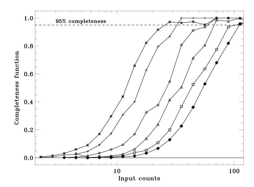
Figure 5.— Completeness functions for different exposure times. From left to right, the functions refer to simulations of 1, 7, 15, 30, 60 and 120 ks exposure time, respectively. The horizontal line shows the 95% completeness.

Figure 6.— 95% completeness threshold in total counts as a function of the exposure time. These values can be modeled by a square root function plus a constant, showing that the algorithm is background limited up to $\gtrsim 100$ ks exposures.

Figure 7.— In the panel ($a$) is shown the distribution of the HRI exposure times and in ($b$) the cumulative distribution. In panel ($c$) is shown the distribution of the galactic column density and in ($d$) the cumulative distribution.

Figure 8.— Measured $\log(N)-\log(S)$ from the analysis of 100 simulated HRI fields (120 ks). The continuous-dashed line marks the input distribution of sources. The derived distribution reproduces the input $\log(N)-\log(S)$ down to a flux of $\sim 3\times 10^{-15}$ erg cm^-2 s^-1. A flux to count rate conversion factor of $1\,{\rm cts\,s^{-1}}=1.71\times 10^{-11}$ erg cm^-2 s^-1 in the 0.5–2.0 keV energy band has been adopted.

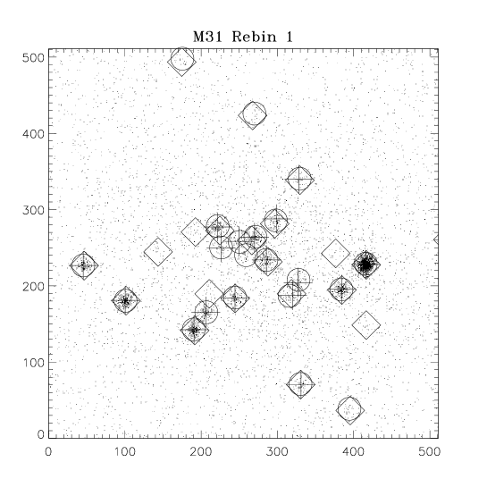
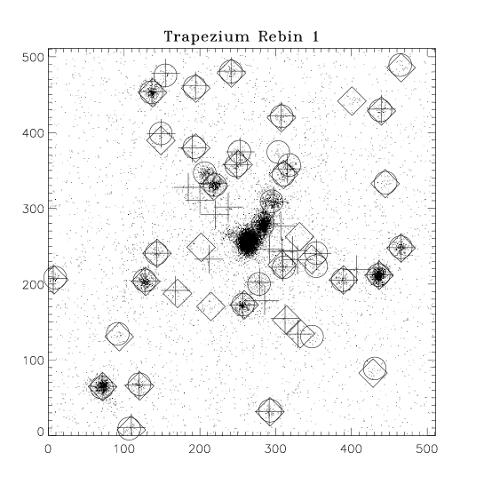
Figure 9.— Source detection in the inner part of the M31 field (left) and of the Trapezium star forming region (right). Sources detected by our WDA are marked by a circle, those by EXSAS with a diamond and those by XIMAGE with a cross.

Figure 10.— See the attached tra_tot.gif file. Source detection in the Trapezium field. The four panels show the (smoothed) images at rebin 1, 3, 6 and 10, respectively. Circles marks X–ray sources. The sizes of the circles is twice the source sigma (modeled as a Gaussian).

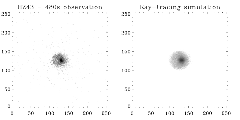
Figure 11.— Comparison between a real $15^{\prime}$ off-axis HRI image of HZ 43 (left panel) with a ray-tracing simulation of a source at the same position.

Table 1Correction factor for the nominal count rate.

Off-axis angle ($\theta$)	Correction ($\alpha$)
$\theta\lesssim 2.1^{\prime}$	$0.18$
$2.1^{\prime}\lesssim\theta\lesssim 6.4^{\prime}$	$0.14$
$6.4^{\prime}\lesssim\theta\lesssim 12.8^{\prime}$	$0.13$
$\theta\gtrsim 12.8^{\prime}$	$-0.02+2.04\times 10^{-2}\times\theta-7\times 10^{-4}\times\theta^{2}$

The nominal count rate $CR$ has to be corrected to account for the non-Gaussianity of the PSF: the corrected count rate is $CR_{c}=(1+\alpha)\,CR$. The off-axis angle $\theta$ in the formula for $\theta\gtrsim 12.8^{\prime}$ (rebin 10) is in arcmin.

Table 2Comparison between the WDA and other source detection algorithms on selected HRI fields.

Field name	Type	ROR	Exposure	BMW	XANADU	MIDAS
		Number	(s)		XIMAGE∗	EXSAS
Trapezium	Star forming region	200500a00	28089	222	249	212
				(38+82+70+32)	(44+64+73+68)	(34+76+73+29)
47 Tuc	Globular cluster	300059a01	13247	10	6	9
				(0+6+2+2)	(0+3+0+3)	(0+6+2+1)
M31	Galaxy	150006n00	30790	85	71	80
				(21+40+18+6)	(17+35+12+7)	(21+35+17+7)
NGC 6633	Open cluster	202056a01	118806	19	5	17
				(1+3+10+5)	(1+2+1+1)	(1+6+8+2)
A 2390	Cluster of galaxies	800346n00	27764	15	23	21
				(3+6+5+1)	(19+2+2+0)	(11+5+5+0)
Kepler§	Supernova Remnant	500099n00	36662	51	129	48
47 Cas§	Bright X–ray star	202057n00	31951	1	24	3

^∗ XIMAGE is not optimised for source detection in ROSAT-HRI images so that a certain number of spurious sources can be found. Moreover, strong sources at off-axis angles larger than $\sim 10^{\prime}$ are often revealed as multiple nearby sources. Source detection has been performed at rebin 1, 3, 6 and 10 separately, masking the relevant inner region.

^§ Images analysed only at rebin 1. 47 Cas has $\sim 20000$ counts (also at 1 spurious source per field, the WDA pick up only one source).

Table 3PSF parameter fits.

Parameter	A	B	C
$\sigma_{1}$	1.87	0.04	0.20
$\sigma_{2}$	3.81	–0.26	0.30
$\sigma_{3}$	31.11	0.44	0.00
$A_{1}\times 10^{2}$	0.28	–0.03	0.00
$A_{2}\times 10^{2}$	7.06	0.79	–0.09
$A_{3}\times 10^{4}$	2.44	0.23	0.02
$\sigma_{g}$	2.59	0.33	0.04
$r_{c}$	24.71	6.75	0.35
$I_{K}$	1.24	0.10	0.02
$A_{g}\times 10^{3}$	9.28	–2.50	2.34
$K_{1}\times 10^{5}$	16.63	0.66	–0.05

Angular dependence of the PSF parameters. Parameters have been fit with a quadratic form $y=A+B\,r+C\,r^{2}$, with $r$ the off-axis radius in arcmin. The normalisations have been chosen such that $\int^{\infty}_{0}PSF(r)\,2\,\pi\,r\,dr=1$. Widths are in arcsec.

References

- (1)
- (2) Angelini, L., Giommi, P.,& White N. E. 1996, in “Röntgenstrahlung from the Universe”, H.U. Zimmermann, J. Trümper, H. Yorke eds., MPE Report, 263, p. 645
- (3)
- (4) Arida, M., et al. (RRA consortium), The ROSAT Results Archive, (e.g. )
- (5)
- (6) Aschenbach, B. 1988, Appl. Opt., 27, 1404
- (7)
- (8) Coupinot, G., Hecquet, J., Aurière, M., & Futually, R. 1992, A&A, 259, 701
- (9)
- (10) Damiani, F., Maggio, A., Micela, G., & Sciortino, S. 1997a, ApJ, 483, 350
- (11)
- (12) Damiani, F., Maggio, A., Micela, G., & Sciortino, S., 1997b, ApJ, 483, 370
- (13)
- (14) David, L. P., et al. 1998, The ROSAT HRI Calibration Report, U.S. ROSAT Science Data Center (SAO)
- (15)
- (16) Fiore, F., Elvis, M., Giommi, P., & Padovani P. 1998, ApJ, 492, 79
- (17)
- (18) Giommi, P., Angelini, L., Jacobs, P., & Tagliaferri, G., 1992, Astronomical Data Analysis Software and Systems I, ASP Conference Series, 1992, D. M. Worrall, C. Biemesderfer and J. Barnes, 25, p. 100
- (19)
- (20) Gotthelf, E.V., & White, N.E., 1997, http://lheawww.gsfc.nasa.gov/users/evg/siscat.html
- (21)
- (22) Grebenev, S. A., Forman, W., Jones, C., & Murray, S., 1995, ApJ, 445, 607
- (23)
- (24) Hasinger, G., et al. 1993, A&A, 275, 1
- (25)
- (26) Hasinger, G., et al. 1998, A&A, 329, 482
- (27)
- (28) Israel, G. L. 1996, Ph.D. Thesis, S.I.S.S.A. Trieste
- (29)
- (30) Lazzati, D., Campana, S., Rosati, P., Tagliaferri, G., & Panzera, M. R. 1999, ApJ in press (Paper I)
- (31)
- (32) Padovani, P., & Giommi P., 1996, MNRAS, 279, 526
- (33)
- (34) Prestwich, A. H., et al. 1998, Spectral calibration of the ROSAT HRI (http://hea-www.harvard.edu/rosat/rsdc_www/HRISPEC/spec_calib.html)
- (35)
- (36) Rosati, P., 1995, Ph.D. Thesis, Università “La Sapienza” di Roma
- (37)
- (38) Rosati, P., Della Ceca, R., Burg, R., Norman, C., & Giacconi R. 1995, ApJ, 445, L11
- (39)
- (40) Slezak, E., de Lapparent, V., & Bijaoui A. 1993, ApJ, 409, 517
- (41)
- (42) Slezak, E., Durret, F., & Gerbal, D. 1994, AJ, 108, 1996
- (43)
- (44) Snowden, S. L. 1994, Cookbook for analysis procedures for ROSAT XRT/PSPC observations of extended objects and diffuse background
- (45)
- (46) Vikhlinin, A., et al., 1995a, ApJ, 451, 542
- (47)
- (48) Vikhlinin, A., et al., 1995b, ApJ, 451, 553
- (49)
- (50) Vikhlinin, A., et al. 1998, ApJ, 502, 558
- (51)
- (52) Voges, W. 1992, in “Proc. ISY Conference”, ESA ISY-3 9
- (53)
- (54) Voges, W. et al., 1996, IAUC, N.6420
- (55)
- (56) White, N. E., Giommi, P., & Angelini, L. 1994, IAUC, N.6100
- (57)
- (58) Zimmermann, H. U. 1994, IAUC, N.6102
- (59)
- (60) Zimmermann, H. U., et al. 1993, Astronomical Data Analysis Software and Systems II, ASP Conference Series, eds. R.J. Hanisch, R.J.V. Brissenden & J. Barnes, Vol. 52, p. 233
- (61)