The Brera Multi-scale Wavelet (BMW) ROSAT HRI source catalog
I: the algorithm

Abstract

We present a new detection algorithm based on the wavelet transform for the analysis of high energy astronomical images. The wavelet transform, due to its multi-scale structure, is suited for the optimal detection of point-like as well as extended sources, regardless of any loss of resolution with the off-axis angle. Sources are detected as significant enhancements in the wavelet space, after the subtraction of the non-flat components of the background. Detection thresholds are computed through Monte Carlo simulations in order to establish the expected number of spurious sources per field. The source characterization is performed through a multi-source fitting in the wavelet space. The procedure is designed to correctly deal with very crowded fields, allowing for the simultaneous characterization of nearby sources. To obtain a fast and reliable estimate of the source parameters and related errors, we apply a novel decimation technique which, taking into account the correlation properties of the wavelet transform, extracts a subset of almost independent coefficients. We test the performance of this algorithm on synthetic fields, analyzing with particular care the characterization of sources in poor background situations, where the assumption of Gaussian statistics does not hold. For these cases, where standard wavelet algorithms generally provide underestimated errors, we infer errors through a procedure which relies on robust basic statistics. Our algorithm is well suited for the analysis of images taken with the new generation of X–ray instruments equipped with CCD technology which will produce images with very low background and/or high source density.

1. Introduction

In the last 20 years the most widely used technique to analyze X–ray images has been the so-called “sliding box” technique: a box of fixed size is passed across an image and sources are identified as enhancements of the total photon counts in the box against the background, which is independently estimated via local or global measurements. This technique has been used in the past to build source catalogs from imaging X-ray missions, such as Einstein (Harris 1990), EXOSAT (Giommi et al. 1991) and ROSAT/PSPC (White, Giommi & Angelini 1994). A different approach has been used in the compilation of the ROSATSRC (Zimmermann 1994) and the Rosat All Sky Survey BSC (Voges et al. 1996) catalogs, where maximum likelihood filters were utilized for source detection and characterization.

Although these catalogs have proven to be extremely useful, they also have shown important limitations. In deep confusion limited images, especially crowded fields, or in the presence of very bright or extended sources (such as clusters of galaxies and supernova remnants), these techniques often tend to blend multiple sources into a single one, to split a bright source in multiple detections and/or to misidentify small background fluctuations as real sources. In addition, these catalogs provide a poor estimate (if any) of the intrinsic source size and the distinction between extended and point-like emission is hardly possible. This means that a visual check “source by source” is required in most cases in order to “clean” the source catalog. An improvement of these techniques has been presented by Vikhlinin et al. 1995, who substituted the sliding box with a matched filter that reproduces at best the profile of point-like sources. This method is optimal for detection of point-like sources, but tends to miss faint sources that are spatially resolved by the detector. The next generation of X–ray missions, with very high sensitivity and spatial resolution, will produce very deep images with a very high surface density of X–ray sources (up to $1000/{\rm deg{{}^{2}}}$) and a level of morphological detail comparable to that of optical images. Therefore, it is important to develop new and more refined techniques for source detection and characterization to fully exploit the scientific content of these vast datasets.

These problems and considerations led to the development of a new generation of detection algorithms in which the square window of the sliding box technique is replaced with a family of filters of different sizes with particular morphological and functional properties: the Wavelet Transform (hereafter WT). The WT is a mathematical tool capable of decomposing an image in a set of sub-images, each representing the image features at a given scale. Sources with sizes ranging from the intrinsic instrumental resolution up to a significant fraction of the whole image can be efficiently extracted at the WT scale that better matches the source size. Moreover WT-based detection algorithms are insensitive to large scale background fluctuations provided that the source size is different from this scale, a typical situation in high energy images.

The application of WT-based algorithms to the automatic detection and characterization of sources in X–ray images was first used by Rosati et al. 1993, 1995 (see also Rosati 1995), who exploited the multi-scale capabilities of this method to compile a catalog of extended sources in ROSAT-PSPC deep pointed observations. This work led to the compilation of the ROSAT Deep Cluster Survey (RDCS; Rosati et al. 1995, 1998), a deep survey of galaxy clusters over $\sim 50$ square degrees. More recently, WT based techniques have been developed and applied by other groups for the analysis of ROSAT, mainly PSPC, images (Grebenev et al. 1995; Harnden et al. 1996; Pislar et al. 1997; Damiani et al. 1997a,b; Vikhlinin et al. 1998), even if a complete catalog of WT detected sources has not been published to date.

In this and in the accompanying paper (Campana et al. 1999; Paper II hereafter) we present a multi-scale wavelet-based algorithm which generalises and combines those used by Rosati et al. 1995 and Lazzati et al. 1998, and its application to the complete archival data of the ROSAT High Resolution Imager (HRI). The paper is organized as follows: in Sect. 2 and 3 we describe how the detection and characterization algorithm works, while in Sect. 4 we test its performances with simulations. Finally, in Sect. 5 we summarize our results and briefly discuss the applications of our algorithm.

2. The detection algorithm

The basic steps of the detection algorithm we developed are summarized in Figure 1, while a more detailed description of single steps is given in the following sections.

First, a wavelet convolution is performed on the X–ray image and an average background value is estimated with a $\sigma$-clipping algorithm (see Sect. 4.1). Given the measured background and referring to the simulations described in Sect. 4, a detection threshold is computed constraining the total average number of spurious detections in the whole image. The source candidates are selected as significant (above the threshold) peaks in each independent wavelet sub-image and a complete catalog is obtained cross-correlating the single-scale catalogs to eliminate multiple-scale detections of the same source and the large-scale blending of nearby small-scale sources.

At this stage, the catalog merely consists of a coarse position and a rough estimate of the count rate and size of the sources. The second part of our algorithm (see lower box of Figure 1) deals with the refinement of these quantities along with their uncertainties and leads to the complete source characterization. To this aim, a model source with a Gaussian point spread function (hereafter PSF) is fitted in wavelet space with a multi-dimensional procedure which takes into account the behavior of the wavelet coefficients both in space and scale. Up to 20 neighbor sources can be fitted simultaneously in the deblending process, thus allowing the characterization of faint objects located near bright sources (see also Lazzati et al. 1998).

As a final result, the algorithm produces - in a fully automated way - a catalog of sources with position, count rate and apparent size along with corresponding uncertainties. For each source the associated probability of spurious detection is also derived.

2.1. The wavelet transform

The wavelet transform of a real function $f$ is the convolution product between $f$ and a class of analyzing wavelets $\psi_{a}(x,y)$, all derived by dilation from a single function $\psi_{1}(x,y)$, called mother wavelet:

$$\psi_{a}(x,\,y)=\frac{1}{a}\psi_{1}(\frac{x}{a},\,\frac{y}{a}).$$ (1)

Any function $g(x,y)$ can be used as the mother for a bidimensional wavelet transform if it satisfies the following conditions:

$$\int_{\mathbb{R}^{2}}|g(x,y)|^{2}\,dx\,dy < \infty$$

$$\int_{\mathbb{R}^{2}}g(x,y)\,dx\,dy < \infty$$ (2)

The above properties assure the existence of the transform of any square integrable function (as astronomical images are) and, more importantly, the fact that, whatever the function $f$ and the scale $a$ of the transform, the mean value of the transformed image is null. This provide an objective and automatic background subtraction in detection applications of the WT.

For a detailed and rigorous analytical description of the wavelet operators, we refer the reader to the extensive reviews published in the astronomical literature (e.g. Grebenev et al. 1995; Slezak et al. 1994) or to more general discussions (Mallat & Hwang 1992; Young 1993) and references therein.

In this work we adopt a discrete approximation of the wavelet operator (see, e.g. Grebenev et al. 1995; Vikhlinin et al. 1998; Lazzati et al. 1998), which keeps all the properties described above provided that the integrals are replaced with discrete summations. This allows faster computations and a reduction of the cross talks between adjacent pixels and scales. The continuous approach, which has been adopted by - e.g. - Damiani et al. 1997a,b, allows the calculation of the transform at whatever scale and position. In this scheme, source characterization proceeds through an iterative refinement of the position and scale at which the transform is calculated.

Our WT computation is based on the multi-resolution theory (Farge 1992) and the “à trous” algorithm (Bijaoui & Giudicelli 1992). We use the ‘mother’ developed by Slezak et al. 1995, which can be analytically approximated with the difference of two Gaussians:

$$\psi_{1}(r) = A\,\exp\left[-{\frac{r^{2}}{2\sigma_{A}^{2}}}\right]-B\,\exp\left[-{\frac{r^{2}}{2\sigma_{B}^{2}}}\right]$$ (3)

$$A \simeq 0.597;\;\;\;\;\;\sigma_{A}\simeq 0.687$$

$$B \simeq 0.264;\;\;\;\;\;\sigma_{B}\simeq 1.030$$

where the $(x,y)$ dependence has been turned into radial due to the symmetry of the mother. This symmetry gives us a new property of the WT operator: it is insensitive to first order derivatives of the transformed function, i.e. the transform of a plane is constantly equal to zero. This means that smoothly varying backgrounds will not affect the significance of the detections. The multi-resolution technique provides us with a sampling on scales logarithmically spaced by a factor of two. According to the wavelet theory (see e.g. Young 1993) this provides the best compromise between completeness and correlation (i.e. redundancies in the wavelet coefficients): a finer sampling would cause an oversampling while a coarser sampling would produce a loss of information. We hence have:

$$a_{j}=2^{j};\qquad j\in\mathbb{N}$$

The sampling in the $x$ and $y$ is performed pixel by pixel, at any scale. This produces an heavy oversampling of the transform, especially at the largest scales, but it does not affect the detection. In the second part of the algorithm, when sources are characterized, a decimation process is applied in order to minimize this oversampling (see Sect. 3.1).

2.2. Detection thresholds

Due to the structure of the wavelet operator, the statistics of coefficients in the WT space cannot in general be handled analytically. If, however, the function $f$ is a white Gaussian noise with mean $\bar{d}$ and dispersion $\sigma_{d}$, we have that the individual WT coefficients are Gaussian distributed according to the law:

$$p(WT) = \frac{1}{\sqrt{2\pi\sigma^{2}}}\,\hbox{exp}\Big{(}-\frac{WT^{2}}{2\sigma^{2}}\Big{)}$$ (4)

$$\sigma = \sqrt{\sigma_{d}^{2}\;\int|\psi|^{2}}$$ (5)

Unfortunately, this is not the case for high energy astronomical images that can be approximated by a white Poisson noise of constant mean (the background), on which sources are overlaid. Since our goal is to assess the probability that the WT peaks are random background realizations, we can neglect the statistics of the sources and concentrate on the transform of pure background. It can be shown (see, e.g. Grebenev et al. 1995) that Equation 5 still holds for a Poisson noise, with

$$\sigma=<WT^{2}>-<WT>^{2}=<WT^{2}>;\quad\sigma_{d}=\sqrt{\bar{d}}$$

however, the probability distribution given by Equation 4 is not followed anymore. Moreover, even if we knew exactly the distribution of the single coefficients, the WT non-orthogonality would prevent us from computing the completeness and contamination of the catalog. Thus, to overcome these problems we must rely on Monte Carlo simulations.

For a set of mean background values between $10^{-4}$ and $10$ counts per pixel we simulated 5000 realizations of random fields, $512\times 512$ pixels each. Then we computed the WT and its standard deviation with Equation 5 and counted all local maxima that exceeded a given signal-to-noise threshold (i.e. the ratio of the wavelet transform and the error given in Equation 5). Since no source has been simulated, any peak in the transformed image is spurious. Repeating this procedure with different thresholds for each scale $a$ of the transform, we have built the integrated probability function of finding a random WT peak exceeding a given signal-to-noise. Figure 2 shows the typical output of a set of simulations with a background of 0.3 counts per pixel. The number of WT peaks that exceeds a given signal-to-noise in the whole field is plotted versus the signal to noise itself for the different scales. To limit the number of spurious detections to, e.g., one in ten fields, we draw a horizontal line corresponding to 0.1 sources and, scale by scale, we set the threshold at the signal to noise where the horizontal line crosses the corresponding curve.

Combining the results of all simulations we obtain the integrated probability function $P$ which, given the number of pixels of the search, the desired signal to noise threshold and the mean value of the background counts, returns the mean expected number of spurious detections. In the algorithm, this function must be inverted. In fact, when we run the WT algorithm on an image, we fix the expected contamination (the number of spurious detections in the whole image) and we compute - as a function of the scale $a$ - the threshold to be used. Note that, since the number of independent points is proportional to the square of the inverse of the scale, the threshold applied on smaller scales will be higher than that on larger scales (see Figure 2).

In principle, the whole set of scales provided by the wavelet transform can be used in the detection procedure. However, in the analysis of high energy images - as those of the ROSAT HRI (see Paper II) - we have a lower scale for the sources set by the instrumental resolution. The analysis on very large scales, say half the size of the image, is strongly contaminated by edge effects and sensitive to residuals from the image reduction. As a general rule, the best scales on which the analysis can be performed are the ones which closely match the instrumental PSF. For these reasons, in the following of this paper and in the analysis of HRI images (Paper II), we will use only the following scales:

$$a=5;\,10;\,20;\,40\quad\hbox{pixels}$$ (6)

where the scale $a$ roughly measures the FWHM of the positive central part of the wavelet filter in pixels.

2.3. Different scales cross-identification

Since the source detection is performed on several scales and given the non-orthogonality of the wavelet operator, a cross-correlation of the single-scale catalogs must be performed. This allows us to get rid of multiple identifications of the same source at different scales and, more importantly, to discriminate true extended sources from a blending of nearby point-like sources. This latter distinction is not trivial, since true extended sources often produce apparently significant peaks in the lower scales, while nearby sources are inevitably blended at larger scales.

First, we eliminate from the catalog multiple scale detection of bright sources on the basis of position and signal-to-noise: among all sources with compatible positions only the most significant (i.e. with the highest signal-to-noise ratio) is held. Two sources detected at different wavelet scales but with nearby positions are matched in a single source if their distance is lower than the scale at which the most significant has been detected.

A more difficult problem is dealing with the merging of nearby sources at large scales. Two or more nearby point-like sources are usually detected as a single extended source at large scales. However, it is also possible that a real extended feature is overlaid on them (a typical situation in supernova remnants and in nearby clusters of galaxies). Our cross-correlation scheme held the large scale detection as a true source only if its significance (signal-to-noise) is larger than that of all lower-scale sources overlaid on it. This scheme slightly favors point-like sources.

The worse situation is provided by a group of weak and close sources, which are detected only at large scales as a single extended feature. This is an intrinsic limitation of the detector resolution that cannot be solved by a detection algorithm, however refined (see, e.g. Damiani et al. 1997a).

Rosati et al. 1995 describe a different scheme, in which all sources are detected and characterized for each scale separately. A subsequent step consists in the cross-correlation of different scale catalogs to get rid of multiple and false detections by means of positional coincidence and fitted count-rates. Damiani et al. 1997a cross-identify only sources detected at consecutive scales and match sources if their distance is less than the scale size corresponding to the maximum signal-to-noise (or 1.5 times the detector PSF).

Albeit simple, our scheme has been shown to be powerful and robust in the analysis of ROSAT HRI fields, that can be very crowded of point sources (see Paper II, in particular Figure 10).

3. Source characterization

After the whole procedure described in last section, we are left with a list of sources with a rough determination of position (the center of the pixel with higher WT coefficient), source size (the scale of the WT where the signal to noise is maximized) and total number of photons (the value of the maximum WT coefficient). Several schemes have been proposed in the literature to refine these estimates in wavelet space; these can be divided in two main groups: fitting the multi-scale profile (e.g. Grebenev et al. 1995; Rosati et al. 1995) or searching for the best position and scale of the source recomputing the WT in a narrower grid both in space and in scale (Damiani et al. 1997a,b).

Our approach is to fit source profiles both in space (as in Rosati et al. 1995) and in scale (as in Grebenev et al. 1995). This allows us to refine simultaneously the position, size and flux of the sources without the need of weight summing parameters derived at different scales. The narrower grid method should in principle be more robust, since it does not involve multi-parameter fitting procedures that could fail when run automatically. However, such a method needs analytic WT computations (instead of our numeric method) and makes it difficult to deal with the strong cross terms in WT space in presence of nearby sources and, more generally, in crowded fields.

3.1. Decimation technique

To apply standard routines ($\chi^{2}$ minimization) to the source characterization in wavelet space, we must first assure that the hypothesis of independence between input data is appropriate. As stated above, this is not the case, mostly at larger scales. Although Rosati 1995 has shown that neglecting the correlations between adjacent data does not significantly compromise the result of the fit, the uncertainties on extracted parameters are highly underestimated and the oversampling in $x,y,a$ lengthens considerably the computing time.

To obtain a fast, robust and unbiased estimate of the source parameters and related errors, we have developed a decimation technique that, taking into account the correlation properties of the WT, extracts a subset of quasi-independent coefficients from the whole transform (see also Lazzati et al. 1998).

Before applying the decimation, we first select a subregion of the transform around the source position. For each detected source, named $\tilde{a}$ the most relevant scale of the detection, a region of radius $4\,\tilde{a}$ centered on the source position is extracted from the whole transform and the scale range is reduced to the set $\{\tilde{a}/2,\,\tilde{a},\,2\,\tilde{a}\}$. Scales smaller than $\tilde{a}/2$ are dominated by noise, while those larger than $2\,\tilde{a}$ suffer from the contamination from adjacent sources. To extract a subset of wavelet coefficients which is almost independent, the minimum distance between two coefficients at a given scale must be almost equal to the correlation length of the transform at this scale, which is proportional to the scale itself. From the analysis of the autocorrelation function of the transform of a pure white noise, we find that the correlation length is given by: $c_{l}(a)\sim 1.7\,a$ (see also Lazzati 1996). At the scales mentioned above we should have, in principle, 69, 17 and 4 orthogonal wavelet coefficients, respectively. Since the most significant coefficient at all scales is the coefficient centered on the source position, we keep it in the decimated set. We finally obtain 61, 17 and 5 coefficients for the three scales. The position of this coefficients for the case $\tilde{a}=5$ is plotted in Figure 3. These extracted coefficients provide us with a small set of almost orthogonal and Gaussian distributed points.

3.2. Source fitting

The model we fit to the decimated set of WT coefficients is the transform of a bidimensional Gaussian. This transform can be computed analytically and can be written as:

$$\tilde{f}(x,y) = 2\pi I_{0}\bigg{[}A\sigma_{A}^{2}\,G\Big{(}x,y,x^{\prime},y^{\prime},\sqrt{\sigma^{2}+2^{2j}\sigma_{A}^{2}}\Big{)}-$$ (7)

$$- B\sigma_{B}^{2}\,G\Big{(}x,y,x^{\prime},y^{\prime},\sqrt{\sigma^{2}+2^{2j}\sigma_{B}^{2}}\Big{)}\bigg{]}$$

where $I_{0}$ is the integral of the source, $\sigma$ its width, $A$, $B$, $\sigma_{A}$ and $\sigma_{B}$ are given in Equation 3 and $G$ is defined as:

$$G(x,y,x^{\prime},y^{\prime},\sigma)=\frac{1}{2\pi\sigma^{2}}\exp\bigg{[}-\frac{(x-x^{\prime})^{2}+(y-y^{\prime})^{2}}{2\sigma^{2}}\bigg{]}$$ (8)

The output of the procedure is hence a set of values $\{x^{\prime},y^{\prime},I_{0},\sigma\}$ along with their errors.

Since our fitting procedure involves scales larger than the natural source scale, it is possible that the WT coefficients are affected by the presence of nearby sources. To deal with this problem, multiple source fitting (up to 20 simultaneous sources) can be performed. Thanks to the linearity of the WT operator, the transform of $N$ sources in a small area is:

$$\tilde{f}(x,y)=\sum_{i=1}^{N}\tilde{f}_{i}(x,y)$$

where $\tilde{f}_{i}(x,y)$ is given by Equation 7. In practice, since it would be meaningless to fit $20\times 4=80$ parameters with only 83 (i.e. $5+17+61$) data and since weak sources could hardly affect the fit of a strong source, the procedure is structured as follows. For each source, the algorithm searches for all sources within ten times its estimated width. In this set of sources, the parameters of those already fitted are freezed while the total counts and sizes of all the other sources are free in the fitting routine. When all sources have been fitted once, the procedure is repeated (improved fit in Figure 1), but this time all nearby sources are held fixed. This multi-source fitting allows a more precise determination of the source fluxes. This is particularly true in the case of very nearby sources where the influence of the negative wings of one source modifies the value of the other source transform (see e.g. Lazzati et al. 1998).

3.2.1 Error determination

If the number of background and source counts is sufficient ($\gtrsim 5\times 10^{-2}$ counts per pixel), a reliable estimate of the parameter uncertainties can be directly obtained from the covariance matrix (see Sect. 4 for more details). However, a more detailed computation of the error on WT coefficients is needed. In fact, Equations 4 and 5 are no longer valid to estimate the WT fluctuations in presence of sources (i.e. non-flat components). A more general form for Equation 5 is given in Grebenev et al. 1995:

$$\sigma(x,y)=\sqrt{f(x,y)\ast|\psi|^{2}}$$ (9)

where $\ast$ represents the convolution product in $\mathbb{R}^{2}$ and $f(x,y)$ is the function to be transformed. Poisson statistics for $f$ has been assumed. Note that Equation 9 is consistent with the results given above when $f=\hbox{const.}$ (cf. Equations 4, 5).

When dealing with very low backgrounds ($\lesssim 5\times 10^{-2}$ counts per pixel), in particular at the lowest scales, the error determination suffers from the strong departure of the WT statistics from the Gaussian case. As a result, errors are generally underestimated. In this case a precise determination in WT space would imply a fitting procedure based on WT statistics which, as stated above, cannot be handled analytically. However, from basic statistics, we can obtain reliable estimates of errors with an a priori method. Let’s consider position $x^{\prime}$ and $y^{\prime}$. If we have a Gaussian shaped spatial distribution of $N$ photons with a width $\Delta$, the precision on the determination of the centroid is limited by:

$$\sigma_{x^{\prime}}\simeq\sigma_{y^{\prime}}\simeq\frac{\Delta}{\sqrt{N-1}}$$ (10)

while the error on total number of counts will be given by Poisson statistics:

$$\sigma_{N}\simeq\sqrt{N}$$ (11)

The intrinsic limit on the width estimate can be expressed through the rms scatter of photon positions:

$$\sigma_{\Delta}\simeq 0.5\,\frac{\Delta}{\sqrt{N-1}}$$ (12)

The final error on fitted parameters is set to be the maximum value between that estimated from the covariance matrix and the above equations.

4. Testing the algorithm

To test the reliability of the source characterization and of the parameter uncertainties, we have simulated a set of $21$ fields with $64$ sources each, for a set of backgrounds ranging from $10^{-3}$ to $10^{-1}$ counts per pixel. Hence, for each background value we have 1344 synthetic sources. The source positions are fixed to an equally spaced $8\times 8$ grid in order to test the accuracy of the fit without edge problems and source confusion (see also Paper II for a complete discussion of this problem). To reproduce at best an astronomical image, the total counts of sources have been simulated according to an Euclidean ${\rm Log}\,N-{\rm Log}\,S$, while all sources have been assumed point-like with a FWHM $\simeq 6$ pixels.

We have then applied the full procedure described above, including background determination and source detection with a threshold of 0.1 spurious sources per simulated field.

4.1. Background determination

The estimate of the mean background value is carried out with a $\sigma$-clipping method. This procedure relies on the hypothesis that the statistics of the image is dominated by two independent distributions: the background counts and the source counts. If the average values of these distributions are strongly different (which is very often the case when dealing with high energy astronomical images) the contribution of sources can be iteratively erased and a robust mean background value measured.

To reach this goal the mean and standard deviation of the whole image are calculated and pixels with a number of counts that exceeds the mean value by more than 3 standard deviations are flagged. The process is repeated iteratively on unflagged pixels until the mean and the standard deviation values converge. Since the $3\,\sigma$-clipping implies Gaussian statistics, the images are binned to obtain an initial mean number of counts per pixel of at least 10.

4.2. Results

These simulations have revealed that as long as the distribution of WT coefficients is well approximated by a Gaussian function, the procedure works very well. With small background values - below $\sim 5\times 10^{-2}$ counts per pixel - the distribution in the lowest scales of WT space becomes increasingly Poissonian and the covariance matrix gives underestimated errors, even if the parameter evaluation remains reliable. In this case, the uncertainties given by Equations 10, 11 and 12 turn out to be more accurate than those obtained in the fitting procedure. Sources with even five input photons (the minimum input value) are detected in the lowest background simulations. This is not a surprising result because, as pointed out by Damiani et al. 1997a, in principle it is possible to detect sources with 3 photons only.

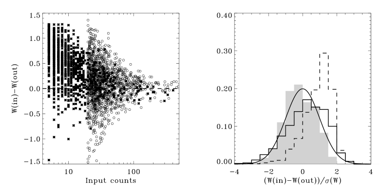
Figures 4, 5 and 6 show the result of these simulations. In all figures, the first panel shows the absolute discrepancy between the input and output parameters (position, total counts and width, respectively) versus the input counts. In the right panels the distribution of the absolute discrepancy between the input and output parameters, divided by the their estimated errors, are compared with a normal Gaussian distribution. Asterisks and dashed lines refer to the lower background ($10^{-3}$ counts per pixel) simulations, while circles and solid lines to a higher background case ($10^{-1}$ counts per pixel).

For low background simulations (dashed lines in Figures 4, 5 and 6) the correlation matrix gives underestimated errors and Equation 10, 11 and 12 are always used. A Kolmogorov-Smirnov (KS) test on the whole set of simulated sources confirms the visual impression that dashed histograms are not incompatible with the Gaussian solid line in the figures. For high background simulations (solid histograms) the correlation matrix is commonly used. Considering the whole set of simulated sources, errors are slightly underestimated (20%, especially in Figure 4). However, a closer inspection reveals that when only bright ($>50$ cts) sources are selected, the estimated errors are Gaussian distributed. We note that the overestimation of fluxes near the detection threshold is common, due to the fact that sources on top of positive background fluctuations are preferentially selected.

Figure 4 shows that source positions are determined with an accuracy which is of the order of the source half width in the low signal-to-noise regime. A similar result is obtained for the total counts (Figure 5). Only for one source out of $2500$ the total counts evaluation has failed by more than a factor of two. This faint source, whose flux and size measurements are affected by a large error, lays in the close vicinity of one of the four significant positive background fluctuations expected (40 simulated fields with 0.1 spurious sources each). The algorithm merged the true source and the fluctuation in a higher flux extended feature. For what concerns the measurement of the source size, Figure 6 shows that particularly in the lower background simulations the width of the source is underestimated. This is due to the fact that, since the vast majority of sources in our simulations are at the limit of detection, those that randomly happen to be more compact have a higher signal-to-noise ratio and are hence preferentially selected by the algorithm against those with lower surface brightness. This bias is present only for weak sources in very low background images and would cause the misidentification of extended sources as point-like and not vice-versa. The shaded region in the right panel of Figure 6 shows how this bias is considerably reduced when only sources with more than 100 counts are considered.

5. Conclusions

We have presented a new detection algorithm based on the wavelet transform for a multi-scale analysis of astronomical X–ray images which is suited for the detection and the characterization of both point-like and extended sources. Given an image in the X-ray band, the algorithm produces a catalog of sources characterized by position, count rate and size along with associated errors.

The main difference of our technique with respect to other WT-based algorithms lies in the source characterization. Our algorithm uses, for the first time, a fitting procedure that models the source in WT-space by taking into account the spatial and multi-scale behavior simultaneously. Moreover, this procedure is performed on a decimated set of wavelet coefficients to drastically reduce the cross-talk between adjacent pixels and scales.

Future high energy missions equipped with CCD detectors, such as XMM, AXAF and JET-X, will combine a high effective area with a small instrumental background. In these cases, current wavelet implementations which rely on Gaussian statistics for the source characterization may not lead to optimal results. The problem of crowded fields has been dealt with a multi-source characterization procedure, where up to 20 sources are fitted simultaneously. In very low background images, this fitting procedure produces reliable parameter estimates but underestimated errors. In these cases we have developed a different error evaluation procedure which relies on basic statistics and which proves to be robust even with vanishing backgrounds.

The use of wavelet-based detection algorithms for the data analysis of the new generation of X–ray missions will provide an accurate, fast and user friendly source detection software. A first application of this algorithm to high resolution X-ray images obtained with the ROSAT HRI is presented in the accompanying paper (Campana et al. 1999) and the analysis of the full set of archival HRI pointings is underway for the construction of a complete wavelet-based catalog of ROSAT HRI X-ray sources.

Figure 1.— Block diagram of the detection and characterization algorithm.

Figure 2.— Threshold determination for detection of sources in wavelet space. The plot shows the number of spurious detections with signal to noise larger than a given value versus the signal to noise itself. The six curves refer to six wavelet scales, from 1.25 to 40 pixels, for simulations with a mean background of 0.3 counts per pixel. The step-like behavior of the smallest scale curve is due to the sensitivity of this scale on the discreteness of the background image. For the four scales used in the search, the signal to noise thresholds relative to a contamination of 0.1 sources per field have been marked.

Figure 3.— Decimation pattern for the three selected WT scales: asterisks mark the smallest scale ($a/2$); diamonds the median scale ($a$) and circles the largest scale ($2\,a$). Note that the largest the scale, the most sparse the WT sampling.

Figure 4.— Simulation results on position accuracy. Left panel shows the absolute error in the X-axis position determination in pixels versus the input counts of the simulated source. Asterisks refer to the $10^{-3}$ counts per pixel background simulations while circles to the $10^{-1}$ counts per pixel simulations. Right panel shows the distribution of position offset normalized to their estimated errors. The curve is a normal Gaussian. Dashed and solid lines refer to the lower and higher backgrounds, respectively.

Figure 5.— Simulation results on total counts determination accuracy. Left panel shows the output counts versus the input counts of all simulated sources. Plotting symbols are analogous to those of Figure 4. Right panel shows the distribution of count differences normalized to their estimated errors. The curve is a normal Gaussian. Dashed and solid lines refer to the lower and higher backgrounds, respectively.

Figure 6.— Simulation results on source width accuracy. Left panel shows the absolute error in the width determination versus the input counts of the simulated source. Plotting symbols are analogous to those of Figure 4. Right panel shows the distribution of size determination differences normalized to their estimated errors. The curve is a normal Gaussian. Dashed and solid lines refer to the lower and higher backgrounds, respectively. The shaded region shows the histogram for the lower background when only bright sources ($>100$ counts) are considered.