Ambipolar Diffusion in YSO Jets

Abstract

We address the issue of ambipolar diffusion in Herbig-Haro jets. The current consensus holds that these jets are launched and collimated via MHD forces. Observations have, however, shown that the jets can be mildly to weakly ionized. Beginning with a simple model for cylindrical equilibrium between neutral, plasma and magnetic pressures we calculate the characteristic time-scale for ambipolar diffusion. Our results show that a significant fraction of HH jets will have ambipolar diffusion time-scales equivalent to, or less than the dynamical time-scales. This implies that MHD equilibria established at the base of a HH jet may not be maintained as the jet propagates far from its source. For typical jet parameters one finds that the length scale where ambipolar diffusion should become significant corresponds to the typical size of large (parsec) scale jets. We discuss the significance of these results for the issue of magnetic fields in parsec-scale jets.

1 INTRODUCTION

Narrow hypersonic jets are a ubiquitous phenomena associated with star formation. In spite of the large database of multi-wavelength observations and numerous theoretical studies, a number of fundamental questions remain unanswered about these jets. Paramount among the outstanding issues is the role of magnetic fields in the launching, collimation and propagation of Young Stellar Object (YSO) jets. The current consensus holds that the jets are formed on small scales ( $L<10~{}AU$) via magneto-centrifugal processes associated with accretion disks (Burrows et al (1996), Shu et al. (1994), Ouyed & Pudritz (1997)). At larger scales, where jet propagation rather than collimation is the issue, there is an implicit assumption that the magnetic fields involved in the launching process will remain embedded in the jets as they traverse the inter-cloud medium. Observations of narrowly collimated jets, or chains of bow-shocks, extending out to parsec scale distances (Reipurth et al. (1997)) has strengthened the viewpoint that the jet beams must “carry their own collimators”. This is based on the possibility that without dynamically significant magnetic fields confining the beam, the jets may be disrupted by hydrodynamical instabilities (Stone et al. (1997), Hardee et al. (1997)).

Do the magnetic fields remain embedded in the jets? That is the question we address in this paper. If we accept that jets are created via MHD forces then the only way to lose the imposed fields is via reconnection or through diffusive processes. The helical topology expected for magneto-centrifugally launched jets would not be likely to lead to large scale reconnection throughout the beam (though reconnection may have important effects on the radiative properties of the jets, Gardiner et al. (1999)). Thus, if magnetic fields can be cleared out of a jet this is more likely to occur via diffusive processes. Large format CCD mosaics have recently demonstrated that YSO jets can extend over multi-parsec length scales ($L_{j}\approx 3$ pc). The dynamical age ($t_{dyn}=L_{j}/V_{j}$) for these jets falls in the range $t_{dyn}=10^{4}~{}-~{}10^{5}$ y (Reipurth et al. (1997), Eisöffel & Mundt (1997)). Thus, even if diffusive processes are slow, they will have a relatively long time to affect the propagation of the beams. In plasmas with less than full ionization, ambipolar diffusion is one of the most effective means of driving the rearrangement of flux relative to the plasma. Observations of optical Herbig-Haro (HH) jets have shown them to be moderately ionized, with ionization fractions ranging from $x=.5~{}-~{}.01$ (Hartigan et al. (1996), Baccioti & Eisöffel (1999)), where the ionization fraction is defined as $x=n_{i}/n_{n}$ and $n_{n}$ and $n_{i}$ are the number densities of neutral and ionized particles respectively. The ionization fractions are seen to fall as the plasma propagates away from internal shocks and may, therefore, fall to even lower values in the optically invisible regions of the beam. Given the potentially low ionization fraction and the extreme ratio of jet radius to length, $R_{j}/L_{j}<10^{-3}$, it may be possible for ambipolar diffusion to significantly alter the MHD equilibria established when the jet was launched.

In this paper we wish to address the issue of ambipolar diffusion in YSO jets. Our present goal is simply to establish the characteristic time and length scales for ambipolar diffusion to operate with respect to the fundamental jet parameters. We leave its consequences to later papers. In section 2 we establish the conditions for an MHD equilibrium in a simplified model of a jet in terms of plasma, neutral and magnetic pressures. In section 3 we consider the equation for ion-neutral drift in this context and in section 4 we present an equation for the ambipolar diffusion time-scale in YSO jets. In section 5 we discuss our results in light of observations and other models.

2 Initial Configuration

We begin by considering the simplest model of a magnetized jet. We imagine a cylindrical column of material of radius $R_{j}$. The column is composed of ions, electrons and neutral species and is initially held together internally by a radial balance of pressure ($P_{i},P_{e},P_{n}$) and magnetic ($\vec{J}\times\vec{B})$ forces. We further assume that the column is in force balance with a (possibly magnetized) ambient medium. Thus, initially, the jet does not expand laterally (i.e., in the radial direction). To simplify our calculation we assume that the temperature of all species is the same ($T_{i}=T_{e}=T_{n}$). We further assume that the magnetic field in the jet is purely poloidal, $\vec{B}=B_{z}(r)\hat{e}_{z}$. Figure 1 shows a schematic of our model for the magnetized jet.

2.1 Global Force Balance

Our calculation is similar to derivations of the ambipolar diffusion time-scale in collapsing molecular clouds (a description of those models can be found in Spitzer (1978) and Mouschovias (1991)). Molecular clouds are cold gravitationally bound systems of extremely low ionization ($x\approx 10^{-6}$). This implies that terms involving gas pressure and ion density can be dropped from consideration when calculating the effects of ambipolar diffusion. Gravity does not, however, play a role in maintaining the cross-sectional properties of a YSO jet and pressure forces can not be ignored. In addition, given the range of ionization fractions in these systems the ion inertia should not, a priori, be dropped from calculations. In what follows we derive a simple expression for the ambipolar diffusion time-scale (based on the ion-neutral drift velocity) including the effects of gas and plasma pressure as well as the ion density.

We begin with the three fluid force balance equations for electrons ($e$), ions ($i$) and neutrals ($n$) which can be written as

$$\rho_{e}{d\vec{v}_{e}\over dt} = -\vec{\nabla}P_{e}-n_{e}e\left(\vec{E}+{\vec{v}_{e}\over c}\times\vec{B}\right)+\vec{F}_{ei}+\vec{F}_{en},$$ (1)

$$\rho_{i}{d\vec{v}_{i}\over dt} = -\vec{\nabla}P_{i}+n_{i}Ze\left(\vec{E}+{\vec{v}_{i}\over c}\times\vec{B}\right)+\vec{F}_{ie}+\vec{F}_{in},$$ (2)

$$\rho_{n}{d\vec{v}_{n}\over dt} = -\vec{\nabla}P_{n}+\vec{F}_{ne}+\vec{F}_{ni},$$ (3)

where the term $d/dt$ represents the convective derivative and $F_{12}$ represents the drag force imparted on species 1 by colliding with species 2. Note that $F_{12}=-F_{21}$.

In what follows we will ignore the electron inertia term. This is valid when the time-scales of interest are long compared with the response time of the electrons. Formally this means that the dynamical time $t_{dyn}$ is longer than either the electron cyclotron period $2\pi/\Omega_{ec}$ or the electron plasma period $2\pi/\omega_{ep}$ (Elliott (1993)) as is the case in YSO jets with fields greater than the $\mu G$ level. We will also neglect the electron collisional coupling to the the neutrals, $F_{en}$, given the difference in masses, $M_{e}<<M_{i},M_{n}$ (see footnote #4 Mouschovias (1996), Ciolek private communication 1999).

With these caveats the addition of equations 1 and 2 yields the following expression:

$$\rho_{i}{d\vec{v}_{i}\over dt}=-\vec{\nabla}(P_{i}+P_{e})+(n_{i}Ze-n_{e}e)\vec{E}+\left({n_{i}Ze\vec{v}_{i}-n_{e}e\vec{v}_{e}\over c}\times\vec{B}\right)+\vec{F}_{in}.$$ (4)

Assuming charge neutrality ($n_{i}Z=n_{e}$) yields the following form for the current density,

$$\vec{J}=n_{i}Ze\vec{v}_{i}-n_{e}e\vec{v}_{e}=n_{e}e(\vec{v}_{i}-\vec{v}_{e}),$$ (5)

and the term with the electric field drops out of equation 4. Making use of Ampére’s law, the Lorentz force can be decomposed into two terms,

$${1\over c}(\vec{J}\times\vec{B})=-\vec{\nabla}_{\perp}{B^{2}\over 8\pi}+{B^{2}\over 4\pi R_{c}}\hat{n}$$ (6)

where $\hat{n}$ is a unit vector directed toward the local center of curvature of the field line, $R_{c}$ is the local radius of curvature, and $\vec{\nabla}_{\perp}$ is the gradient normal to field lines.

Our choice of a $\vec{B}=B_{z}(r)\hat{e}_{z}$ implies that the second term in equation 6 is zero. We are left, therefore, with only the first term which can be identified as the gradient of magnetic pressure, $P_{B}=B^{2}/8\pi$.

Finally, if we add the momentum equations for all three species, again ignoring the electron inertia we arrive at the following equation,

$$\rho_{i}{d\vec{v}_{i}\over dt}+\rho_{n}{d\vec{v}_{n}\over dt}=-\vec{\nabla}(P_{i}+P_{e}+P_{n}+P_{B}).$$ (7)

In what follows we need only consider the radial component of the force equation. Thus if,

$${\partial\over\partial r}(P_{i}+P_{e}+P_{n}+P_{B})=0,$$ (8)

and ${v}_{i,r}={v}_{n,r}={v}_{e,r}=0$ (where the $v_{r}$’s refer to radial velocities) at $t=0$ then the entire configuration begins in equilibrium. It is, however, what we shall call a quasi-equilibrium since each species will be accelerated separately by the terms on the RHS of equations 1 - 3. The plasma and the neutrals will attempt to move past each other as each responds to its own forces. It is only the collisional drag $F_{ij}$ between species which holds the initial configuration together. This is exactly the situation which occurs in a molecular cloud where the cloud can be supported for some period of time by its magnetic field. As in the molecular cloud case, the quasi-equilibrium in the jet can not persist indefinitely and the initial configuration will change on a time-scale $t_{ad}=R_{j}/v_{d}$ where $v_{d}$ is the ion-neutral drift velocity $v_{d}=v_{n}-v_{i}$. We seek to calculate this time-scale.

Note that equation 8 implies that the pressure distributions of the ions and neutrals is not independent.

$${\partial\over\partial r}P_{n}=-{\partial\over\partial r}(P_{i}+P_{e}+P_{B})$$ (9)

We will use this relation below in our calculation of $t_{ad}$.

3 The Ion-Neutral Drift

If we divide equation 4 by $\rho_{i}$ and subtract from it equation 3 (itself divided by $\rho_{n}$) we find,

$${d\vec{v}_{i}\over dt}-{d\vec{v}_{n}\over dt}=-{1\over\rho_{i}}\vec{\nabla}(P_{i}+P_{e}+P_{B})+{1\over\rho_{n}}\vec{\nabla}P_{n}+\vec{F}_{in}\left({\rho_{n}+\rho_{i}\over\rho_{n}\rho_{i}}\right).$$ (10)

If we now assume that the collisions will quickly bring the ion-neutral drift to a steady velocity, i.e., the relative accelerations approach zero after a few collisions, we have the following radial balance equation between collisions and hydro-magnetic forces,

$$F_{in}\left({\rho_{n}+\rho_{i}\over\rho_{n}\rho_{i}}\right)={1\over\rho_{i}}{\partial\over\partial r}(P_{i}+P_{e}+P_{B})-{1\over\rho_{n}}{\partial\over\partial r}P_{n}.$$ (11)

Substituting equation 9 into the above expression we find the densities cancel, leading to

$${F}_{in}={\partial\over\partial r}(P_{i}+P_{e}+P_{B}).$$ (12)

We now make the approximation that the scale of the gradients in the jet are such that

$${\partial P_{k}\over\partial r}\approx{P_{k}\over R_{j}}$$ (13)

where $P_{k}$ is is the characteristic scale for that pressure of the k-th component of the configuration. We also use the definition of the plasma $\beta$ parameter, $\beta=P_{g}/P_{B}$, where $P_{g}=P_{i}+P_{e}$. Thus

$$F_{in} = {P_{B}\over R_{j}}(\beta+1)$$ (14)

$$= {{B}^{2}\over 8\pi R_{j}}(\beta+1).$$ (15)

To reduce this equation further we must consider the form of the collisional force. $F_{in}$ can be written as,

$$\vec{F}_{in}=\rho_{i}\rho_{n}{\langle\sigma w\rangle_{in}\over M_{i}+M_{n}}(\vec{v_{n}}-\vec{v_{i}}),$$ (16)

where $\langle\sigma w\rangle_{in}\approx 3\times 10^{-9}~{}cm^{3}~{}s^{-1}$ is the average collision rate (Spitzer (1978)). We can now solve for the ion-neutral drift velocity.

$$v_{d}={M_{i}+M_{n}\over 8\pi}{1\over\langle\sigma w\rangle_{in}}\left({B^{2}\over\rho_{i}\rho_{n}R_{j}}\right)(\beta+1).$$ (17)

Thus the time-scale for changes in the initial configuration can be written as

$$t_{ad}={8\pi\langle\sigma w\rangle_{in}M_{n}M_{i}\over M_{i}+M_{n}}x\left({n_{n}R_{j}\over B}\right)^{2}(\beta+1)^{-1},$$ (18)

where we have used $x=n_{i}/n_{n}$. The above expression gives the ambipolar diffusion time-scale in terms of the fundamental parameters in the jet ($x,n_{n},R_{j}$ and $B$).

4 Ambipolar Diffusion in YSO Jets

Of the four variables in equation 18 only first three ($x$, $n_{n}$, $R_{j}$) are well characterized for HH jets. From observations typical values are: $.01\leq x\leq.1$; $10^{3}\leq n_{n}/~{}cm^{-3}\leq 10^{4}$; $1\times 10^{15}~{}\leq R_{j}/~{}cm\leq 5\times 10^{15}$ (Baccioti & Eisöffel (1999)). Magnetic fields however are not so easily categorized. To date there have been only a handful of measurements of fields in YSO jets (Ray et al. (1997)). Thus, it would be better to cast equation 18 in terms of a parameter such as the temperature which has been measured in many YSO jets. Typical values in optical jets are $5\times 10^{3}~{}K<T<3\times 10^{4}~{}K$, (Baccioti & Eisöffel (1999)). To express equation 18 in terms of T we use our assumption that the electron and ion temperature is the same and, furthermore, assume that the plasma is mainly composed of Hydrogen atoms. Thus

$$M_{i} = M_{n}$$ (19)

$$n_{i} = n_{e}$$ (20)

$$P_{e}=n_{e}kT = n_{i}kT=P_{i}$$ (21)

The magnetic field can now be expressed as

$$B^{2}=8\pi\frac{P_{e}+P_{i}}{\beta}=16\pi n_{i}kT{1\over\beta},$$ (22)

and the ambipolar diffusion time-scale becomes

$$t_{ad}={M_{n}\langle\sigma w\rangle_{in}\over 4k}\left({n_{n}R_{j}^{2}\over T_{j}}\right)\left({\beta\over\beta+1}\right).$$ (23)

Upon normalization the ambipolar diffusion time-scale can be written as

$$t_{ad} = 28,904\left({n_{n}\over 10^{3}cm^{-3}}\right)\left({R_{j}\over 10^{15}cm}\right)^{2}\left({10^{4}K\over T_{j}}\right)Q(\beta)~{}y$$ (24)

$$Q(\beta) = \left({\beta\over\beta+1}\right)$$ (25)

Note that $Q(\beta)$ is positive with an asymptotic value of $1$ as $\beta\rightarrow\infty$.

This shows that the ion-neutral drift can be driven by gas pressure forces alone if the individual species’ pressure gradients have different signs, an artificial situation not likely to be encountered in real jets. Detailed calculations of equilibrium magnetically confined jets arising from accretion disks indicate that $\beta$ can become quite low in some regions of the jet. As an example, we provide in Figure 2 a plot of $\beta$ versus radius for an equilibrium MHD jet. This model was calculated via the Given Inner Geometry method of Lery et al. (Lery et al. (1998), Lery et al. (1999)) for determining the asymptotic structure of magneto-centrifugally launched flows. Figure 2 shows that $\beta$ can drop to values below $\beta=1$ in the inner regions of the jet ($r<R_{j}$).

In Figure 3 and 4 we show surface plots of $t_{ad}~{}vs~{}\beta$ for $\beta=1$ and $\beta=.1$. From equations 25 and 26 and these figures it is clear that depending on the conditions in the jets, $t_{ad}$ can become as large as $10^{6}$ y and as small as $10^{3}$ y. For jet parameters in the middle of the expected range of variation we find $t_{ad}$ of order $10^{5}$ to $10^{4}$ y. What is noteworthy about these results is a significant region of parameter space exists where the dynamical time-scale for YSO jets is of order of, or greater than, the ambipolar diffusion time: $t_{dyn}>t_{ad}$. Thus ambipolar diffusion is likely to play a role in the dynamics of large scale YSO jets and outflows. We discuss the consequences of this conclusion in the next section.

5 Discussion and Conclusions

Our conclusion that ambipolar diffusion time-scales can be comparable to jet dynamical lifetimes raises a number of intriguing issues. The first is the most obvious. Ambipolar diffusion will rearrange the mass to flux ratio in the jet and alter any initial equilibrium between the plasma, neutrals and magnetic field. Our analysis is too simplified to yield conclusions about how the jet will evolve in the presence of ambipolar diffusion. In our analysis we did not consider the effect of toroidal fields. The hoop stresses associated with toroidal fields will the pull ions towards the jet axis. Thus depending on the orientation of the magnetic pressure gradients, magnetic forces (pressure and tension) can either compete or apply forces in the same direction. Including a toroidal component does not, in general, change the order of magnitude of the ambipolar diffusion time-scale, however, it can change the direction in which the ions are pushed. The plasma and magnetic field may bleed out of the jet leaving only the neutrals or, conversely, strong hoop stresses could draw the plasma and field in towards the jet axis. In both cases, however, the neutrals will be free to contract or expand depending on their pressure distribution relative to the ambient medium. Thus one expects a potentially significant rearrangement of the jet’s cross sectional properties when ambipolar and jet time-scales are comparable. The consequences of ambipolar diffusion on long term jet propagation should, therefore, be investigated in detail.

The possibility that many jets will have $t_{dyn}\approx t_{ad}$ is suggestive for the general issue of YSO outflows. There remains considerable debate over the connection between HH jets and molecular outflows (Masson & Chernin (1993), Cabrit (1997)). The discovery of parsec scale “superjets” (Reipurth et al. (1997), Eisöffel & Mundt (1997)) has strengthened the case for jets as the source of molecular outflows by extending jet lifetimes. Still, most outflows have larger dynamical timescales than even the superjets by a factor of at least a few. One may wonder then why the jets have shorter lifetimes then the molecular outflows. Our results suggest that in some systems at least it is ambipolar diffusion which sets the lifetime of the visible collimated jet. Converting to consideration of length scales, if one takes the minimum ambipolar diffusion time from our calculation, $t_{ad}\approx 10^{3}~{}y$ and the minimum characteristic jet velocity, $V_{j}\approx 10^{2}~{}km/s$ one finds the minimum distance where ambipolar diffusion becomes effective: $D_{ad}\approx 0.3~{}pc$ Our results indicate that ambipolar diffusion should not be effective before a jet reaches this distance. Moreover for typical values $t_{ad}\approx 10^{4}~{}y$ and $V_{j}\approx 3\times 10^{2}~{}km/s$ one finds $D_{ad}\approx 3~{}pc$. It is indeed noteworthy that this value corresponds well with the distance where the longest jets start to fade away. When $t_{dyn}$ becomes comparable to $t_{ad}$ the beam may no longer be confined by magnetic forces.

Figure 1: Cartoon of Jet Model. Shown is a section of a magnetized jet composed of a plasma, neutral gas and magnetic field oriented along the axis of the jet. The pressure and field distributions are a function of cylindrical radius only.

Figure 2: Plasma beta vs jet radius for MHD equilibrium jet. Jet model taken from calculations of Lery et al. 1999. Note that lowest values of beta occur within

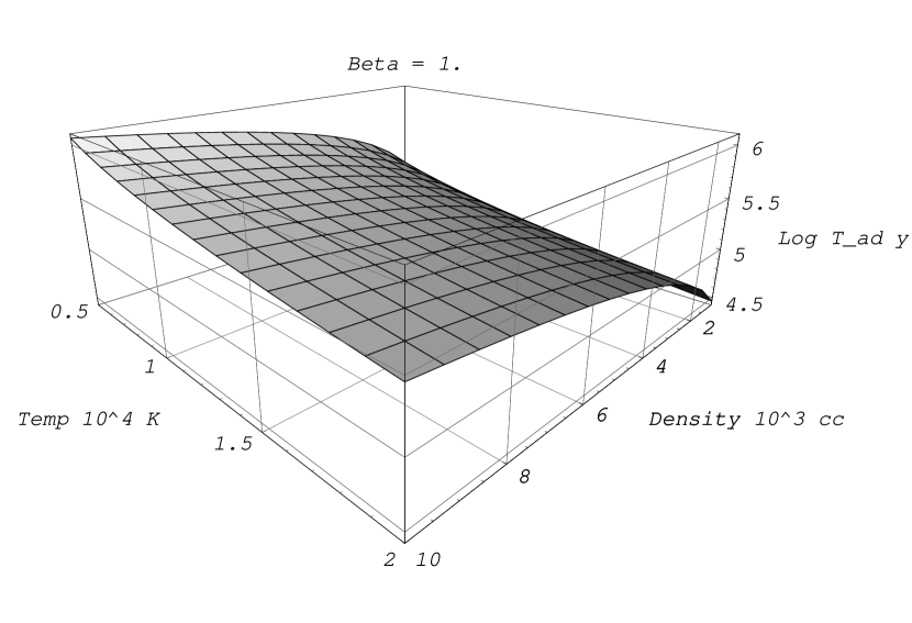
Figure 3: The Ambipolar diffusion time-scale as a function of temperature (in units of 10,000 K) and density (in units of 1000 $cm^{-3}$) when $\beta=1$. The jet radius is $2\times 10^{15}$ cm.

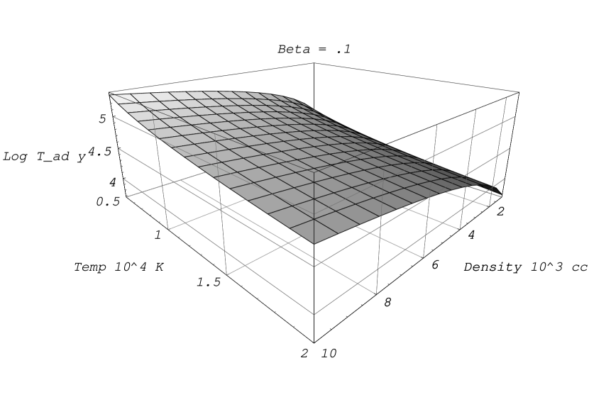
Figure 4: The Ambipolar diffusion time-scale as a function of temperature (in units of 10,000 K) and density (in units of 1000 $cm^{-3}$) when $\beta=.1$. The jet radius is $2\times 10^{15}$ cm.

References

- Blandford & Payne (1982) Blandford, R. D. & Payne, D. G. 1982, MNRAS, 199, 883.
- Blondin et al. (1990) Blondin, J. M., Fryxell, B. A. & Königl, A. 1990, ApJ, 360, 370.
- Burrows et al (1996) Burrows, C., Stapelfeldt, K., Watson, A., Krist, J.E., Ballester, K., Clarke, J., Crisp, D., Gallagher, J., Griffiths, R., Hester, J., Hoessel, J., Holtzman, J., Mould, J., Scowen, P., Trauger, J., & Westphal, J., 1996, ApJ, 473, 437
- Baccioti & Eisöffel (1999) Baccioti, F. & Eisoffel, J., 1999, A&A, in press
- Cabrit (1997) Cabrit, S., 1997, in Herbig-Haro Flows and the Birth of Low Mass Stars, in IAU Symposium no. 182, eds B. Reipurth & C Bertout, (Kluwer, Dordrecht)
- Cerqueira et al. (1998) Cerqueira, A. H., Gouveia Dal Pino, E. M., & Herant, M. 1998, ApJ, 489, L185.
- Cerqueira et al. (1999) Cerqueira, A. H., Gouveia Dal Pino, E. M., & Herant, M. 1998, ApJ, in press
- Clarke et al. (1986) Clarke, D., Norman, M., & Burns, J., 1986, ApJ, 311L, 63
- Eisöffel & Mundt (1997) Eisloffel, J & Mundt, R. 1997, AJ, 114, 280
- Elliott (1993) Elliott, J. A., 1993, in Plasma Physics, An Introductory Course, ed R. Dendy, (Cambridge University Press, Cambridge)
- Frank et al. (1998) Frank, A., Ryu, D., Jones, T. W. & Noriega-Crespo, A. 1998, ApJ, 494, L79.
- Frank et al. (1999) Frank, A., Lery, T., Gardiner, T., Ryu, D., & Jones, T. W., 1999, ApJ, submitted
- Gardiner et al. (1999) Gardiner, T., Frank, A., Ryu, D., Jones, T., 1999, ApJ, submitted
- Hartigan et al. (1996) Hartigan, P, Morse, J, Raymond, J, 1995, ApJ, 444, 943
- Hardee et al. (1997) Hardee, P., Clarke, D., & Rosen, A., 1997, ApJ, 485, 533
- Lery et al. (1998) Lery T., Heyvaerts J., Appl S., Norman C.A., 1998, A&A, 337, 603
- Lery et al. (1999) Lery T., Heyvaerts J., Appl S., Norman C.A., 1999, A&A, accepted
- Lind et al. (1989) Lind, K., Payne, D., Meier, D., & Blandford, R., 1989,ApJ, 344,.89
- Mouschovias (1991) Mouschovias, T. 1991, in “The Physics of Star Formation and Early Stellar Evolution”, eds. C.J. Lada and N.D. Kylafis, NATO ASI Series (Kluwer)
- Mouschovias (1996) Mouschovias, T. 1996, in “Solar and Astrophysical Magnetohydrodynamic Flows” , eds. K. Tsinganos (Dordrecht, Kluwer)
- Masson & Chernin (1993) Masson, C, Chernin, L., 1993, ApJ, 414, 230
- Mouschovias & Paleologou (1981) Mouschovias, T., Paleologou, E., 1981, ApJ, 246, 64
- Ouyed & Pudritz (1997) Ouyed, R. & Pudritz, R. E. 1997a, ApJ, 482, 712.
- (24) Ouyed, R. & Pudritz, R. E. 1997b, ApJ, 484, 794.
- Ray et al. (1997) Ray, T. P., Muxlow, T. W. B., Axon, D. J., Brown, A., Corcoran, D., Dyson, J. & Mundt, R. 1997, Nature, 385, 415.
- Reipurth et al. (1997) Reipurth, B., Bally, J. & Devine, D. 1997, ApJ, 114, 2708.
- Romanova et al. (1998) Romanova, M. M., Ustyugova, G. V., Koldoba, A. V., Chechetkin, V. M., & Lovelace, R. V. E. 1998, ApJ, 500, 703.
- Shu et al. (1994) Shu, F., Najita, J., Ostriker, E., Wilkin, F., Ruden, S., & Lizano, S., 1994, ApJ 429, 781
- Spitzer (1978) Spitzer, L., 1978, Physical Processes in the Interstellar Medium, (John Wiley, New York)
- Stone et al. (1997) Stone, J, Xu, J., & Hardee,P., 1997, ApJ, 483, 136
- Todo et al. (1992) Todo, Y., Uchida, Y., Sato, T., & Rosner, R.,1992, PASJ, 44,245
- Zinnecker et al. (1998) Zinnecker, H., McCaughrean, M. J. & Rayner, J. T. 1998, Nature, 394, 862.