Test of high–energy interaction models using the hadronic core of EAS

Abstract

Using the large hadron calorimeter of the KASCADE experiment, hadronic cores of extensive air showers have been studied. The hadron lateral and energy distributions have been investigated in order to study the reliability of the shower simulation program CORSIKA with respect to particle transport, decays, treatment of low–energy particles, etc. A good description of the data has been found at large distances from the shower core for several interaction models. The inner part of the hadron distribution, on the other hand, reveals pronounced differences among interaction models. Several hadronic observables are compared with CORSIKA simulations using the QGSJET, VENUS and SIBYLL models. QGSJET reproduces the hadronic distributions best. At the highest energy, in the 10 PeV region, however, none of these models can describe the experimental data satisfactorily. The expected number of hadrons in a shower is too large compared to the observed number, when the data are classified according to the muonic shower size.

[Test of high energy interaction models]

• Institut für Kernphysik and Institut für Experimentelle Kernphysik, Forschungszentrum and Universität Karlsruhe, P.O. Box 3640, D–76021 Karlsruhe, Germany

• Institute for Nuclear Studies and Dept. of Experimental Physics, University of Lodz, PL–90950 Lodz, Poland

• Institute of Physics and Nuclear Engineering, RO–7690 Bucharest, Romania

• Cosmic Ray Division, Yerevan Physics Institute, Yerevan 36, Armenia

1 Proem

The interpretation of extensive air shower (EAS) measurements in the PeV domain and above relies strongly on the hadronic interaction model applied when simulating the shower development in the Earth’s atmosphere. Such models are needed to describe the interaction processes of the primary particles with the air nuclei and the production of secondary particles.

In the EAS Monte Carlo codes the electromagnetic and weak interactions can be calculated with good accuracy. Hadronic interactions, on the other hand, are still uncertain to a large extent. A wealth of data exists on particle production from $p\overline{p}$ colliders up to energies which correspond to 2 PeV/c laboratory momentum and from heavy ion experiments up to energies of 200 GeV/nucleon. However, almost all collider experiments do not register particles emitted in the very forward direction where most of the energy flows. These particles carry the preponderant part of the energy and, therefore, are of utmost importance for the shower development of an EAS. Since most of these particles are produced in interactions with small momentum transfer, QCD is at present not capable of calculating their kinematic parameters.

Many phenomenological models have been developed to reproduce the experimental results. Extrapolations to higher energies, to small angles, and to nucleus–nucleus collisions have been performed under different theoretical assumptions. The number of participant nucleons in the latter case is another important parameter which influences the longitudinal development of a shower. Many EAS experiments have used specific models to determine the primary energy and to extract information about the primary mass composition. Experience shows that different models can lead to different results when applied to the same data.

Therefore, it is of crucial importance to verify the individual models experimentally as thoroughly as possible. When planning the KASCADE experiment, one of the principal motivations to build the hadron calorimeter was the intention to verify available interaction models by studying the hadronic central core. In the Monte Carlo code CORSIKA [1] five different interaction codes have been implemented and placed at the users’ disposal. By examining the hadron distribution in the very centre these interaction models are tested. The propagation code itself, viz. hadron transport, decay modes, scattering etc., is checked by looking to the hadron lateral distribution further outside up to distances of 100 m from the core.

2 The apparatus

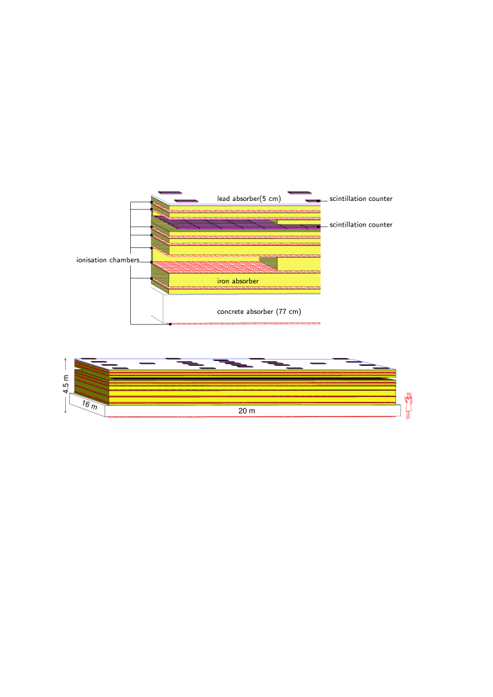
Figure 1: Sketch of the KASCADE central calorimeter. Detailed view (top) and total view (bottom).

The KASCADE experiment consists of an array of 252 stations for electron and muon detection and a calorimeter in its centre for hadron detection and spectroscopy. It has been described in detail elsewhere [2]. The muon detectors in the array are positioned directly below the scintillators of the electron detectors and are shielded by slabs of lead and iron corresponding to 20 radiation lengths in total. The absorber imposes an energy threshold of about 300 MeV for muon detection.

The calorimeter is of the sampling type, the energy being absorbed in an iron stack and sampled in eight layers by ionisation chambers. Its performance is described in detail by Engler et al. [3]. A sketch of the set–up is shown in Fig. 1. The iron slabs are 12–36 cm thick, becoming thicker in deeper parts of the calorimeter. Therefore, the energy resolution does not scale as $1/\sqrt{E}$, but is rather constant varying slowly from $\sigma/E=20\%$ at 100 GeV to 10% at 10 TeV. The concrete ceiling of the detector building is the last part of the absorber and the ionisation chamber layer below acts as tail catcher. In total, the calorimeter thickness corresponds to 11 interaction lengths $\lambda_{I}$ for vertical hadrons. On top, a 5 cm lead layer filters off the electromagnetic component to a sufficiently low level.

The liquid ionisation chambers use the room temperature liquids tetramethylsilane (TMS) and tetramethylpentane (TMP). A detailed description of their performance can be found elsewhere [4]. Liquid ionisation chambers exhibit a linear signal behaviour with a very large dynamic range. The latter is limited only by the electronics to about $5\times 10^{4}$ of the amplifier rms–noise, i.e., the signal of one to more than $10^{4}$ passing muons, equivalent to 10 GeV deposited energy, is read out without saturation. This ensures the energy of individual hadrons to be measured linearly up to 20 TeV. At this energy, containment losses are at a level of two percent. They rise and at 50 TeV signal losses of about 5% have to be taken into account. The energy calibration is performed by means of through–going muons taking their energy deposition as standard. Electronic calibration is repeated in regular intervals of 6 months by injecting a calibration charge at the amplifier input. A stability of better than 2% over two years of operation has been attained. The detector signal is shaped to a slow signal with $10~{}\mu$s risetime in order to reduce the amplifier noise to a level less than that of a passing muon. On the other hand, this makes a fast external trigger necessary.

The principal trigger of KASCADE is formed by a coincident signal in at least five stations in one subgroup of 16 stations of the array. This sets the energy threshold to a few times $10^{14}$ eV depending on zenith angle and primary mass. An alternative trigger is generated by a layer of plastic scintillators positioned below the third iron layer at a depth of $2.2~{}\lambda_{I}$. These scintillators cover two thirds of the calorimeter surface and deliver timing information with 1.5 ns resolution.

3 Simulations

EAS simulations are performed using the CORSIKA versions 5.2 and 5.62 as described in [1]. The interaction models chosen in the tests are VENUS version 4.12 [5], QGSJET [6] and SIBYLL version 1.6 [7]. We have chosen two models which are based on the Gribov Regge theory because their solid theoretical ground allows best to extrapolate from collider measurements to higher energies, forward kinematical regions, and nucleus–nucleus interactions. The DPMJET model, at the time of investigations, was not available in CORSIKA in a stable version. In addition, SIBYLL was used, a minijet model that is widely used in EAS calculations, especially as the hadronic interaction model in the MOCCA code. A sample of 2000 proton and iron–induced showers were simulated with SIBYLL and 7000 p and Fe events with QGSJET. With VENUS 2000 showers were generated, each for p, He, O, Si and Fe primaries. The showers were distributed in the energy range of 0.1  PeV up to 31.6  PeV according to a power law with a differential index of -2.7 and were equally spread in the interval of $15^{o}$ to $20^{o}$ zenith angle. In addition, the changing of the index to -3.1 at the knee position, which is assumed to be at 5 PeV, was taken into account. The shower axes were spread uniformly over the calorimeter surface extended by 2 m beyond its boundary.

In order to determine the signals in the individual detectors, all secondary particles at ground level are passed through a detector simulation program using the GEANT package [8]. By these means, the instrumental response is taken into account and the simulated events are analysed in the same way as the experimental data, an important aspect to avoid systematic biases by pattern recognition and reconstruction algorithms.

4 Shower size determination

The data evaluation proceeds via three levels. In a first step the shower core and its direction of incidence are reconstructed and, using the single muon calibration of the array detectors, their energy deposits are converted into numbers of particles. In the next stage, iterative corrections for electromagnetic punch–through in the muon detectors and muonic energy deposits in the electron detectors are applied. The particle densities are fitted with a likelihood function to the Nishimura Kamata Greisen (NKG) formula [9]. A radius parameter of 89 m and 420 m is used for electrons and muons, respectively. Because of limited statistics, the radial slope parameter (age) is fixed for the muons. The radius parameters deviate from the parameters originally proposed, but have been found to yield the best agreement with the data. The muon fit extends from 40 m to 200 m, the lower cut being imposed by the strong hadronic and electromagnetic punch–through near the shower centre. The upper boundary reflects the geometrical acceptance. In a final step, the muon fit function is used to correct the electron numbers and vice versa.

The electromagnetic and muonic sizes $N_{e}$ and $N_{\mu}$ are obtained by integrating the final NKG fit functions. For the muons alternatively, integration within the range of the fit results in a truncated muon number $N^{\prime}_{\mu}$. This observable has the advantage of being free of systematical errors caused by the extrapolation outside the experimental acceptance. As demonstrated in Fig. 2, it yields a good estimate of the primary energy irrespective of primary mass. To a certain extent, it is an integral variable indicating the sum of particles produced in the atmosphere independently of longitudinal cascade development. In the lefthand graph, the simulated values for the QGSJET model are plotted together with fitted straight lines. They show that in the $N^{\prime}_{\mu}$ range given, the primary energy is proportional to the muon number $E_{0}\propto N_{\mu}^{\prime 0.98}$ with an error in the exponent of 0.06. This holds for the selected showers hitting the central detector with their axes. (For all showers falling into the area of the array a slightly higher coefficient of 1.10 is found.)

It has been checked that the particle numbers are evaluated correctly up to values of $\lg N^{\prime}_{\mu}=5$. At the highest energy of 100 PeV simulations indicate that $N^{\prime}_{\mu}$ is overestimated by about 10%. By studying $N_{\mu}$ sizes at this energy experimentally, irregularities in the muon size distribution may indicate an overestimation of 20%. How well different models agree among each other is shown on the righthand part of Fig. 2, where the corresponding fitted lines are presented. It is seen that the SIBYLL model lies above the two others. In other words it generates fewer muons with consequences that will be discussed below. It is this truncated muon number $N^{\prime}_{\mu}$ which we shall use throughout this article to classify events according to the muon number, that means approximately according to the primary energy.

The accuracy of the reconstructed shower sizes is estimated to be 5% for $N_{e}$ and 10% for $N^{\prime}_{\mu}$ around the knee position.

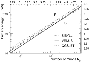
Figure 2: Primary energy as determined by simulations from the truncated muon number $N^{\prime}_{\mu}$ using the interaction models indicated. The vertical bars indicate the rms widths of primary energy distribution for fixed number of muons.

5 Hadron reconstruction

The raw data of the central detector are passed through a pattern recognition program which traces a particle in the detector and reconstructs its position, energy and incident angle. Two algorithms exist. One of them is optimized to reconstruct unaccompanied hadrons and to determine their energy and angle with best resolution. The second is trained to resolve as many hadrons as possible in a shower core and to reconstruct their proper energies and angles of incidence. This algorithm has been used for the analyses presented in the following. Grosso modo, the pattern recognition proceeds as follows: Clusters of energy are searched to line up and to form a track, from which roughly an angle of incidence can be inferred. Then in the lower layers patterns of cascades are looked for since these penetrating and late developing cascades can be reconstructed most easily. Going upwards in the calorimeter, clusters are formed from the remaining energy and lined up to showers according to the direction already found. The uppermost layer is not used for hadron energy determination to evade hadron signals, which are too much distorted by the electromagnetic component, nor is the trigger layer used because of its limited dynamical range.

Due to a fine lateral segmentation of 25 cm, the minimal distance to separate two equal–energy hadrons with 50% probability amounts to 40 cm. This causes the reconstructed hadron density to flatten off at about 1.5 hadrons/m². The reconstruction efficiency with respect to the hadron energy is presented in Fig. 4. At 50 GeV an efficiency of 70% is obtained. This energy is taken as threshold in most of the analyses in the following, if not mentioned otherwise. We present the values on a logarithmic scale in order to demonstrate how often high–energy radiating muons can mimic a hadron. Their reconstructed hadronic energy, however, is much lower, typically by a factor of 10. The fraction of non–identified hadrons above 100 GeV typically amounts to 5%. This value holds for a 1 PeV shower hitting the calorimeter at its centre and rises to 30% at 10 PeV. This effect is taken into account automatically, because in the simulation it appears as the same token.

6 Event selection

About $10^{8}$ events were recorded from October 1996 to August 1998. In $6\times 10^{6}$ events, at least one hadron was reconstructed. Events accepted for the present analysis have to fulfill the following requirements: More than two hadrons are reconstructed, the zenith angle of the shower is less than $30^{\circ}$ and the core, as determined by the array stations, hits the calorimeter or lies within 1.5 m distance outside its boundary. For shower sizes corresponding to energies of more than about 1 PeV, the core can also be determined in the first calorimeter layer by the electromagnetic punch–through. The fine sampling of the ionisation chambers yields 0.5 m spatial resolution for the core position. For events with such a precise core position it has to lie within the calorimeter at 1 m distance from its boundary. After all cuts, 40 000 events were left for the final analysis.

For non–centric showers, hadronic observables like the number of hadrons have been corrected for the missing calorimeter surface by requiring rotational symmetry. On the other hand, some variables are used, for which such a correction is not obvious, e.g. the minimum–spanning–tree, see Section 8.4. In these cases, only a square of $8\times 8~{}\mbox{m}^{2}$ of the calorimeter with the shower core in its centre is used and the rest of the calorimeter information neglected. This treatment ensures that all events are analysed on the same footing.

7 Tests at large distances

Figure 3: Reconstruction efficiency for hadrons for two different zenith angles. The square symbols represent the probability of radiating muons misidentified as hadrons.

Figure 4: Density of hadrons (left scale) and of hadronic energy (right scale) for showers of truncated muon numbers as indicated corresponding to primary energies of 3–10 PeV. The curves represent fits of the NKG formula to the data.

Figure 5: Density of hadronic energy (filled circles) vs. core distance for two intervals of primary energy. The indicated muon numbers correspond to $1~{}\mbox{PeV}\leq E_{0}<3~{}\mbox{PeV}$ and $3~{}\mbox{PeV}\leq E_{0}<10~{}\mbox{PeV}$. The CORSIKA simulations (open symbols) represent primary proton and iron nuclei with the QGSJET model.

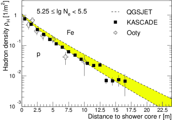
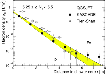
Figure 6: Lateral hadron density for electromagnetic shower sizes of $5.25\leq\lg N_{e}<5.5$. Thresholds for hadron detection are 50 GeV (left), and 1 TeV (right). The dashed lines represent CORSIKA simulations with the QGSJET model for primary proton and iron nuclei using an exponential, see text.

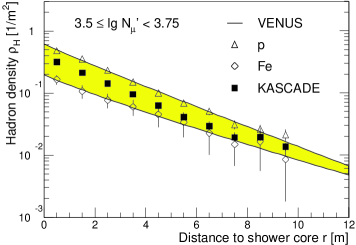
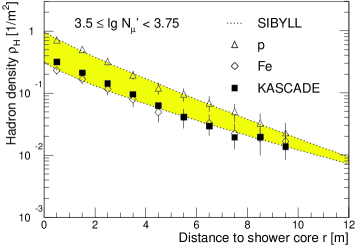
Figure 7: The lateral hadron density for muonic shower sizes corresponding to a mean primary energy of 1.2 PeV. Threshold for hadron detection is 50 GeV. The data are compared with simulations using VENUS (left) and SIBYLL (right), the curves represent fits according to a modified exponential, see text.

Studying hadron distributions at large core distances checks mainly the overall performance of the shower simulation program CORSIKA. In the regions far away from the shower axis of an EAS, the Monte Carlo calculations can be verified with respect to the transport of particles, their decay characteristics, etc. If the hadrons are well described it signifies that the shower propagation is treated properly. In these outer regions, where lower hadron energies and larger scattering angles dominate, the underlying physics is sufficiently well known from accelerator experiments, and the code in itself can be tested.

As an example of such a test, the hadron lateral distribution is presented in Fig. 4 for $N^{\prime}_{\mu}$ sizes corresponding to the primary energy interval around and above the knee: $3~{}\mbox{PeV}\leq E_{0}<10~{}\mbox{PeV}$. The distributions of the number of hadrons and of the hadronic energy are given. In the very centre of the former, a saturation as mentioned in chapter 5 can be noticed. Several functions have been tried to fit the data points, among others exponentials as suggested by Kempa [10]. However, by far the best fit was obtained when applying the NKG formula represented by the curves shown in the graph. This finding is not particularly surprising because hadrons of an energy of approximately 100 GeV [10], when passing through the atmosphere, generate the electromagnetic component, and the NKG formula has been derived for electromagnetic cascades. In addition, multiple scattering of electrons determining the Molière radius resembles the scattering character of hadrons with a mean transverse momentum of 400 MeV/c irrespective of their energy. Replacing the mean multiple scattering by the latter and the radiation length by the interaction length one arrives at a radius $R_{H}$ of about 10 m. This value we expect to take the place of the Molière radius in the NKG formula for electron measurements. Indeed, values of this order are found experimentally.

Lateral hadron distributions compared with CORSIKA simulations are shown in Fig. 5 for primary energies below and above the knee. In the diagrams the hadronic energy density is plotted for muon numbers corresponding to the primary energy intervals of $1~{}\mbox{PeV}\leq E_{0}<3~{}\mbox{PeV}$ and $3~{}\mbox{PeV}\leq E_{0}<10~{}\mbox{PeV}$. The data points are compared to primary proton and iron simulations applying the QGSJET model. These two extreme assumptions about the masses result in nearly identical hadron densities and the measured data coincide with the simulations, thereby verifying the calculations. Similar good agreement is found for the VENUS and SIBYLL models. Simulations and data agree well up to 100 m distance from the core. Only in the very inner region of 10 m, the simulations yield deviating hadron densities for different primary masses. Nevertheless, the measurements here lie well in between the two extreme primary compositions of pure protons or pure iron nuclei.

8 Tests at shower core

8.1 Hadron lateral distribution

To begin with, the lateral distributions are compared with values published in the literature. Hadron distributions in the core of EAS have been measured at Ooty by Vatcha and Sreekantan [11] and at Tien Shan by Danilova et al. [12]. Results of earlier experiments have been examined and discussed by Sreekantan et al. [13]. In the experiments different techniques for hadron detection have been applied: a cloud chamber at Ooty, long gaseous ionisation tubes at Tien Shan and liquid ionisation chambers in the present experiment. Therefore, it is of interest to compare the respective results.

The experiments were performed at different altitudes, and a priori they are expected to deliver deviating results. However, when compared at the same electromagnetic shower size, hadron distributions should be similar because electrons and hadrons, the latter of about 100 GeV, are closely related to each other in an EAS when the shower passes through the atmosphere. A sort of equilibrium turns up as has been pointed out by Kempa [10]. Indeed, Fig. 6 demonstrates for electron numbers $5.25\leq\lg N_{e}<5.5$ that the lateral hadron distributions agree reasonably well. In particular, the measurements of the Ooty group at an atmospheric depth of $800~{}\mbox{g}/\mbox{cm}^{2}$ coincide with the present findings. The grey shaded band represents CORSIKA simulations using the hadronic interaction model QGSJET, the lower curve representing primary protons and the upper curve primary iron nuclei. The curves are fits to the simulated density of hadrons according to $\rho_{H}(r)\propto exp~{}(-(\frac{r}{r_{0}})^{\kappa})$ with values for $\kappa$ found to be between 0.7 and 0.9. The data lie well between these two boundaries. The graph on the righthand side represents hadron densities with a threshold of 1 TeV. Bearing this high threshold in mind, the similarity in both distributions, Tien Shan at $690~{}\mbox{g}/\mbox{cm}^{2}$ and KASCADE at sea–level, is astonishing. In conclusion, it can be stated that hadron densities, despite of being measured with different techniques, agree reasonably well among different experiments.

When classifying hadron distributions according to muonic shower sizes, differences among the interaction models emerge. This becomes apparent in Fig. 7, where the central density is plotted for truncated muon numbers which correspond to a mean energy of about 1.2 PeV. On the left graph, the VENUS calculations enclose the data points leaving the elemental composition to be somewhere between pure proton or pure iron primaries. On the right graph, the measured data points follow the lower boundary of the SIBYLL calculations, suggesting that all primaries are iron nuclei, at this energy obviously an unprobable result.

The lateral distribution demonstrates, and other observables in a similar manner as reported previously [14], that the SIBYLL code generates too low muon numbers thereby entailing a comparison at a different estimate of the primary energy. A hint has already been observed in Fig. 2 where the SIBYLL lines lie above those of QGSJET and VENUS. When hadronic observables are classified according to electromagnetic shower sizes, the disagreement vanishes as will be discussed in the following.

8.2 Hadron energy distribution

Figure 8: Hadron energy distribution for fixed electron number $N_{e}$ corresponding approximately to 6 PeV primary energy. The lines represent CORSIKA simulations with three interaction models, the lower curves for primary iron, the upper for protons.

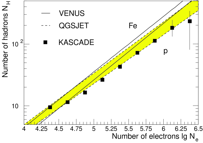
Figure 9: Hadronic shower size vs. electromagnetic shower size. Experimental values are compared with simulations using VENUS (full lines) and QGSJET (shaded area), both for primary protons and iron nuclei. The experimental error bars are rms–values.

The energy distribution of hadrons is shown in Fig. 9 for a fixed electromagnetic shower size. Plotted is the number of hadrons in an area of $8\times 8~{}\mbox{m}^{2}$ around the shower core. As already mentioned, in this way all showers are treated in the same manner, independent of their point of incidence. To avoid a systematic bias the loss in statistics has to be accepted. The number of showers reduces to about 5000. The shower size bin of $5.5\leq\lg N_{e}<5.75$ corresponds approximately to a mean primary energy of 6 PeV. The lines represent fits to the simulations according to $exp~{}(-(\frac{\lg E_{H}-a}{b})^{c})$. Usually in the literature $c=1$ is assumed, however, the present data, due to their large dynamical range, yield values for $c$ from 1.3 to 1.6. As can be inferred from the graph, all three interaction models reproduce the measured data reasonably well, elucidating the fact that electrons closely follow the hadrons in EAS propagation. But if the same data are classified corresponding to the muon number, again SIBYLL seems to generate too many hadrons and thereby mimics a primary composition of pure iron nuclei. For this reason SIBYLL will not be utilized any further. In the figure also the energy spectrum is plotted as measured with the Maket–ANI calorimeter by Ter–Antonian et al. [15]. As already mentioned above, distributions are expected to coincide when taken at the same electron number even if they have been measured at different altitudes. In the present case the data have been taken at sea level and at $700~{}\mbox{g}/\mbox{cm}^{2}$ on Mount Aragats. The energy distributions, indeed, agree rather well with each other indicating that in both data sets the patterns of hadrons are well recognized and the energies correctly determined.

It was seen that SIBYLL encounters difficulties when the data are classified according to muonic shower sizes. The model VENUS, on the other hand, cannot reproduce hadronic observables convincingly well when they are binned into electron number intervals. An example is given in Fig. 9. It shows the number of hadrons, i.e. the hadronic shower size $N_{h}$, as a function of the electromagnetic shower size $N_{e}$. The experimental points match well to the primary proton line as expected from QGSJET predictions. This phenomenon is easily understood by the steeply falling flux spectrum and the fact that primary protons induce larger electromagnetic sizes at observation level than heavy primaries. Hence, when grouping in $N_{e}$ bins , showers from primary protons will be enriched and we expect to have predominantly proton showers in our sample. This fact reduces any ambiguities in the results due to the absence of direct information on primary composition. Concerning the VENUS model the predicted hadron numbers are too high and the two lines which mark the region between primary protons and iron nuclei cannot explain the data. The point at the lowest shower size is still influenced by the trigger efficiency of the array counters.

8.3 Hadron energy fraction

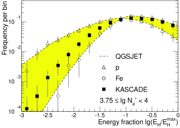
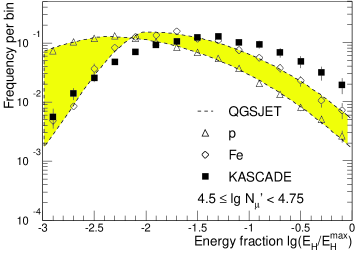
Figure 10: The energy fraction of all hadrons vs. the most energetic hadron in a shower. The data are compared to simulations using the QGSJET model for primary protons (p) and iron nuclei (Fe). Shaded is the physically meaningful region as obtained from the simulations. Primary energies correspond to 2 PeV (left) and 12 PeV (right).

A suitable test of the interaction models consists in investigating the granular structure of the hadronic core concerning spatial as well as energy distributions. As variables we have chosen the energy fraction of hadrons and the distances in the minimum–spanning–tree between them. Both will be dealt with in the following sections.

For each hadron its energy fraction with respect to the most energetic hadron in that particular shower is calculated. For primary protons, the leading particle effect is expected to produce one particularly energetic hadron accompanied by hadrons with a broad distribution of lower energies. Hence, we presume to find a rather large dispersion of hadronic energies for primary protons, whereas for primary iron nuclei the hadron energies should be more equally distributed. The simulated distributions, indeed, confirm this expectation as is shown in Fig. 10. The lines — to guide the eye — represent fits to the simulations using two modified exponentials as in the preceding section, which are connected to each other at the maximum. On the lefthand graph, the data seem to corroborate the simulations. They are shown for a muon number range corresponding to a primary energy of approximately 2 PeV, i.e., below the knee position. On the righthand side, the results are shown for an interval above the knee for muonic shower sizes corresponding to a primary energy of 12 PeV. The reader observes that the data cannot be explained by the simulations, neither by primary protons nor by iron nuclei. On a logarithmic scale the data exhibit a symmetric distribution around the value $\lg(E_{H}/E_{H}^{max})\cong-1.5$, even more symmetric than would be expected for a pure iron composition. In particular, energetic hadrons resulting from the leading particle effect seem to be missing. They would shift the distribution to smaller values. This absence of energetic hadrons in the observations will be confirmed later when investigating other observables.

8.4 Minimum–spanning–tree

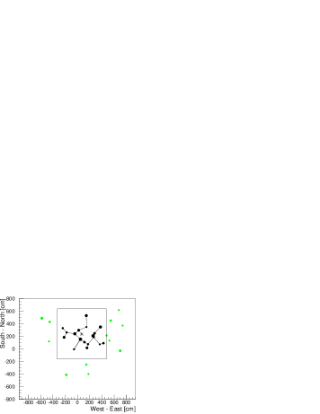
Figure 11: Example of a hadronic core in the calorimeter (top view). The square marks the acceptance area of $8\times 8~{}\mbox{m}^{2}$ around the shower centre (star). The energy of each hadron is indicated by the area of its point in a logarithmic scale.

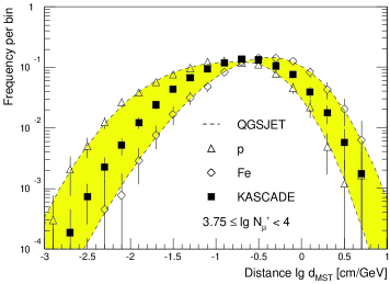
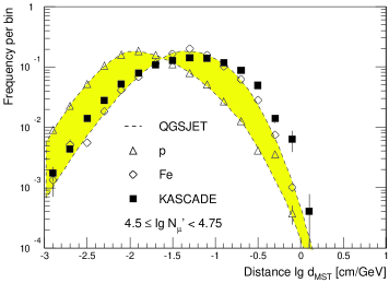
Figure 12: The distances in a minimum–spanning–tree for a muon number interval below (left) and above (right) the knee. The measurements are compared with simulations using the interaction model QGSJET for primary protons (p) and iron nuclei (Fe). The lines are fits to the simulations analogous to Fig. 10.

When constructing the minimum–spanning–tree (MST), all hadrons are connected to each other in a plane perpendicular to the shower axis. The MST is that configuration where the sum of all connections weighted by the inverse energy sum of its neighbours has a minimum. The $1/E$ weighting has been found to separate iron and proton induced showers the most. Fig. 11 shows as an example the central shower core of an event. Plotted are the points of incidence on the calorimeter. The sizes of the points mark the hadron energies on a logarithmic scale. The shower centre and the fiducial area of $8\times 8~{}\mbox{m}^{2}$ around it are indicated as well. For each event the distribution of distances is formed. Average distributions from many events are given in Fig. 12. As in Fig. 10, the muonic shower sizes correspond to primary energy intervals below and above the knee. It is observed that for the former, the data lie well within the bounds of the primary composition but that above the knee the measurements yield results which are not in complete agreement with the model although they are close to the simulated iron data. The distributions of Figs. 10 and 12 have also been calculated analysing the full calorimeter surface and not only the $8\times 8~{}\mbox{m}^{2}$ around the shower centre. No remarkable difference could be obtained.

In both observables – energy fraction and MST – the data for higher primary energies cannot be interpreted by the simulations. Additionally, in the M.C. calculations the knee in the primary energy distribution has been omitted. Again, no remarkable change in the distributions showed up. In fact, when investigating the distributions as a function of muon number, the deviation between M.C. values and the measured data develops smoothly with increasing energy.

When regarding the righthand graph in Fig. 12 the question arises whether the interaction model produces too small distances or too energetic hadrons or both. In agreement with the observation in Fig. 10 one has to conclude that too energetic hadrons are generated as compared to the data. Whether in the MSTs also the distances between the hadrons, in other words the transverse momenta, are underestimated cannot be decided at the moment. Also the number of hadrons plays a role. This issue is under further investigations.

8.5 Hadronic energy in large showers

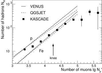
Figure 13: Hadronic shower size vs. muonic shower size (left) and the maximum hadron energy in a shower vs. its muonic shower size (right). The lines represent simulations with the indicated interaction codes. The upper curves represent primary protons, the lower primary iron nuclei.

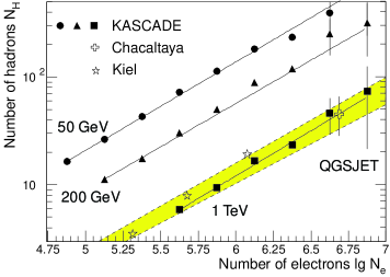
Figure 14: Hadron number at different thresholds, 50 GeV (diamonds), 200 GeV (triangles), and 1 TeV (squares) vs. electromagnetic shower size. The dashed band represents QGSJET simulations for primary protons (lower line) and iron nuclei (upper line).

Deviations between measurement and simulations as in the preceding sections are also observed when investigating the hadronic energy in large showers. With rising muon numbers $N^{\prime}_{\mu}$, the experiment reveals an increasing part of missing hadronic energy in the shower core. Fig. 13 (left) shows the number of hadrons versus the muonic shower size. At muon numbers corresponding to about 5 PeV primary energy, the hadron numbers turn out to be smaller than predicted for iron by both interaction models VENUS and QGSJET. Again, one observes that the latter model describes the experimental points somewhat better. The conclusion that QGSJET reproduces the data best in the PeV region is also confirmed by a recent model comparison performed by Erlykin and Wolfendale [16]. The authors classify the models on the basis of consistency checks among different observables, e.g. the depth of shower maximum $X_{max}$ and the $N_{\mu}/N_{e}$ ratio.

The righthand graph of Fig. 13 presents the maximum hadron energy found in showers with the indicated muon number. The open symbols represent the QGSJET simulations, again QGSJET and VENUS yield similar results. Measurement and simulation disagree also to some extent in this variable at large shower sizes. The overestimation of muon numbers mentioned in section 4 cannot account for the discrepancies. On a logarithmic scale it starts to be noticeable at $\lg N^{\prime}_{\mu}=5.5$ and amounts to $\Delta\lg N^{\prime}_{\mu}=0.1$. A shift of this size does not ameliorate the situation. The data have been checked independently in the reduced fiducial area of $8\times 8~{}\mbox{m}^{2}$. But in this analysis, too, the data seem to fake pure iron primaries at $\lg N^{\prime}_{\mu}=4.3$ and are below that boundary for larger muonic sizes. Factum is that we do not observe the energetic hadrons expected from the M.C. calculations. In the energy region 10 to 100 PeV even QGSJET fails to describe the measurements.

Obviously, the question arises whether these experimentally detected effects are artifacts caused, for instance, by saturation effects in the calorimeter or by insufficient pattern recognition presumed to be different in the simulation than present in the experimental data. After all, the high–energy values correspond to primary energies of about 100 PeV where 400 hadrons have to be reconstructed. At this point, it may be noted again that always the experimental and simulated data are compared with each other on the detector signal level, hence, a possible hadron misidentification applies to both data sets. As already pointed out in section 2, individual hadrons up to 50 TeV have been reconstructed and their saturation effects have been examined thoroughly.

Some misallocation of energy to individual hadrons might occur, though, if lateral distributions of hadrons in the core differ markedly between simulations and reality. There may be indication from emulsion experiments for this [17]. However, from the results shown in Fig. 6 and 7 we would not expect any dramatic effect.

Fig. 14 demonstrates that for large electromagnetic shower sizes, the number of hadrons compares well with other experiments as well as with CORSIKA simulations. In the diagram the number of hadrons above the indicated thresholds is presented with respect to the shower size. The values obtained for hadrons above 1 TeV can be related to two other experiments performed at Kiel by Fritze et al. [18] and on the Chacaltaya by C. Aguirre et al. [19]. It is observed that up to shower sizes which correspond to about 20 PeV for primary protons all high–energy hadrons are reconstructed, i.e., more than 70 TeV energy are found in the calorimeter. When compared to QGSJET simulations, the data lie within the physical boundaries as shown for the 1 TeV line. On closer inspection the data indicate an increase of the mean mass with rising energy. Also in Fig. 9 it has been seen that the hadron numbers are well reproduced by QGSJET up to the highest electromagnetic shower sizes. In conclusion, it can be stated that the hadron component compares well between different experiments and with M.C. calculations when classified according to electromagnetic shower sizes, and that the deviations observed in muon number binning cannot be accounted for by experimental imperfections.

9 Conclusion and outlook

Three interaction models have been tested by examining the hadronic cores of large EAS. It turned out that QGSJET reproduces the data best, but at large muonic shower sizes, i.e. at energies above the knee even this model fails to reproduce certain observables. Most importantly, the model predicts more hadrons than are observed experimentally.

The current investigation is a first approach with a first data sample of the KASCADE experiment. Better statistics, both in the data and in the Monte Carlo calculations, are imperative, especially above the knee in the 10 PeV region, and are expected from the further operation of the experiment. In addition, other experimental methods have to be developed to check the simulation codes even more rigorously. Such a stringent check consists of verifying absolute particle fluxes at ground level at energies where the primary flux is reasonably well known. Improvements in the interaction models are also under way. NEXUS is in statu nascendi, a joint enterprise by the authors of VENUS and QGSJET [20]. It has become evident that a very precise description of the shower development in the atmosphere is needed if the mass of the primaries is to be estimated by means of ground level particle distributions.

10 Acknowledgments

The authors would like to thank the members of the engineering and technical staff of the KASCADE collaboration who contributed with enthusiasm and engagement to the success of the experiment.

The Polish group gratefully acknowledges support by the Polish State Committee for Scientific Research (grant No. 2 P03B 16012). The work has been partly supported by a grant of the Rumanian Ministry of Research and Technology and by the research grant no. 94964 of the Armenian Government and ISTC project A 116. The support of the experiment by the Ministry for Research of the German Federal Government is gratefully acknowledged.

References

References

- [1] D. Heck et al., Report FZKA 6019 (1998) Forschungszentrum Karlsruhe
- [2] H.O. Klages et al., KASCADE Collaboration, Nucl. Phys. B (Proc.Suppl.) 52B (1997) 92
- [3] J. Engler et al., “A Warm–Liquid Calorimeter for Cosmic–Ray Hadrons”, to be published in Nucl. Instr. Meth.
- [4] H.H. Mielke et al., Nucl. Instr. Meth. A360 (1995) 367 and references therein
- [5] K. Werner, Phys. Rep. 232 (1993) 87
- [6] N.N.Kalmykov, S.S.Ostapchenko, Yad. Fiz. 56 (1993) 105; Phys. At. Nucl. 56 (1993) 346; N.N. Kalmykov, S.S. Ostapchenko and A.I. Pavlov, Bull. Russ. Acad. Sci. (Physics) 58 (1994) 1966
-
[7]
J. Engel, T.K. Gaisser, P. Lipari and T. Stanev,
Phys. Rev. D46 (1992) 5013;
R.S. Fletcher, T.K. Gaisser, P. Lipari and T. Stanev, Phys. Rev. D50 (1994) 5710 - [8] GEANT 3.15, Detector Description and Simulation Tool, CERN Program Library Long Writeup W5015, CERN (1993).
- [9] K. Kamata et al., Suppl. Progr. Theor. Phys., 6 (1958) 93
- [10] J. Kempa, Il Nuovo Cimento, 31A (1976) 581
- [11] R.H. Vatcha and B.V. Sreekantan, J. Phys. A: Math., 6 (1973) 1050
- [12] T.V. Danilova et al., Proc. Int. Conf. on Cosmic Rays (La Jolla) 7 (1985) 40
- [13] B.V. Sreekantan et al., Phys. Rev. D 28 (1983) 1050
-
[14]
J.R. Hörandel et al., KASCADE Collaboration,
Proc. Int. Conf. on Cosmic Rays (Durban) 6 (1997) 93;
J.R. Hörandel, Report FZKA 6015 (1998) Forschungszentrum Karlsruhe - [15] S.V. Ter–Antonian et al., Proc. Int. Conf. on Cosmic Rays (Rome), Vol 1 (1995) 369
- [16] A.D. Erlykin and A.W. Wolfendale, Astropart. Phys. 9 (1998) 213
- [17] M. Tamada, Contribution to the Xth Int. Symp. Very High Energy Cosmic Ray Interactions, Gran Sasso, July 1998, proceedings to be published.
- [18] R. Fritze et al., Acta Physica Sc. Hungaricae 29 Suppl. 3 (1969) 439
- [19] C. Aguirre et al., Institute of Cosmic Ray Research, University of Tokyo, Report–434–98–30 (1998) 17
- [20] K. Werner, private communication