The correlation function of X-ray galaxy clusters in the RASS1 Bright Sample

Abstract

We analyse the spatial clustering properties of the RASS1 Bright Sample, an X-ray flux-limited catalogue of galaxy clusters selected from the southern part of the $ROSAT$ All-Sky Survey. The two-point correlation function $\xi(r)$ of the whole sample is well fitted (in an Einstein-de Sitter model) by the power-law $\xi=(r/r_{0})^{-\gamma}$, with $r_{0}=21.5^{+3.4}_{-4.4}\ h^{-1}$ Mpc and $\gamma=2.11^{+0.53}_{-0.56}$ (95.4 per cent confidence level with one fitting parameter). We use the RASS1 Bright Sample as a first application of a theoretical model which aims at predicting the clustering properties of X-ray clusters in flux-limited surveys for different cosmological scenarios. The model uses the theoretical and empirical relations between mass, temperature and X-ray cluster luminosity, and fully accounts for the redshift evolution of the underlying dark matter clustering and cluster bias factor. The comparison between observational results and theoretical predictions shows that the Einstein-de Sitter models display too low a correlation length, while models with a matter density parameter $\Omega_{\rm 0m}=0.3$ (with or without a cosmological constant) are successful in reproducing the observed clustering. The dependence of the correlation length $r_{0}$ on the X-ray limiting flux and luminosity of the sample is generally consistent with the predictions of all our models. Quantitative agreement is however only reached for $\Omega_{\rm 0m}=0.3$ models. The model presented here can be reliably applied to future deeper X-ray cluster surveys: the study of their clustering properties will provide a useful complementary tool to the traditional cluster abundance analyses to constrain the cosmological parameters.

1 Introduction

Galaxy clusters play an important role in the models for structure formation based on the gravitational instability hypothesis. They are the most extended gravitationally bound systems in the Universe. For this reason the study of their properties is a useful tool to constrain the parameters entering in the definition of the cosmological scenarios. In particular, their abundance and spatial distribution (also as a function of redshift) have been used to obtain estimates of the mass fluctuation amplitude and of the density parameter $\Omega_{0}$ (e.g. Eke, Cole & Frenk 1996; Viana & Liddle 1996; Mo, Jing & White 1996; Oukbir, Bartlett & Blanchard 1997; Eke et al. 1998; Sadat, Blanchard & Oubkir 1998; Viana & Liddle 1999; Borgani, Plionis & Kolokotronis 1999; Borgani et al. 1999). In the past years many different groups have compiled deep cluster surveys in the optical band, which have been used to compute the clustering properties of galaxy clusters. The first results showed that clusters are strongly correlated, with a correlation length $r_{0}\approx 20-25\ h^{-1}$ Mpc, a factor 4-5 larger than that obtained for local galaxies (e.g. Bahcall & Soneira 1983; Postman, Huchra & Geller 1992). Here $h$ represents the Hubble constant $H_{0}$ in units of 100 km s^-1 Mpc^-1. Sutherland (1988) suggested the existence of a possible strong effect due to the spurious presence of galaxies acting as interlopers (see also Dekel et al. 1989; van Haarlem, Frenk & White 1997). New analyses of optical catalogues, taking into account this projection effect (Dalton et al. 1992; Nichol et al. 1992; Dalton et al. 1994; Croft et al. 1997), led to a smaller value for the cluster correlation length ($r_{0}\approx 13-18\ h^{-1}$ Mpc).

A way to overcome the projection problem is the use of data obtained in the X-ray region of the spectrum. In fact, in this band, galaxy clusters have a strong emission produced by thermal bremsstrahlung, which allows to detect them also at high redshifts. Starting from the eighties, different space missions produced extended cluster catalogues which have been mainly used to compute their X-ray luminosity function. In particular, the $ROSAT$ satellite provided a good opportunity to build a reliable all-sky survey, which was performed in the soft (0.1 – 2.4 keV) X-ray band. First studies of the clustering properties in small samples of X-ray selected galaxy clusters have been performed by Lahav et al. (1989), Nichol, Briel & Henry (1994) and Romer et al. (1994). More recently the $ROSAT$ data have been correlated with the Abell-ACO cluster catalogue (Abell, Corwin & Olowin 1989) to produce the X-ray Brightest Abell Cluster sample (XBACs; Ebeling et al. 1996), for which estimates of the two-point correlation function have been recently obtained (Abadi, Lambas & Muriel 1998; Borgani, Plionis & Kolokotronis 1999). The corresponding values for $r_{0}$ are in the range $r_{0}\approx 20-26\ h^{-1}$ Mpc. A smaller amplitude of the correlation function is obtained from the preliminary analyses of the REFLEX sample (Collins et al. 1999), which is also obtained by the $ROSAT$ All-Sky Survey (RASS) data.

In this paper we estimate the clustering properties for the RASS1 Bright Sample (De Grandi et al. 1999), which is another X-ray cluster catalogue obtained from the RASS. In this case the clusters are spectroscopically searched in a preliminary list of candidates produced by correlating the X-ray data with regions of galaxy overdensity in the southern sky. In this way, the resulting catalogue is not affected by the selection biases present in the Abell-ACO cluster catalogue. The RASS1 Bright Sample is used to test a theoretical model for the correlation function of X-ray clusters in flux-limited samples (see also Moscardini et al. 1999). This model makes use of the technique introduced by Matarrese et al. (1997) and Moscardini et al. (1998), which allows a detailed modelling of the redshift evolution of clustering, accounting both for the non-linear dynamics of the dark matter distribution and for the redshift evolution of the bias factor. A characteristic feature of this technique is that it takes into full account light-cone effects, which are relevant in analysing the clustering of even moderate redshift objects (see also Matsubara, Suto & Szapudi 1997; de Laix & Starkman 1998; Yamamoto & Suto 1999).

The plan of the paper is as follows. In Section 2 we summarize the characteristics of the RASS1 Bright Sample used in the following clustering analysis. In Section 3 we discuss the method used to compute the observational two-point correlation function for the RASS1 Bright Sample and we present the results. In Section 4 we introduce our theoretical model to estimate the correlations of the X-ray clusters in the framework of different cosmological models and we compare our predictions to the observational results. Conclusions are drawn in Section 5.

2 The Sample

The RASS1 Bright Sample (De Grandi et al. 1999), contains 130 clusters of galaxies selected from the first processing of the $ROSAT$ All-Sky Survey (RASS) data (Voges 1992). This sample was constructed as part of an ESO Key Programme (Guzzo et al. 1995) aimed at surveying all southern RASS candidates, which is now known as the REFLEX cluster survey (Böhringer et al. 1998; Guzzo et al. 1999). The identification of RASS cluster candidates was performed by means of different optically and X-ray based methods. First, candidates were found as overdensities in the galaxy density distribution at the position of the X-ray sources using the COSMOS optical object catalogue (e.g. Heydon-Dumbleton, Collins & MacGillivray 1989). Then, correlating all RASS sources with the ACO cluster catalogue, and, finally, selecting all RASS X-ray extended sources. X-ray fluxes were remeasured using the steepness ratio technique (De Grandi et al. 1997), specifically developed for estimating fluxes from both extended and pointlike objects. A number of selections aimed at improving the completeness of the final sample lead to the RASS1 Bright Sample. Considering the intrinsic biases and incompletenesses introduced by the X-ray flux selection and source identification processes, the overall completeness of the sample is estimated to be $\raise-2.0pt\hbox{\hbox to0.0pt{\hbox{$\sim$}\hss}\raise 5.0pt\hbox{$>$}\ }90$ per cent. The RASS1 Bright Sample is count-rate-limited in the $ROSAT$ hard band (0.5 – 2.0 keV), so that due to the distribution of Galactic absorption its effective flux limit varies between 3.05 and $4\times 10^{-12}$ erg cm^-2 s^-1 over the selected area. This covers a region of approximately 2.5 sr within the Southern Galactic Cap, i.e. $\delta<2.5^{o}$ and $b<-20^{o}$, with the exclusion of patches with RASS exposure times lower than 150 s and of the Magellanic Clouds area. The exact sky map covered by the sample is shown in Figure 2 of De Grandi et al. (1999). The redshift distribution for our whole sample is presented in the left panel of Figure 1 while the X-ray luminosity $L_{X}$ as a function of the redshift for each cluster is shown in the right one. It is possible to notice that 66 per cent of the clusters have $z<0.1$ but the redshift distribution has a tail up to $z\simeq 0.3$.

Figure 1: Left panel: the redshift distribution of the RASS1 Bright Sample. Right panel: the X-ray luminosity $L_{X}$ (in the $ROSAT$ hard band 0.5 – 2.0 keV) vs. the redshift $z$ for each cluster of the sample. The solid line shows the X-ray luminosity corresponding to the limiting flux $S_{\rm lim}=3\times 10^{-12}$ erg s^-1 cm^-2 in an Einstein-de Sitter model.

3 The 2-point correlation function

Before computing the clustering properties of our sample, we have to derive for each cluster the comoving radial distance $r$ from the observer, given the redshift of each source. To this goal we use the standard relation (neglecting the effect of peculiar motions)

$$r(z)={{c}\over H_{0}\sqrt{|\Omega_{0\cal R}|}}{\cal S}\left(\sqrt{|\Omega_{0\cal R}|}\int_{0}^{z}dz^{\prime}\left[\left(1+z^{\prime}\right)^{2}\left(1+\Omega_{\rm 0m}z^{\prime}\right)-z^{\prime}\left(2+z^{\prime}\right)\Omega_{0\Lambda}\right]^{-1/2}\right)\;,$$ (1)

where $\Omega_{0\cal R}\equiv 1-\Omega_{\rm 0m}-\Omega_{0\Lambda}$, with $\Omega_{\rm 0m}$ and $\Omega_{0\Lambda}$ the density parameters for the non-relativistic matter and cosmological constant components, respectively. In this formula, for an open universe model, $\Omega_{0\cal R}>0$ and ${\cal S}(x)\equiv\sinh(x)$, for a closed universe, $\Omega_{0\cal R}<0$ and ${\cal S}(x)\equiv\sin(x)$, while in the Einstein-de Sitter (EdS) case, $\Omega_{0\cal R}=0$ and ${\cal S}(x)\equiv x$.

To compute the spatial two-point correlation function $\xi(r)$ we adopt both the Landy & Szalay (1993) estimator,

$$\xi(r)={{N_{r}(N_{r}-1)}\over{N_{c}(N_{c}-1)}}{{DD(r)}\over{RR(r)}}-{{N_{r}-1}\over{N_{c}}}{{DR(r)}\over{RR(r)}}+1\ ,$$ (2)

and the Davis & Peebles (1983) estimator,

$$\xi(r)=2{{N_{r}}\over{N_{c}-1}}{{DD(r)}\over{RR(r)}}-1\ .$$ (3)

In the previous formulas $N_{r}$ is the number of random points and $N_{c}$ that of clusters, DD is the number of distinct cluster-cluster pairs, DR is the number of cluster-random pairs and RR refers to random-random pairs with separation between $r$ and $r+\Delta r$. The random catalogue contains a number of sources 1,000 times larger than the real catalogue (i.e. $N_{r}=1000N_{c}$). To generate this sample we have extracted randomly coordinates from the surveyed area (see Figure 2 in De Grandi et al. 1999), assigning to each position a random flux drawn from the observed number counts (Figure 8 in De Grandi et al. 1999). We decided to retain the source in the catalogue if its flux is larger than the flux limit at the choosen position. We adopt two different methods to assign the random redshifts: in the first we scramble the observed redshifts of the clusters in the sample; in the second we generate them randomly from the observed redshift distribution binned in intervals of 0.01 in $z$. The results obtained with these two different methods are practically indistinguishable. The same happens also if we use the two previous estimators for the two-point correlation function (eqs.2-3). The errorbars have been estimated by using the bootstrap method with 50 resamplings. We find that the errors obtained in this way are in many cases larger than $\sqrt{3}$ times the Poissonian estimates, which are often used as an analytical approximation of the bootstrap errors (Mo, Jing & Börner 1992). This is particularly true at small separations.

In the left panel of Figure 2 we show the correlation function computed for the whole catalogue. We present results obtained by using both an EdS model and two models with $\Omega_{\rm 0m}=0.3$ (with and without cosmological constant). The results are quite similar and the differences are always small.

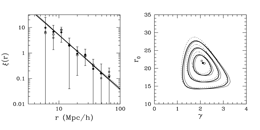
Figure 2: Left panel: the two-point correlation function of the whole RASS1 Bright Sample. Filled circles, open circles and open squares refer to results obtained by assuming $(\Omega_{\rm 0m},\Omega_{0\Lambda})=(1,0)$, $(\Omega_{\rm 0m},\Omega_{0\Lambda})=(0.3,0)$ and $(\Omega_{\rm 0m},\Omega_{0\Lambda})=(0.3,0.7)$, respectively. The corresponding best-fit relations are shown by heavy solid line, light solid line and dotted line, respectively. The 1-$\sigma$ errorbars obtained by the bootstrap method are shown only for the EdS case for clarity; their sizes in the other cases are similar. Right panel: confidence contours (68.3, 95.4 and 99.73 per cent confidence levels) of the fitting parameters $r_{0}$ and $\gamma$ for the two-point correlation function of the whole RASS1 Bright Sample. Heavy solid lines and filled circle refer to confidence levels and to the best fitting value obtained for the EdS case; light solid lines and open circle show the corresponding results for $(\Omega_{\rm 0m},\Omega_{0\Lambda})=(0.3,0)$ while dotted lines and open square refer to $(\Omega_{\rm 0m},\Omega_{0\Lambda})=(0.3,0.7)$ model.

The correlation function has been fitted by adopting the power-law relation

$$\xi(r)=(r/r_{0})^{-\gamma}\ .$$ (4)

The best-fit parameters have been obtained by using a maximum likelihood estimator based on Poisson statistics and unbinned data (Croft et al. 1997; see also Borgani, Plionis & Kolokotronis 1999). Unlike the usual $\chi^{2}$-minimization, this method allows to avoid the uncertainties due to the binsize, to the position of the bin centres and to the bin scale (linear or logarithmic).

To build the estimator, it is necessary to estimate the predicted probability distribution of cluster pairs, given a choice for the correlation length $r_{0}$ and the slope $\gamma$. By using all the distances between the cluster-random pairs, we can compute the number of pairs $g(r)dr$ in arbitrarily small bins $dr$ and use it to predict the mean number of cluster-cluster pairs $h(r)dr$ in that interval as

$$h(r)dr={{N_{c}-1}\over{2N_{r}}}[1+\xi(r)]g(r)dr\ ,$$ (5)

where the correlation function $\xi$ is modelled with a power-law as in eq.(4). Actually the previous equation holds only for the Davis & Peebles (1983) estimator [eq.(3)] but, since we obtain very similar results using different estimators, we can safely apply it here. Now it is possible to use all the distances between the $N_{p}$ cluster-cluster pairs data to build a likelihood. In particular, the likelihood function ${\cal L}$ is defined as the product of the probabilities of having exactly one pair at each of the intervals $dr$ occupied by the cluster-cluster pairs data and the probability of having no pairs in all the other intervals. Assuming a Poisson distribution, one finds

$${\cal L}=\prod_{i}^{N_{p}}\exp[-h(r)dr]h(r)dr\prod_{j\neq i}\exp[-h(r)dr]\ ,$$ (6)

where $j$ runs over all the intervals $dr$ where there are no pairs. It is convenient to define the usual quantity $S=-2\ln{\cal L}$ which can be written, once we retain only the terms depending on the model parameters $r_{0}$ and $\gamma$, as

$$S=2\int^{r_{\rm max}}_{r_{\rm min}}h(r)dr-2\sum_{i}^{N_{p}}\ln[h(r_{i})]\ .$$ (7)

The integral in the previous equation is computed over the range of scales where the fit is made. We will adopt 5 and 80 $h^{-1}$ Mpc for $r_{\rm min}$ and $r_{\rm max}$, respectively.

By minimizing $S$ one can obtain the best-fitting parameters $r_{0}$ and $\gamma$; the confidence levels are defined by computing the increase $\Delta_{S}$ with respect the minimum value of $S$ and assuming a $\chi^{2}$ distribution for $\Delta_{S}$.

By applying this maximum likelihood method to the RASS1 Bright Sample with the assumption of an EdS model, we find $r_{0}=21.5^{+3.4}_{-4.4}\ h^{-1}$ Mpc and $\gamma=2.11^{+0.53}_{-0.56}$ (95.4 per cent confidence level with one fitting parameter). Since the redshift distribution is shallow, the values obtained in other cosmologies are quite similar: for $(\Omega_{\rm 0m},\Omega_{0\Lambda})=(0.3,0)$ we find $r_{0}=21.4^{+3.4}_{-4.6}\ h^{-1}$ Mpc and $\gamma=2.17^{+0.55}_{-0.56}$, while for $(\Omega_{\rm 0m},\Omega_{0\Lambda})=(0.3,0.7)$ we find $r_{0}=22.1^{+3.6}_{-4.7}\ h^{-1}$ Mpc and $\gamma=2.06^{+0.54}_{-0.56}$. The best-fit relations are also shown in Figure 2. Notice that a $\chi^{2}$-minimization procedure gives similar results, but with larger errorbars.

In the right panel of the same figure we show the contour levels corresponding to $\Delta_{S}$ equal to 2.30, 6.31 and 11.8. Assuming that $\Delta_{S}$ is distributed as a $\chi^{2}$ distribution with two degrees of freedom, they correspond to 68.3, 95.4 and 99.73 per cent confidence levels, respectively. Notice that by assuming a Poisson distribution the method considers all pairs as independent, neglecting their clustering. Consequently the resulting errobars can be underestimated (see the discussion in Croft et al. 1997).

Our results are somewhat larger than those derived by Romer et al. (1994) who found $r_{0}=13-15\ h^{-1}$ Mpc by analysing a sample of galaxy clusters also selected from the RASS in a similar region of sky ($22^{h}<$ RA $<3^{h}$, $-50^{o}<\delta<2^{o}$, $|b|>-40^{o}$). A partial explanation of this difference is related to the deeper limiting flux ($S_{\rm lim}\simeq 10^{-12}$ erg s^-1 cm^-2 in the 0.1 – 2.4 keV band) of their catalogue: as we will discuss in the next section, the correlation length is expected to depend on the characteristics defining the surveys, such as their limits in flux and/or luminosity. However we have to remind that this early sample was derived drawing on X-ray information from the $ROSAT$ standard analysis software (SASS), which was not optimazed for the analysis of extended sources (for a more detailed discussion see e.g. De Grandi et al. 1997), and this source of incompleteness was not included in the analysis of Romer et al. (1994). Moreover in their analysis the sample sky coverage (i.e., the surveyed area as a function of the flux limit) was not discussed.

Previous analyses of the XBACs sample, which is a flux-limited catalogue of X-ray Abell clusters with a limiting flux $S_{\rm lim}=5\times 10^{-12}$ erg s^-1 cm^-2 in the 0.1 – 2.4 keV band, gave compatible amplitudes for the correlation function: $r_{0}=21.1^{+1.6}_{-2.3}\ h^{-1}$ Mpc (Abadi, Lambas & Muriel 1998) and $r_{0}=26.0^{+4.1}_{-4.7}\ h^{-1}$ Mpc (Borgani, Plionis & Kolokotronis 1999; errorbars in this case are 2-$\sigma$ uncertainties). Preliminary analyses of the clustering properties of the REFLEX sample (Collins et al. 1999; Guzzo et al. 1999), which has a limiting flux $S_{\rm lim}=3\times 10^{-12}$ erg s^-1 cm^-2 in the 0.1 – 2.4 keV band, lead to a smaller correlation length ($r_{0}\simeq 18\ h^{-1}$ Mpc). Also in this case, the discrepancy is probably a consequence of the deeper limiting flux.

4 Comparison with theoretical models

4.1 Structure formation models

In the following analysis we consider five models, all normalized to reproduce the local cluster abundance. In particular we will adopt the normalizations obtained by Eke, Cole & Frenk (1996) by analysing the temperature distribution of X-ray clusters (Henry & Arnaud 1991). All our models belong to the general class of Cold Dark Matter (CDM) scemarios; their linear power-spectrum can be represented as $P_{\rm lin}(k,0)\propto k^{n}T^{2}(k)$, where, for the CDM transfer function $T(k)$, we use the Bardeen et al. (1986) fit. In particular, we consider three different EdS models, for which the power-spectrum amplitude corresponds to $\sigma_{8}=0.52$ (here $\sigma_{8}$ is the r.m.s. fluctuation amplitude in a sphere of $8h^{-1}$ Mpc). They are: a version of the standard CDM (SCDM) model with shape parameter (see its definition in Sugiyama 1995) $\Gamma=0.45$ and spectral index $n=1$; the so-called $\tau$CDM model, with $\Gamma=0.21$ and $n=1$; a tilted model (TCDM), with $n=0.8$ and $\Gamma=0.41$, corresponding to a high (10 per cent) baryonic content. We also consider an open CDM model (OCDM), with matter density parameter $\Omega_{\rm 0m}=0.3$ and $\sigma_{8}=0.87$ and a low-density flat CDM model ($\Lambda$CDM), with $\Omega_{\rm 0m}=0.3$, with $\sigma_{8}=0.93$. Except for SCDM, which is shown as a reference model, all these models are also consistent with COBE data; for TCDM consistency is achieved by taking into account the possible contribution of gravitational waves to large-angle CMB anisotropies. A summary of the parameters of the cosmological models used in this paper is given in Table 1.

Table 1: The parameters of the cosmological models. Column 2: the present matter density parameter $\Omega_{\rm 0m}$; Column 3: the present cosmological constant contribution to the density $\Omega_{0\Lambda}$; Column 4: the primordial spectral index $n$; Column 5: the Hubble parameter $h$; Column 6: the shape parameter $\Gamma$; Column 7: the spectrum normalization $\sigma_{8}$; Column 8: the value of the parameter $\eta$ in the luminosity-temperature relation required to reproduced the observed $\log N$–$\log S$ (see text for details).

Model	$\Omega_{\rm 0m}$	$\Omega_{0\Lambda}$	$n$	$h$	$\Gamma$	$\sigma_{8}$	$\eta$
SCDM	1.0	0.0	1.0	0.50	0.45	0.52	-0.8
$\tau$CDM	1.0	0.0	1.0	0.50	0.21	0.52	0.0
TCDM	1.0	0.0	0.8	0.50	0.41	0.52	-0.3
OCDM	0.3	0.0	1.0	0.65	0.21	0.87	-0.3
$\Lambda$CDM	0.3	0.7	1.0	0.65	0.21	0.93	-0.2

4.2 The method

Theoretical predictions for the spatial two-point correlation function in the RASS1 Bright Sample have been here obtained in the framework of the above cosmological models by using a method presented in more detail in (Moscardini et al. 1999). Here we only give a short description.

Matarrese et al. (1997; see also Moscardini et al. 1998) developed an algorithm to describe clustering in our past light-cone, where the non-linear dynamics of the dark matter distribution and the redshift evolution of the bias factor are taken into account. In the present paper we adopt a more refined formula which better accounts for the light-cone effects (see Moscardini et al. 1999). The observed spatial correlation function $\xi_{\rm obs}$ in a given redshift interval ${\cal Z}$ is given by the exact expression

$$\xi_{\rm obs}(r)={\int_{\cal Z}dz_{1}dz_{2}{\cal N}(z_{1})r(z_{1})^{-1}{\cal N}(z_{2})r(z_{2})^{-1}~{}\xi_{\rm obj}(r;z_{1},z_{2})\over\bigl{[}\int_{\cal Z}dz_{1}{\cal N}(z_{1})r(z_{1})^{-1}\bigr{]}^{2}}\;,$$ (8)

where $\xi_{\rm obj}(r,z_{1},z_{2})$ is the correlation function of pairs of objects at redshifts $z_{1}$ and $z_{2}$ with comoving separation $r$ and ${\cal N}(z)$ is the actual redshift distribution of the catalogue. A related approach to the study of correlations on the light-cone hypersurface has been recently presented by Yamamoto & Suto (1999) and Nishioka & Yamamoto (1999) within linear theory and by Matsubara, Suto & Szapudi (1997) in the non-linear regime.

An accurate approximation for $\xi_{\rm obj}$ over the scales considered here is

$$\xi_{\rm obj}(r,z_{1},z_{2})\approx b_{\rm eff}(z_{1})b_{\rm eff}(z_{2})\xi_{\rm m}(r,z_{\rm ave})\;,$$ (9)

where $\xi_{m}$ is the dark matter covariance function and $z_{\rm ave}$ is an intermediate redshift between $z_{1}$ and $z_{2}$, for which an excellent approximation is obtained through $D_{+}(z_{\rm ave})=D_{+}(z_{1})^{1/2}D_{+}(z_{2})^{1/2}$ (Porciani 1997), with $D_{+}(z)$ the linear growth factor of density fluctuations.

In our treatment we disregard the effect of redshift-space distortions. Some analytical expressions have been obtained in the mildly non-linear regime, by using either the Zel’dovich approximation (Fisher & Nusser 1996) or higher order perturbation theory (Heavens, Matarrese & Verde 1998). The complicating role of the cosmological redshift-space distortions on the evolution of the bias factor has been considered by Suto et al. (1999). A rough estimate of the effect of redshift-space distortions can be obtained within linear theory and the distant-observer approximation (Kaiser 1987; see Zaroubi & Hoffman 1996 for an extension of this formalism to all-sky surveys). In this case the enhancement of the redshift-space averaged power spectrum is given by the factor $1+2\beta/3+\beta^{2}/5$, where $\beta\simeq\Omega_{\rm 0m}^{0.6}/b_{\rm eff}$ and $b_{\rm eff}$ is the effective bias (see below). Plionis & Kolokotronis (1998), by analysing the XBACs catalogue and using linear perturbation theory to relate the X-ray cluster dipole to the Local Group peculiar velocity, found $\beta\simeq 0.24\pm 0.05$. Adopting this approach, Borgani, Plionis & Kolokotronis (1999) conclude that the overall effect of redshift-space distortions is a small change of the correlation function, which expressed in terms of $r_{0}$ corresponds to an $\simeq 8$ per cent increase.

The effective bias $b_{\rm eff}$ appearing in the previous equation can be expressed as a weighted average of the ‘monochromatic’ bias factor $b(M,z)$ of objects of some given intrinsic property $M$ (like mass, luminosity, …), as follows

$$b_{\rm eff}(z)\equiv{\cal N}(z)^{-1}\int_{\cal M}d\ln M^{\prime}~{}b(M^{\prime},z)~{}{\cal N}(z,M^{\prime})\,,$$ (10)

where ${\cal N}(z,M)$ is the number of objects actually present in the catalogue with redshift in the range $z,~{}z+dz$ and $M$ in the range $M,~{}M+dM$, whose integral over $\ln M$ is ${\cal N}(z)$. In our analysis of cluster correlations we will use for ${\cal N}(z)$ in eq.(8) the observed one, while in the theoretical calculation of the effective bias we will take the ${\cal N}(z,M)$ predicted by the model described below. This phenomenological approach is self-consistent, in that our theoretical model for ${\cal N}(z,M)$ will be required to reproduce the observed cluster abundance and their $\log N$–$\log S$ relation.

For the cluster population it is extremely reasonable to assume that structures on a given mass scale are formed by the hierarchical merging of smaller mass units; for this reason we can consider clusters as being fully characterized at each redshift by the mass $M$ of their hosting dark matter haloes. In this way their comoving mass function $\bar{n}(z,M)$ can be computed using an approach derived from the Press-Schechter technique. Moreover, it is possible to adopt for the monochromatic bias $b(M,z)$ the expression which holds for virialized dark matter haloes (e.g. Mo & White 1996; Catelan et al. 1998). Recently, a number of authors have shown that the Press-Schechter (1974) relation does not provide an accurate description of the halo abundance both in the large and small-mass tails (e.g. Sheth & Tormen 1999). Also, the simple Mo & White (1996) bias formula has been shown not to correctly reproduce the correlation of low mass haloes in numerical simulations. Several alternative fits have been recently proposed (Jing 1998; Porciani, Catelan & Lacey 1999; Sheth & Tormen 1999; Jing 1999). In this paper we adopt the relations recently introduced by Sheth & Tormen (1999), which have been shown to produce an accurate fit of the distribution of the halo populations in the GIF simulations (Kauffmann et al. 1999). They read

$$\bar{n}(z,M)=\sqrt{2aA^{2}\over\pi}\ {{3H_{0}^{2}\Omega_{\rm 0m}}\over{8\pi G}}\ {\delta_{c}\over MD_{+}(z)\sigma_{M}}\ \biggl{[}1+\biggl{(}{{D_{+}(z)\sigma_{M}}\over{\sqrt{a}\delta_{c}}}\biggr{)}^{2p}\biggr{]}\ \bigg{|}{d\ln\sigma_{M}\over d\ln M}\bigg{|}\exp\biggl{[}-{a\delta_{c}^{2}\over 2D_{+}^{2}(z)\sigma^{2}_{M}}\biggr{]}\;$$ (11)

and

$$b(M,z)=1+{1\over\delta_{c}}\biggl{(}{a\delta_{c}^{2}\over\sigma_{M}^{2}D_{+}^{2}(z)}-1\biggr{)}+{2p\over\delta_{c}}\biggl{(}{1\over{1+[\sqrt{a}\delta_{c}/(\sigma_{M}D_{+}(z))]^{2p}}}\biggr{)}\;.$$ (12)

Here $\sigma^{2}_{M}$ is the mass-variance on scale $M$, linearly extrapolated to the present time ($z=0$), and $\delta_{c}$ the critical linear overdensity for spherical collapse. Following Sheth & Tormen (1999), we adopt their best-fit parameters $a=0.707$, $p=0.3$ and $A\approx 0.3222$, while the standard (Press & Schechter and Mo & White) relations are recovered for $a=1$, $p=0$ and $A=1/2$. Notice that

$${\cal N}(z,M)=4\pi r^{2}(z){dr\over dz}\left[1+{H_{0}^{2}\over c^{2}}~{}\Omega_{0\cal R}~{}r^{2}(z)\right]^{-1/2}{\bar{n}}(z,M)~{}\phi(z,M)\;,$$ (13)

where $\phi(z,M)$ is the isotropic catalogue selection function, which also accounts for the catalogue sky coverage, as detailed below.

The last ingredient entering in our computation of the correlation function is the redshift evolution of the dark matter covariance function $\xi_{\rm m}$. As in Matarrese et al. (1997) and Moscardini et al. (1998) we use an accurate method, based on the Hamilton et al. (1991) ansatz, to evolve $\xi_{\rm m}$ into the fully non-linear regime. In particular, we use the fitting formula given by Peacock & Dodds (1996).

In order to predict the abundance and clustering of X-ray clusters in the RASS1 Bright Sample we need to relate X-ray cluster fluxes into a corresponding halo mass at each redshift. The given band flux $S$ corresponds to an X-ray luminosity $L_{X}=4\pi d_{L}^{2}S$ in the same band, where $d_{L}=(1+z)r(z)$ is the luminosity distance. To convert $L_{X}$ into the total luminosity $L_{\rm bol}$ we perform band and bolometric corrections by means of a Raymond-Smith code, where an overall ICM metallicity of $0.3$ times solar is assumed. We translate the cluster bolometric luminosity into a temperature, adopting the empirical relation $T={\cal A}\ L_{\rm bol}^{\cal B}\ (1+z)^{-\eta}$, where the temperature is expressed in keV and $L_{\rm bol}$ is in units of $10^{44}h^{-2}$ erg s^-1. In the following analysis we assume ${\cal A}=4.2$ and ${\cal B}=1/3$; these values allow a good representation of the local data for temperatures larger than $\approx 1$ keV (e.g. David et al. 1993; White, Jones & Forman 1997; Markevitch 1998). Analysing a catalogue of local compact groups, Ponman et al. (1996) showed that at lower temperatures the $L_{\rm bol}-T$ relation has a steeper slope (${\cal B}\approx 0.1$). For these reasons we prefer to fix a minimum value for the temperature at $T=1$ keV. Moreover, even if observational data are consistent with no evolution in the $L_{\rm bol}-T$ relation out to $z\approx 0.4$ (Mushotzky & Scharf 1997), a redshift evolution described by the parameter $\eta$ has been introduced to reproduce the observed $\log N$–$\log S$ relation (Rosati et al. 1998; De Grandi et al. 1999) in the range $2\times 10^{-14}\leq S\leq 2\times 10^{-11}$ (see also Kitayama & Suto 1997; Borgani et al. 1999). The values of $\eta$ required for SCDM, $\tau$CDM, TCDM, OCDM and $\Lambda$CDM models are reported in Table 1. A general discussion of the effects of different choices of the parameters entering in this method (e.g. the scatter in the $L_{\rm bol}-T$ relation) is presented elsewhere (Moscardini et al. 1999).

Finally, with the standard assumption of virial isothermal gas distribution and spherical collapse, it is possible to convert the cluster temperature into the mass of the hosting dark matter halo, namely (e.g. Eke, Cole & Frenk 1996)

$$T={7.75\over\beta_{\rm TM}}{\left(M\over{10^{15}h^{-1}M_{\odot}}\right)}^{2/3}(1+z){\left(\Omega_{\rm 0m}\over\Omega_{\rm m}(z)\right)}^{1/3}\left({\Delta_{\rm vir}(z)\over{178}}\right)^{1/3}\ .$$ (14)

The quantity $\Delta_{\rm vir}$ represents the mean density of the virialized halo in units of the critical density at that redshift (e.g. Bryan & Norman 1998 for fitting formulas). We assume $\beta_{\rm TM}=1.17$, which is in agreement with the results of different hydrodynamical simulations (Bryan & Norman 1998; Gheller, Pantano & Moscardini 1998; Frenk et al. 1999).

Once the relation between observed flux and halo mass at each redshift is established we account for the RASS1 Bright Sample sky coverage $\Omega_{\rm sky}(S)$ (see Figure 7 in De Grandi et al. 1999) by simply setting $4\pi\phi(z,M)=\Omega_{\rm sky}[S(z,M)]$.

4.3 Results

In Figure 3 we compare our predictions for the RASS1 spatial correlation function in different cosmological models to the observational data. All the EdS models here considered predict too small an amplitude. Their correlation lengths are smaller than the observational results: we find $r_{0}\simeq 11.5,12.8,14.8\ h^{-1}$ Mpc for SCDM, TCDM and $\tau CDM$, respectively. On the contrary, both the OCDM and $\Lambda$CDM models are in much better agreement with the data and their predictions are always inside the 1-$\sigma$ errorbars ($r_{0}\simeq 18.4,18.6\ h^{-1}$ Mpc, respectively). In order to quantify the differences between the model predictions and the observational data, we use again the maximum likelihood approach. The minimum value for $S$ is obtained for the $\Lambda$CDM model. A similar value, corresponding to $\Delta_{S}=0.7$, is obtained for the OCDM model, while for the EdS models the resulting $S$ are much larger: $\Delta_{S}=10.6,19.3,26.8$ for $\tau CDM$, TCDM and SCDM models, respectively.

To evaluate what is the effect of neglecting the description of clustering in the past light-cone, as usually done in previous analyses, we estimate the cluster correlation function as $\xi(r)=b^{2}_{\rm eff}(z_{\rm med})\xi_{\rm m}(r,z_{\rm med})$, where $z_{\rm med}$ is the median redshift of the catalogue. For the RASS1 Bright Sample we have $z_{\rm med}\simeq 0.08$. The resulting values of the correlation lengths obtained in this way are $r_{0}\simeq 13.5,15.5,18.2,21.9,22.4\ h^{-1}$ Mpc, for SCDM, TCDM, $\tau CDM$, OCDM and $\Lambda CDM$, respectively. They are typically 20 per cent higher than the estimates obtained by our method. This difference is due to the fact that in the past light-cone formalism the matter correlation functions (and bias factors) are weighted by a factor ${\cal N}(z)/r(z)$, for which the average value on the whole sample corresponds neither to the median nor to the mode of the redshift distribution. Actually, the presence of the comoving radial distance $r(z)$ at the denominator tends to shift the “effective redshift” to smaller values of $z$. As a consequence, the true cluster correlations, which are indeed measured in our past light-cone, have typically smaller amplitudes than those estimated at the median redshift of the catalogue. Of course, the importance of this effect becomes larger when deeper surveys are considered.

Figure 3: Comparison of the observed spatial correlation for clusters in the RASS1 Bright Sample (shown as in Figure 2) with the predictions of the various theoretical models: SCDM (solid line), $\tau$CDM (dotted line), TCDM (short-dashed line), OCDM (long-dashed line) and $\Lambda$CDM (dotted-dashed line).

In order to study the possible dependence of the clustering properties of the X-ray clusters on the observational characteristics defining the survey, we use our model to predict the values of the correlation length $r_{0}$ in catalogues where we vary the limiting X-ray flux $S_{\rm lim}$ or luminosity $L_{\rm lim}$ (both defined in the energy band 0.5 – 2 keV). Notice that this analysis can be related to the study of the richness dependence of the cluster correlation function. In fact, a change in the observational limits implies a change in the expected mean intercluster separation $d_{c}$. Bahcall & West (1992) found that the Abell clusters data are consistent with a linear relation $r_{0}=0.4d_{c}$, while a milder dependence is resulting from the analysis of the APM clusters (Croft et al. 1997). Our results are shown in Figure 4. All the cosmological models display a similar trend: in the flux and luminosity intervals here considered, the correlation length $r_{0}$ has a slow growth with $S_{\rm lim}$ (left panel), and a more marked one with $L_{\rm lim}$ (right panel). For example, for OCDM and $\Lambda CDM$ the correlation length changes from $r_{0}\simeq 18$ to $r_{0}\simeq 21h^{-1}$ Mpc, when the limiting flux varies from $S_{\rm lim}=10^{-12}$ to $S_{\rm lim}=10^{-11}$ erg s^-1 cm^-2, and from $r_{0}\simeq 18$ to $r_{0}\simeq 30h^{-1}$ Mpc, when the limiting luminosity varies from $L_{\rm lim}=10^{42}$ to $L_{\rm lim}=10^{44}h^{-2}$ erg s^-1. The values of $r_{0}$ for the EdS models have similar variations but are always smaller. We can compare these predictions to the results obtained by computing the two-point correlation function in the RASS1 Bright Sample with the same cuts in X-ray flux or luminosity. The estimates of $r_{0}$ obtained in this way are presented in Table 2 (where we also report the number of clusters inside each subsample) and shown in the figure (open squares). In both panels the whole catalogue is represented by the square on the right. Because of the small number of clusters in these subsamples, we prefer to fit the correlation function by fixing the value of the slope $\gamma=1.8$; we find that our values of $r_{0}$ are only slightly dependent on this assumption. The errorbars shown in the figure correspond to an increase $\Delta_{S}=4$ with respect to the minimum value of $S$. With the assumption that $\Delta_{S}$ is distributed as a $\chi^{2}$ distribution with a single degree of freedom, this corresponds to 95.4 per cent confidence level. By analysing the trend with changing limiting flux, we find that the observed values of $r_{0}$ are almost constant even if $S_{\rm lim}$ changes by a factor larger than 2. This result is in agreement with what Borgani, Plionis & Kolokotronis (1999) obtained for XBACs. We notice that OCDM and $\Lambda$CDM are able to reproduce the amount of clustering shown by the RASS1 Bright Sample, while all the EdS models strongly underpredict the amplitude of the correlation function. The situation is slightly different when we analyse luminosity-limited catalogues. The RASS1 Bright Sample suggests a small increase of $r_{0}$ with $L_{\rm lim}$, even if the hypothesis of a constant correlation length cannot be rejected. This is consistent with a similar analysis made by Abadi, Lambas & Muriel (1998) on the XBACs catalogue. As shown in the left panel of Figure 4, our models always tend to predict smaller correlations, even if the non-EdS models are still marginally consistent with the observational data.

Figure 4: The behaviour of the correlation length $r_{0}$ as a function of the limiting X-ray flux $S_{\rm lim}$ (left panel) and luminosity $L_{\rm lim}$ (right panel). The open squares and errorbars (95.4 per cent confidence level) refer to different subsamples of RASS1 Bright Sample here analysed. The prediction of the various theoretical models are shown as in Figure 3: SCDM (solid line), $\tau$CDM (dotted line), TCDM (short-dashed line), OCDM (long-dashed line) and $\Lambda$CDM (dotted-dashed line).

Table 2: The correlation length $r_{0}$ in flux-limited (left) and luminosity-limited (right) subsamples of the RASS1 Bright Sample. Column 1: the limiting X-ray flux $S_{\rm lim}$ (in units of $10^{-11}$ erg s^-1 cm^-2) or luminosity $L_{\rm lim}$ (in units of $10^{44}h^{-2}$ erg s^-1); Column 2: the number of clusters in the subsample; Column 3: the correlation length $r_{0}$ (in units of $h^{-1}$ Mpc) as obtained from the maximum likelihood analysis with fixed slope $\gamma=1.8$ (errorbars correspond to 95.4 per cent confident level)

$S_{\rm lim}$	no. of clusters	$r_{0}$		$L_{\rm lim}$	no. of clusters	$r_{0}$
0.3	126	$21.2^{+4.0}_{-4.1}$		0.01	126	$21.2^{+4.0}_{-4.1}$
0.5	78	$23.7^{+5.2}_{-5.4}$		0.03	122	$22.6^{+4.2}_{-4.2}$
0.7	41	$18.1^{+9.3}_{-11.1}$		0.05	118	$23.1^{+4.3}_{-4.3}$
				0.10	115	$24.3^{+4.4}_{-4.5}$
				0.15	106	$24.9^{+5.1}_{-5.4}$
				0.20	98	$27.2^{+6.0}_{-6.1}$
				0.25	89	$30.2^{+7.1}_{-7.2}$
				0.30	84	$32.5^{+7.6}_{-7.7}$
				0.40	74	$32.8^{+9.5}_{-9.9}$

5 Conclusions

In this paper we have studied the two-point correlation function $\xi(r)$ of a flux-limited sample of X-ray galaxy clusters, the RASS1 Bright Sample. These observational results have been used to test a theoretical model predicting the clustering properties of X-ray clusters in flux-limited surveys in the framework of different cosmological scenarios. Our main results are:

• Assuming an Einstein-de Sitter model, $\xi(r)$ can be well fitted using the standard power-law relation $\xi=(r/r_{0})^{-\gamma}$, with $r_{0}=21.5^{+3.4}_{-4.4}h^{-1}$ Mpc and $\gamma=2.11^{+0.53}_{-0.56}$ (95.4 per cent confidence levels with one fitting parameter). The values obtained in models with matter density parameter $\Omega_{\rm 0m}=0.3$ are quite similar.

• The amplitude of the correlation function is almost constant when the RASS1 Bright Sample is analysed with different limiting fluxes in the range $S_{\rm lim}=3-7\times 10^{-12}$ erg s^-1 cm^-2 while it displays a slightly increasing trend when computed in catalogues with an increasing X-ray luminosity limit in the range $L_{\rm lim}=0.01-0.4\times 10^{44}h^{-2}$ erg s^-1.

• The comparison with the predictions of our theoretical models shows that the Einstein-de Sitter models are unable to reproduce the observational results obtained for the whole RASS1 Bright Sample. On the contrary, good agreement is found for the models with matter density parameter $\Omega_{\rm 0m}=0.3$, both with and without a cosmological constant.

• Our models are also able to reproduce the behaviour of $r_{0}$ with $S_{\rm lim}$ and $L_{\rm lim}$, but the observed amount of clustering is reproduced only by the open and $\Lambda$ models.

In conclusion, we believe that the method presented here leads to robust predictions on the clustering of X-ray clusters; its future application to new and deeper catalogues will allow to provide useful constraints on the cosmological parameters.

References

- [] Abadi M.G., Lambas D.G., Muriel H., 1998, ApJ, 507, 526
- [] Abell G.O., Corwin H.G., Olowin R.P., 1989, ApJS, 70, 1
- [] Bahcall N.A., Soneira R.M., 1983, ApJ, 270, 20
- [] Bahcall N.A., West M., 1992, ApJ, 392, 419
- [] Bardeen J.M., Bond J.R., Kaiser N., Szalay A.S., 1986, ApJ, 304, 15
- [] Bohringer H. et al., 1998, Messanger, 94, 21
- [] Borgani S., Plionis M., Kolokotronis V., 1999, MNRAS, 305, 866
- [] Borgani S., Rosati P., Tozzi P., Norman C., 1999, ApJ, 517, 40
- [] Bryan G.L., Norman M.L., 1998, ApJ, 495, 80
- [] Catelan P., Lucchin F., Matarrese S., Porciani C., 1998, MNRAS, 297, 692
- [] Collins C.A. et al., 1999, in preparation
- [] Croft R.A.C., Dalton G.B., Efstathiou G., Sutherland W.J., Maddox S.J., 1997, MNRAS, 291, 305
- [] Dalton G.B., Croft R.A.C., Efstathiou G., Sutherland W.J., Maddox S.J., Davis M., 1994, MNRAS, 271, L47
- [] Dalton G.B., Efstathiou G., Maddox S.J., Sutherland W.J., 1992, ApJ, 390, L1
- [] David L.P., Slyz A., Jones C., Forman W., Vrtilek S.D., Arnaud K.A., 1993, ApJ, 412, 479
- [] Davis M., Peebles P.J.E., 1983, ApJ, 267, 465
- [] De Grandi S., Molendi S., Böhringer H., Chincarini G., Voges W., 1997, ApJ, 486, 738
- [] De Grandi S. et al., 1999, ApJ, 514, 148
- [] Dekel A., Blumenthal G.R., Primack J.R., Olivier S., 1989, ApJ, 338, L5
- [] de Laix A.A., Starkman G., 1998, ApJ, 501, 427
- [] Ebeling H., Voges W., Boheringer H., Edge A.C., Huchra J.P., Briel U.G., 1996, MNRAS, 283, 1103
- [] Eke V.R., Cole S., Frenk C.S., 1996, MNRAS, 282, 263
- [] Eke V.R., Cole S., Frenk C.S., Henry P.J., 1998, MNRAS, 298, 1145
- [] Fisher K.B., Nusser A., 1996, MNRAS, 279, L1
- [] Frenk C.S. et al., 1999, ApJ, 525, 554
- [] Gheller C., Pantano O., Moscardini L., 1998, MNRAS, 296, 85
- [] Guzzo L. et al., 1995, in Wide Field Spectroscopy and Distant Universe, Maddox S. J. & Aragon-Salamanca A. (eds), World Scientific, 205
- [] Guzzo L. et al., 1999, Messanger, 95, 27
- [] Hamilton A.J.S., Kumar P., Lu E., Mathews A., 1991, ApJ, 374, L1
- [] Heavens A.F., Matarrese S., Verde L., 1998, MNRAS, 301, 797
- [] Henry J.P., Arnaud K.A., 1991, ApJ, 372, 410
- [] Heydon-Dumbleton N.H., Collins C.A., MacGillivray H.T., 1989, MNRAS, 238, 379
- [] Jing Y.P., 1998, ApJ, 503, L9
- [] Jing Y.P., 1999, ApJ, 515, L45
- [] Kaiser N. 1987, MNRAS, 227, 1
- [] Kauffmann G., Colberg J.M., Diaferio A., White S.D.M., 1999, MNRAS, 303, 188
- [] Kitayama T., Suto Y., 1997, ApJ, 490, 557
- [] Lahav O., Fabian A.C., Edge A.C., Putney A., 1989, MNRAS, 238, 881
- [] Landy S.D., Szalay A.S., 1993, ApJ, 412, 64
- [] Markevitch M., 1998, ApJ, 504, 27
- [] Matarrese S., Coles P., Lucchin F., Moscardini L., 1997, MNRAS, 286, 115
- [] Matsubara T., Suto Y., Szapudi I., 1997, ApJ, 491, L1
- [] Mo H.J., Jing Y.P., Börner G., 1992, ApJ, 392, 452
- [] Mo H.J., Jing Y.P., White S.D.M., 1996, MNRAS, 282, 1096
- [] Mo H.J., White S.D.M., 1996, MNRAS, 282, 347
- [] Moscardini L., Coles P., Lucchin F., Matarrese S., 1998, MNRAS, 299, 95
- [] Moscardini L., Matarrese S., Lucchin F., Rosati P., 1999, preprint, astro-ph/9909273
- [] Mushotzky R.F., Scharf C.A., 1997, ApJ, 482, L13
- [] Nichol R.C., Briel O.G., Henry J.P., 1994, MNRAS,267, 771
- [] Nichol R.C., Collins C.A., Guzzo L., Lumsden S.L., 1992, MNRAS, 255, 21p
- [] Nishioka H., Yamamoto K., 1999, ApJ, 520, 426
- [] Oubkir J., Bartlett J.G., Blanchard A., 1997, A&A, 320, 365
- [] Peacock J.A., Dodds S.J., 1996, MNRAS, 280, L19
- [] Plionis M., Kolokotronis V., 1998, ApJ, 500, 1
- [] Ponman T.J., Bourner P.D.J., Ebeling H., Böringer H., 1996, MNRAS, 283, 690
- [] Porciani C., 1997, MNRAS, 290, 639
- [] Porciani C., Catelan P., Lacey C., 1999, ApJ, 513, L99
- [] Postman M., Huchra J.P., Geller M.J., 1992, ApJ, 384, 404
- [] Press W.H., Schechter P., 1974, ApJ, 187, 425
- [] Romer A.K., Collins C.A., Böhringer H., Cruddace R.C., Ebeling H. MacGillawray H.T., Voges W., 1994, Nat, 372, 75
- [] Rosati P., Della Ceca R., Norman C., Giacconi R., 1998, ApJ, 492, L21
- [] Sadat R., Blanchard A., Oubkir J., 1998, A&A, 329, 21
- [] Sheth R.K., Tormen G., 1999, MNRAS, 308, 119
- [] Sugiyama N., 1995, ApJS, 100, 281
- [] Sutherland W.J., 1988, MNRAS, 234, 159
- [] Suto Y., Magira H., Jing Y.P., Matsubara T., Yamamoto K., 1999, Prog. Theor. Phys. Suppl., 133, 183
- [] van Haarlem M.P., Frenk C.S., White S.D.M., 1997, MNRAS, 287, 817
- [] Viana P.T.P., Liddle A.R., 1996, MNRAS, 281, 323
- [] Viana P.T.P., Liddle A.R., 1999, MNRAS, 303, 535
- [] Voges W., 1992, in Proceedings of Satellite Symposium 3, ed. T. D. Guyenne & J. J. Hunt, ESA-ISY-3 (Noordwijk:ESA), 9
- [] White D.A., Jones C., Forman W., 1997, MNRAS, 292, 419
- [] Yamamoto K., Suto Y., 1999, ApJ, 517, 1
- [] Zaroubi S., Hoffman Y., 1996, ApJ, 462, 25