Observational Signatures of the First Luminous Objects

Abstract

The next generation of astronomical instruments will be able to detect dense pockets of ionized gas created by the first luminous objects. The integrated free-free emission from ionized halos creates a spectral distortion of the Cosmic Microwave Background, greater than the distortion due to the reionized intergalactic medium. Its detection is well within the capabilities of the planned DIMES satellite. Ionized halos may also be imaged directly in free-free emission by the Square Kilometer Array. Bright halos will be detected as discrete sources, while residual unresolved sources can still be detected statistically from temperature fluctuations in maps. Balmer line emission from ionized halos is detectable by the Next Generation Space Telescope and can be used to obtain redshift information. Unlike Ly$\alpha$, the H$\alpha$ line does not suffer from resonant scattering by neutral hydrogen, and is still observable when the IGM is not fully reionized. In addition, it is less susceptible to dust extinction. Finally, the kinetic Sunyaev-Zeldovich effect may be used to detect ionized gas at high redshift. Used in concert, these observations will probe ionizing emissivity, gas clumping, and star formation in the early universe.

1 Introduction

Stimulated in part by the upcoming launches of the next generation of astronomical instruments, the epoch of reionization has become the subject of increasingly intense theoretical effort in recent years. Reionization affects observations of the Cosmic Microwave Background, both as a source of new anisotropies, and in suppressing small-scale fluctuations from the surface of last scatter (Haiman & Knox, 1999, and references therein). In addition, the Next Generation Space Telescope (NGST) offers the prospect of directly detecting the first luminous objects. Nonetheless, the large number of complex, non-linear physical processes involved means that it is extremely difficult to make firm theoretical predictions with any kind of confidence. While it appears quite likely that NGST will be able to image Population III objects in the infrared continuum (Haiman & Loeb 1997, 1998), and detection of the Gunn-Peterson trough may yield the redshift at which the IGM is not yet fully reionized (Miralda-Escude & Rees 1998), this information alone falls far short of being able to fully constrain models of reionization. Key among the uncertainties is the ionizing emissivity of collapsed objects, and the degree of gas clumping. In this paper, we suggest the observation of diffuse gas and Population III objects in thermal bremstrahhlung and recombination line emission as a direct probe of these quantities. Due to their $n_{e}^{2}$ dependence, free-free and recombination line fluctuations trace the clumpiness and ionization fraction of the gas. While the intensities of these signals are directly proportional to one another, their joint detection should prove invaluable, given the highly different nature of the foreground contaminants and instrumental systematics in each case. In addition, we examine the prospects for detecting ionized gas at high redshift via the kinetic Sunyaev-Zeldovich effect. Below, we briefly summarize the observational case for each signal.

Balmer line emission Discussion in the literature on detecting line emission from high redshift galaxies has thus far focussed predominantly on Ly$\alpha$ (Miralda-Escude & Rees 1998, Kunth et al 1998). However, detection in Ly$\alpha$ faces problems due to attenuation by dust and resonant scattering by neutral hydrogen. Indeed, in the dark ages before the universe was completely reionized, it is unlikely that we will be able to detect sources in Ly$\alpha$ emission, due to the large column density of neutral hydrogen along the line of sight. By contrast, Balmer lines face none of these problems, and provide a much cleaner probe of ionizing emissivities. Thus, for instance, the intensity of H$\alpha$ emission is intimately linked to star formation rates. In this paper, we show that for equivalent integration times with NGST, moderate resolution spectroscopy (${\rm R\sim 1000}$) should yield H$\alpha$ line detection with the same signal to noise as continuum IR imaging for $z<6.6$, and 10% signal to noise compared to IR imaging for $z>6.6$. Thus, if a high-redshift galaxy is detected in imaging mode, H$\alpha$ line detection should be eminently feasible. In addition, higher order Balmer lines such as H$\beta$ should also be detectable. The redshift information provided by Balmer line emission should provide an invaluable complement to free-free and IR imaging.

Free-free emission In addition to Compton scattering off hot gas via the Sunyaev-Zeldovich effect, free-free emission from the ionized IGM can also produce a spectral distortion of the CMB (Barlett & Stebbins 1991). This distortion increases quadratically at low frequencies, and is poorly constrained by COBE observations near the peak of the CMB spectrum ($\nu\sim 56$ GHz). One of the drivers behind the development of the DIMES satellite (Kogut et al 1996; see http://ceylon.gsfc.nasa.gov/DIMES) is the hope of detecting this distortion produced by the ionized IGM at low frequencies ($\nu\sim 2$ GHz). The magnitude of the distortion is directly related to the optical depth of ionized gas in the IGM, and thus has the potential to constrain the epoch of reionization. However, the ionized IGM is not the only source of free-free emission. Lyman limit systems in ionization equilibrium with the external intergalactic ionizing background emit thermal bremsstrahlung radiation (Loeb 1996), as do ionized halos with an internal source of ionizing radiation (Haiman & Loeb 1997). In this paper, we argue that if the escape fraction of ionizing photons from starburst galaxies is small (as is indicated by local observations), then the integrated contribution of ionized halos to the free-free background overwhelms that of the IGM, regardless of the details of the reionization history of the universe. Thus, the detection of a spectral distortion by DIMES is likely to probe the integrated ionizing emissivity and clumping of gas in halos, rather than the optical depth of the reionized IGM.

A natural way to tell if an observed spectral distortion is produced by ionised halos rather than an ionised IGM is to observe fluctuations in the free-free background. If the spectral distortion of the CMB is produced by the IGM, it should exhibit a fairly smooth spatial signature across the sky, whereas if ionized halos predominate then the free-free background should exhibit a great deal of small scale power. Since Galactic foregrounds in free-free and synchrotron emission damp rapidly at small scales, it should be possible to directly image the predicted population of high redshift ionized halos with a high resolution instrument. This is an application well suited for the proposed Square Kilometer Array, or SKA (Braun et al 1998) which will operate in the frequency range $0.03-20$ GHz with an angular resolution comparable to that of HST ($\sim 0.1^{\prime\prime}$) and a sensitivity 100 times better than the VLA, down to the $\sim 20$ nJy level. Such a quantum leap in performance should reap immense scientific rewards.

At present, the appearance of the radio sky at nano Jansky levels is not known. We make a first stab at characterising observable properties of a predicted population of free-free emitters. In our Press-Schechter based model, we find that $\sim 10^{4}$ sources at $z>5$ should be directly detectable as discrete sources in the $1^{\circ}$ SKA field of view. In addition, the integrated background from sources too faint to be directly identified creates a fluctuating signal, similar to the Extragalactic Background Light (EBL) in the optical and the Cosmic Infrared Background (CIB) in the IR, which may be characterised by its power spectrum and skewness. Finally, we investigate the clustering of sources at high redshift and find that while it is fairly substantial, the observed signal is still likely to be dominated by Poisson fluctuations.

In all numerical estimates, we assume a background cosmology given by the ’concordance’ values of Ostriker & Steinhardt (1995): $(\Omega_{m},\Omega_{\Lambda},\Omega_{b},h,\sigma_{8h^{-1}},n)=(0.35,0.65,0.04,0.65,0.87,0.96)$. We use expressions from Carroll, Press & Turner (1992) and Eisenstein (1997) to compute cosmological expressions such as the growth factor and luminosity distance.

2 Modelling the Ionizing Sources

2.1 Estimating Halo Luminosities

Since the free-free and H$\alpha$ emissivity are both proportional to $\langle n_{e}^{2}\rangle$, observational prospects hinge crucially on this quantity at high redshift. The signal is dominated by the small-scale clumping of the gas at high redshift. One approach to estimating $\langle n_{e}^{2}\rangle$ is to model the properties of halos at high redshift. It is not known to what extent the baryons can cool and condense in halos at high redshift. A minimal assumption would be that gas within a halo traces the distribution of the dark matter, generally overdense by $\delta\sim 180$ at collapse; this would indicate $\langle n_{e}^{2}\rangle\propto(1+z)^{6}$. Observations of the local universe indicate that the maximum luminosity density of dynamically hot stellar systems varies as $M^{-4/3}$(Burstein et al 1997), which implies that the gas is more centrally condensed in low mass systems (which are prevalent at high redshift), presumably because dissipational effects are more efficient. Thus, the above scaling with redshift is likely an underestimate. If the gas settles to form a disk it could be overdense by $\delta\sim 18\pi^{2}\lambda^{-3}\sim 10^{6}$ (Dalcanton, Spergel & Summers 1997), where the spin parameter $\lambda\sim 0.05$ typically (Barnes & Efstathiou 1987). Note, however that $\langle n_{e}^{2}\rangle$ is likely to be dominated by the local clumping of the ISM in ionization bounded HII regions (in other words, the clumping factor $\langle n_{e}^{2}\rangle/\langle n_{e}\rangle^{2}$ of the gas is significantly greater than unity), in which case these limits would have to be revised upwards.

A simpler and likely more accurate approach is to assume that most of the ionizing radiation produced is absorbed locally in the halo, with only a small fraction escaping ($<20\%$). This is consistent with our observations of the nearby universe. For instance, the observation of 4 starburst galaxies with the Hopkins Ultraviolet Telescope (HUT) by Leitherer et al (1995) report an escape fraction of only $3\%$, by comparing the observed Lyman continuum flux with that predicted from theoretical spectral energy distributions. In our own galaxy, the models of Dove, Shull & Ferrara (1999) have an escape fraction for ionizing photons of $6\%$ and $3\%$ (for coeval and Gaussian star formation histories respectively) from OB associations in the Milky Way disk, while Bland-Hawthorn & Maloney (1999) find an escape fraction of $6\%$ is necessary for consistency with the observed line emission from the Magellanic stream and high velocity clouds. The increasing density of the gas in halos with collapse redshift indicates that the escape fraction should decrease, strengthening our bound. The production rate of recombination line photons $\dot{N}_{\rm recomb}$ is directly related to the production rate of ionizing photons:

$$\dot{N}_{\rm recomb}=\alpha_{B}\langle n_{e}^{2}\rangle V\approx(1-f_{esc})\dot{N}_{\rm ion}$$ (1)

where $\dot{N}_{\rm ion}$ is the number of ionizing photons emitted per second, and $\alpha_{B}$ is the case B recombination coefficient.

In this manner the luminosities of a source in H$\alpha$ and free-free emission scale directly with the production rate of ionizing photons. For H$\alpha$, Hummer & Storey (1987) find that 0.45 H$\alpha$ photons are emitted per Lyman continuum photon over a wide range of nebulosity conditions. We thus obtain directly

$${\rm L(H\alpha)}=1.4\times 10^{41}\left(\frac{\dot{N}_{\rm ion}}{10^{53}{\rm photons\,s^{-1}}}\right){\rm ergs\,s^{-1}}.$$ (2)

For free-free emission, the volume emissivity for a plasma is (Rybicki & Lightman 1979):

$$\epsilon_{\nu}=3.2\times 10^{-39}n_{e}^{2}\left(\frac{T}{10^{4}K}\right)^{-0.35}\ {\rm erg\,s^{-1}\,cm^{-3}\,Hz^{-1}}$$ (3)

where we adopt the velocity averaged Gaunt factor $\bar{g}_{ff}=4.7$ and approximate its mild temperature dependence with a power law. We can then use the estimate of $n_{e}^{2}V$ derived from equation (1) to obtain:

$$L_{\nu}^{ff}=1.2\times 10^{27}\left(\frac{\dot{N}_{\rm ion}}{10^{53}{\rm photons\,s^{-1}}}\right){\rm ergs\,s^{-1}\,Hz^{-1}}$$ (4)

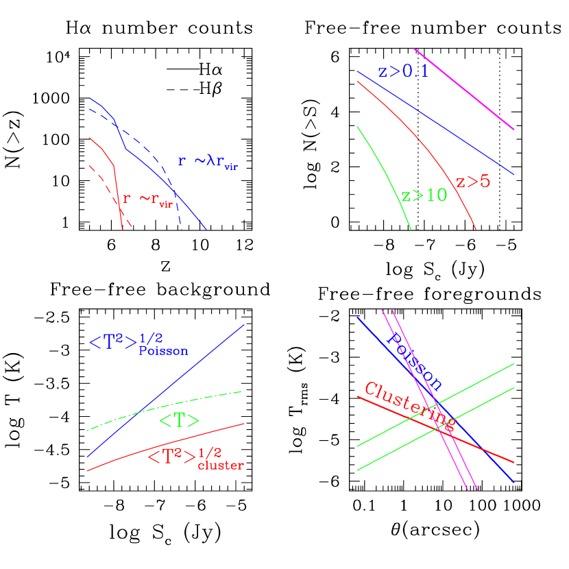
Figure 7: Figures (2) (H$\alpha$ number counts),(3) (Free-free number counts), (4) (Free-free background),(6) (Free-free foregrounds), computed for the lower star formation efficiency case $f_{star}=1.7\%$. All other assumptions are unchanged.

We thus wish to estimate $\dot{N}_{\rm ion}(M)$, the production rate of ionizing photons as a function of halo mass. We can either assume that this function is independent of collapse redshift, or that it evolves with redshift. In this paper, we adopt the models of Haiman & Loeb (1998), which assume the former. In particular, we adopt their starburst model, which is normalised to the observed metallicity $10^{-3}Z_{\odot}\leq Z\leq 10^{-2}Z_{\odot}$ of the IGM at $z\sim 3$. In this model, a constant fraction of the gas mass turns into stars, $1.7\%\leq f_{star}\leq 17\%$ in a starburst which fades after $\sim 10^{7}$ years. In this paper, we shall assume the upper value $Z\sim 10^{-2}Z_{\odot}$, corresponding to $f_{star}\sim 17\%$, in our discussion and plots. We show the results of the calculations for the lower limit star formation efficiency $f_{star}\sim 1.7\%$ in figure (7) (discussed in section (4.2.6)). During the starburst period, the rate of production of ionizing photons is:

$$\dot{N}_{\rm ion}(M)=2\times 10^{53}\,(f_{star}/0.17)\,(M/10^{9}M_{\odot})\,{\rm photons}\,{\rm s^{-1}}$$ (5)

Their mini-quasar model yields similar estimates, $\dot{N}_{\rm ion}(M)=4\times 10^{53}(M/10^{9}M_{\odot})$photons ${\rm s^{-1}}$, with the quasar fading after $\sim 10^{6}$ yrs. The quasar model is normalised to the observed quasar luminosity function at low redshift, assuming a constant ratio of black hole mass to halo mass. We consider the adopted model to be a reasonably conservative estimate for high redshift sources, as it seems quite possible that the efficiency of ionizing photon production increases with redshift. The star formation rate is tied to the dynamical timescale of the gas, SFR$\propto M_{g}/t_{dyn}$. Since high redshift sources are denser, the free-fall time is shorter and $\dot{N}_{ion}\propto{\rm SFR}\propto(1+z)^{1.5}$. Alternatively, one can use the empirical Schmidt law SFR$\propto\Sigma_{g}^{1.4}$ (Kennicutt 1998), where $\Sigma_{g}$ is the gas surface density, in conjunction with an isothermal sphere model to deduce $\dot{N}_{ion}\propto{\rm SFR}\propto(1+z)^{0.8}$ (all scalings are for an object of fixed collapse mass). Intriguingly, Weedman et al (1998) find from observations of galaxies in the HDF that high redshift starbursts have intrinsic UV surface brightnesses typically four times brighter than low redshift starbursts. Furthermore, the absence of metals to provide cooling in the early universe would tend to lead to a top-heavy IMF (Larson 1998), further increasing the efficiency of ionizing photon production. Note also that in our adopted model the escape fraction should fall with redshift, since $\dot{N}_{\rm ion}$ is independent of redshift, whereas $\dot{N}_{\rm recomb}\propto\langle n_{e}^{2}\rangle V\propto(1+z)^{3}$ (using $r_{vir}\propto(1+z)^{-1}$).

We pause to note the possible caveat that supernovae could drive gas out of the galaxy (Dekel & Silk 1986), thereby drastically increasing the escape fraction of ionizing photons and vitiating our assumptions. The expulsion of gas would also shut off further star formation. Although there is enough energy from supernovae to drive such a wind, recent numerical simulations (Mac Low & Ferrara 1999) indicate that mass ejection is in fact only efficient in galaxies with $M_{g}<10^{6}M_{\odot}$ (such galaxies are excluded from our analysis), where the small depth of the potential well means that gas is extremely easily unbound. In higher mass galaxies, the supernovae produce a hole in the interstellar medium through which the shock heated gas is expelled, while the cold gas remains bound. We thus ignore the effect of gas expulsion by supernovae. Note also that our emissivities are calibrated to a quiescent, steady-state mode of star formation, as is observed in the disk of many spiral galaxies today. There also exists the possibility of massive starbursts, with star formation rates of up to 100 $M_{\odot}\,yr^{-1}$, in which a large fraction of the gas mass is converted into stars in the short dynamical time of the dense galactic center. This is particularly likely to happen as halos merge, and would produce significantly brighter objects, easily detectable with the proposed observations.

When computing surface brightnesses, it is necessary to assume a characteristic size for an ionized halo $r$. We can assume that the gas profile extends out to the virial radius ($r\sim r_{vir}$) or that the gas is confined to a disk with spin parameter $\lambda$ ($r\sim\lambda r_{vir}$), where the virial radius $r_{vir}=v_{c}/(10\surd{2}H(z))=2.1{\rm Kpc}(M/10^{9}M_{\odot})^{1/3}(1+z/10)^{-1}$, for an isothermal sphere. In subsequent calculations we shall assume $r\sim\lambda r_{vir}$. The small corresponding angular size means that in general we do not resolve the galaxy, which may thus be treated as a point source. We quote angular size as $\theta\equiv{\rm max(\theta_{telescope}},r/d_{A}(z))$, where $\theta_{\rm telescope}$ is the angular resolution of the telescope. Note that this assumption only affects our surface brightness calculations, since $L_{\rm H\alpha,\,free-free}\propto\dot{N}_{\rm ion}$, independent of $r$.

2.2 Statistics of Halos

We employ a Press-Schechter based model of the abundance of ionizing halos similar to that adopted by Haiman & Loeb (1998). In our simplified physical model, halos collapse, form a starburst lasting $t_{o}=10^{7}$ years, and then recombine and no longer contribute to the free-free background (FFB). We ignore sources ionized by an external background radiation field, since the limiting column density before these sources become self shielding corresponds to a undetectably small flux at high redshift. We adopt a different expression for the halo collapse from Haiman & Loeb (1998); their expression slightly underestimates the halo formation rate as it includes a negative contribution from merging halos. The more accurate expression we use is given by Sasaki (1994):

$$\frac{d\dot{N}^{form}}{dM}(M,z)=\frac{1}{D}\frac{dD}{dt}\frac{dn_{PS}}{dM}(M,z)\frac{\delta_{c}^{2}}{\sigma^{2}(M)D^{2}}$$ (6)

where $D(z)$ is the growth factor, and $\delta_{c}=1.7$ is the threshold above which mass fluctuations collapse (note that at high redshift, the difference between this expression and the one used by Haiman & Loeb (1998) is negligible, since mergers are unimportant). Here, $\frac{d\dot{N}^{form}}{dM}$ is the collapse rate of halos per mass interval per unit comoving volume, while $\frac{dn_{PS}}{dM}$ is the standard Press-Schechter number density of collapsed halos per mass interval (Press & Schechter 1974, Bond et al 1991). Then, given an expression for the expected flux from a halo of mass M at redshift z, $S=S(M,z)$, we can calculate the expected comoving number density of ionized halos in a given flux interval as a function of redshift:

$$\frac{dN_{\rm halo}}{dSdV}(S,z)=\int_{t(z)}^{t(z)-t_{o}}dt\frac{d\dot{N}^{form}}{dM}\frac{dM}{dS}$$ (7)

where $t_{o}$ is the duration of a starburst.

Note, however, that star formation or quasar activity is only able to proceed if gas is able to cool and condense in the halo. Thus, we set a cut-off mass for a halo to be ionized of $M_{*}=10^{8}(1+z/10)^{-3/2}M_{\odot}$, which is the critical mass needed to attain a virial temperature of $10^{4}$ K to excite atomic hydrogen cooling. With this in mind, we can compute moments of the intensity distribution due to sources above a redshift $z_{\rm min}$ via:

$$\langle S^{n}(>z_{min},S_{c})\rangle=\int_{z_{min}}^{\infty}dz\int_{S_{\rm min}(z)}^{S_{max}}dS\frac{dN_{\rm halo}}{dSdV}\frac{dV}{dzd\Omega}S^{n}$$ (8)

where $S_{c}$ is a flux limit above which discrete source identification and removal is possible. We shall use this expression entensively in ensuing sections. The zeroth moment of equation (8) can be used to compute the number counts of sources above the flux limit $S_{c}$. In this case, $S_{max}\rightarrow\infty$ and $S_{min}(z)={\rm max}(S_{c},S_{*}(z))$, where we denote $S_{*}(z)$ as the flux from a halo of minimum mass $M_{*}$ at redshift z. One can also use equation (8) to compute the moments of the residual background signal due to sources below the flux limit $S_{c}$, when all discrete sources above the flux limit have been identified and removed. In this case, we set $S_{max}=S_{c}$ and $S_{min}(z)=S_{*}(z)$.

2.3 Comparing Halo Emissivity with the IGM

Throughout this paper we only compute the contribution of ionized halos to free-free and recombination line emission, ignoring the emission from filaments and the IGM. While it is obvious that small scale fluctuations will be dominated by ionized halos, it is not immediately obvious that the mean sky-averaged signal (as is probed by spectral distortion measurements of the CMB) from ionized halos is greater than that from other sources. This in fact is a direct consequence of our assumption that the escape fraction of ionising photons from halos is small. This implies that the degradation of ionizing photons into recombination line photons take place largely in halos. The fraction of ionizing photons produced which are degraded in halos as opposed to the IGM (including ionized filaments and Lyman limit systems) scales as $(1-\langle f_{esc}\rangle)/\langle f_{esc}\rangle$, where $f_{esc}$ is averaged over all halos. This ratio is large due to the small assumed $f_{\rm esc}$, which (as we’ve argued above) also is likely to decrease with redshift. We can compare the volume averaged emissivities of the IGM and ionized halos more quantitatively. The comoving free-free emissivity of the ionized halos is given by:

$$\epsilon_{\nu}^{halos}(z)=\int_{M_{*}}^{\infty}dM\frac{dN}{dMdV}(M,z)L_{\nu}(M,z)$$ (9)

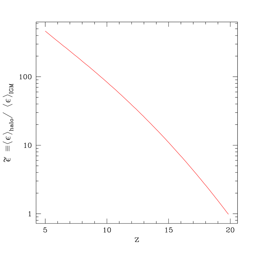
Figure 1: The relative halo/IGM free-free emissivity $\tilde{\epsilon}\equiv\langle\epsilon\rangle_{\rm halo}/\langle\epsilon\rangle_{\rm IGM}$ as a function of redshift, assuming that the entire uniform IGM is ionized. The contribution of halos to the comoving free-free emissivity dominates that of the IGM at all redshifts below 20.

where $L_{\nu}(M,z)$ is given by equations (4) and (5). The comoving free-free emissivity of the IGM may be estimated directly from equation (3), assuming the entire IGM is ionized. For the purpose of this calculation, we have assumed a uniform IGM and ignored the contribution of overdense structures without an internal source of ionizing radiation. This is a good approximation as the low ambient radiation field in the early universe means that these objects become self-shielding at low column densities and are the last objects to become reionized (Miralda-Escude, Haehnelt, & Rees, 1998). In Figure (1) we display the relative halo-IGM emissivity $\tilde{\epsilon}\equiv\langle\epsilon\rangle_{\rm halo}/\langle\epsilon\rangle_{\rm IGM}=\langle n_{e}^{2}\rangle_{\rm halo}/\langle n_{e}^{2}\rangle_{\rm IGM}$. For $z<20$, the halo emissivity dominates over the IGM emissivity (at high redshift, we underestimate $\tilde{\epsilon}$ as the IGM is only partially reionized. As computed by Haiman & Loeb (1998), full reionization in this model only occurs at $z\sim 13$). Note that this ratio also applies directly to recombination line emission. We conclude that the free-free and recombination line emission is dominated by discrete sources rather than a diffuse background.

3 Recombination line emission

3.1 H$\alpha$ emission

The H$\alpha$ flux density from an ionized halo as detected with a R=1000 filter may be estimated as:

$$J_{\rm H\alpha}=\frac{L_{H\alpha}}{4\pi d_{L}^{2}}\frac{1}{\Delta\nu}\approx 625\left(\frac{1+z}{10}\right)^{-1}\left(\frac{R}{1000}\right)\left(\frac{\rm M}{10^{9}{\rm M_{\odot}}}\right){\rm nJy}$$ (10)

where we have estimated $L_{H\alpha}$ from equations (2) and (5). Note that the line width of H$\alpha$ is simply given by Doppler broadening $\Delta\lambda/\lambda\sim 10^{-4}(b/30{\rm kms^{-1}})$ (unlike the Ly$\alpha$ line, which will have broad damping wings), so it is still not resolved at R=1000. Using a narrow bandpass enables us to reduce the amount of background noise. Let us compare with the prospects for observability in the infra-red, which corresponds to rest-frame UV emission. The UV continuum emission in the rest frame 1500–2800 Å(longward of the Lyman limit) for a Salpeter IMF is $L_{\nu}=8\times 10^{27}\left(\frac{{\rm SFR}}{\rm 1M_{\odot}yr^{-1}}\right)=8\times 10^{27}\left(\frac{\rm\dot{N}_{ion}}{\rm 10^{53}photons\,s^{-1}}\right){\rm erg\,s^{-1}Hz^{-1}}$ (Madau 1998). Using equation (5), this translates into an observed IR flux density:

$$J_{\rm IR}=\frac{L_{\nu}}{4\pi d_{L}^{2}}(1+z)\approx 16\left(\frac{1+z}{10}\right)^{-1}\left(\frac{\rm M}{10^{9}{\rm M_{\odot}}}\right){\rm nJy}$$ (11)

Hence, $J_{\rm H\alpha}/J_{\rm R}\approx 40(R/1000)$. Note that the spectral energy distribution/IMF of a luminous source can be probed by its color, while the ratio of the H$\alpha$ luminosity to the rest frame UV luminosity will constrain the escape fraction of ionizing photons.

Let us examine the competitiveness of H$\alpha$ with continuum IR imaging with NGST. The signal to noise ratio of an observation with exposure time $t$ is given by (Gillett & Mountain 1998):

$$\frac{\rm S}{\rm N}=\frac{I_{s}t}{(I_{s}t+I_{bg}t+n\cdot I_{dc}\cdot t+n\cdot N_{r}^{2})^{1/2}}$$ (12)

where $I_{s}=1.5\cdot 10^{7}A\cdot\epsilon\cdot 1/R\cdot j_{\nu}\cdot f$ electrons ${\rm s^{-1}}$ is the signal photocurrent ($A$ is the area of the primary mirror in $m^{2}$, $\epsilon$ is the detector quantum efficiency ($\epsilon>80\%$ for $\lambda<5\mu$m, $\epsilon>50\%$ for $\lambda>5\mu$m), $j_{\nu}$ is the source strength in Jy, and f is the fraction of source photons collected ($f\approx 0.7$ for $\lambda<3.5\mu$m and $f\approx 0.5$ for $\lambda>3.5\mu$m)), $I_{bg}=1.5\cdot 10^{7}A\cdot\epsilon\cdot 1/R\cdot\beta_{\nu}\cdot\Omega$ electrons ${\rm s^{-1}}$ is the background photocurrent ($\beta_{\nu}$ is the background in Jy ${\rm sr}^{-1}$), $n\approx 4$ is the number of pixels required to cover $\Omega\approx 0.01\,{\rm arcsec^{2}}$, $I_{dc}$ is the detector dark current, and $N_{r}<15\,e\,{\rm read^{-1}}$ (Stockman et al 1997) is the read noise per pixel. We assume a point source subtends $\Omega\approx{\rm max}(1,(\lambda/3.5\mu m))\,0.01\,{\rm arcsec^{2}}$. For $\lambda=0.5-5\mu$m, the projected dark current is $I_{dc}<0.02{\rm e\,s^{-1}}$ for a Si:As IBC array, while for $\lambda>5\mu$m with an InSb array, $I_{dc}<1{\rm e\,s^{-1}}$ (Stockman et al 1997). To estimate the sky background, we consider twice the sky background observed by COBE (Hauser et al 1998). The sky background is measured at $1.25,2.2,3.5,4.9,12,25,60\mu$m. We assume the full wavelength dependence of the sky background in our calculations, employing a spline interpolation between the observed points. Roughly speaking, the background is $<10^{-5}\ {\rm Jy\ arcsec}^{-2}$ in the range $\lambda\sim 1-5\mu$m, and rises to $\sim 5\times 10^{-4}\ {\rm Jy\ arcsec}^{-2}$ for $\lambda>10\,\mu$m. An additional source of noise is thermal emission from the primary mirror, which we approximate as a 75K blackbody (Barsony, 1999). This exceeds the sky background at $\lambda\sim 10\mu$m, and thus only affects sources in H$\alpha$ emission with $z>15$. For IR continuum imaging ($R=3$) at $\lambda\sim 1-5\mu$m, the sky background is the dominant source of noise. Thus, we have ${\rm S/N(IR)}\approx 0.5(\Omega/{\rm 0.01\,arcsec^{2}})^{-1/2}\left(\frac{1+z}{10}\right)^{-1}\left(\frac{\rm M}{10^{9}{\rm M_{\odot}}}\right)t^{1/2}$. So, for instance, a 10$\sigma$ detection of our canonical $10^{9}M_{\odot}$ source at z=9 would take 400s. For spectroscopic applications with $R>1000$, the detector noise is the dominant source of noise. The increase in dark current at $\lambda>5\mu$m corresponds to reduced a signal to noise ratio for sources with $z>6.6$, leading to ${\rm S/N(H\alpha;z<6.6,z>6.6)}\approx(0.7,0.06)\,(\Omega/{\rm 0.01\,arcsec^{2}})^{-1/2}\left(\frac{1+z}{10}\right)^{-1}\left(\frac{\rm M}{10^{9}{\rm M_{\odot}}}\right)t^{1/2}$. A 10$\sigma$ detection of our canonical $10^{9}M_{\odot}$ source at z=9 in H$\alpha$ would take $3\times 10^{4}$s. Note that since the flux density $j_{\nu}^{H\alpha}\propto R$, the signal to noise is independent of the spectral resolution $R$ in the dark current limited regime $R>1000$. Thus, even higher resolution spectroscopy, up to the point when the $H\alpha$ line is resolved ($R\sim 10^{4}$), should be possible. We derive the useful rule of thumb that:

$$\frac{\frac{\rm S}{\rm N}({\rm H}\alpha)}{\frac{\rm S}{\rm N}({\rm IR})}(z<6.6,z>6.6)=(1.4,0.12)\left(\frac{t_{{\rm H}\alpha}}{t_{\rm IR}}\right)^{1/2}$$ (13)

Thus, for sources which sit at $z<$6.6, a source may be detected in IR imaging and H$\alpha$ spectroscopy in equal amounts of time. For sources at z$>$6.6, when the detector dark current for H$\alpha$ detection is signficantly larger, detection in H$\alpha$ requires an integration time 100 times longer than in IR imaging to achieve the same signal to noise ratio. This ratio will be reduced if advances in technology permit smaller dark currents at $\lambda>5\mu$m.

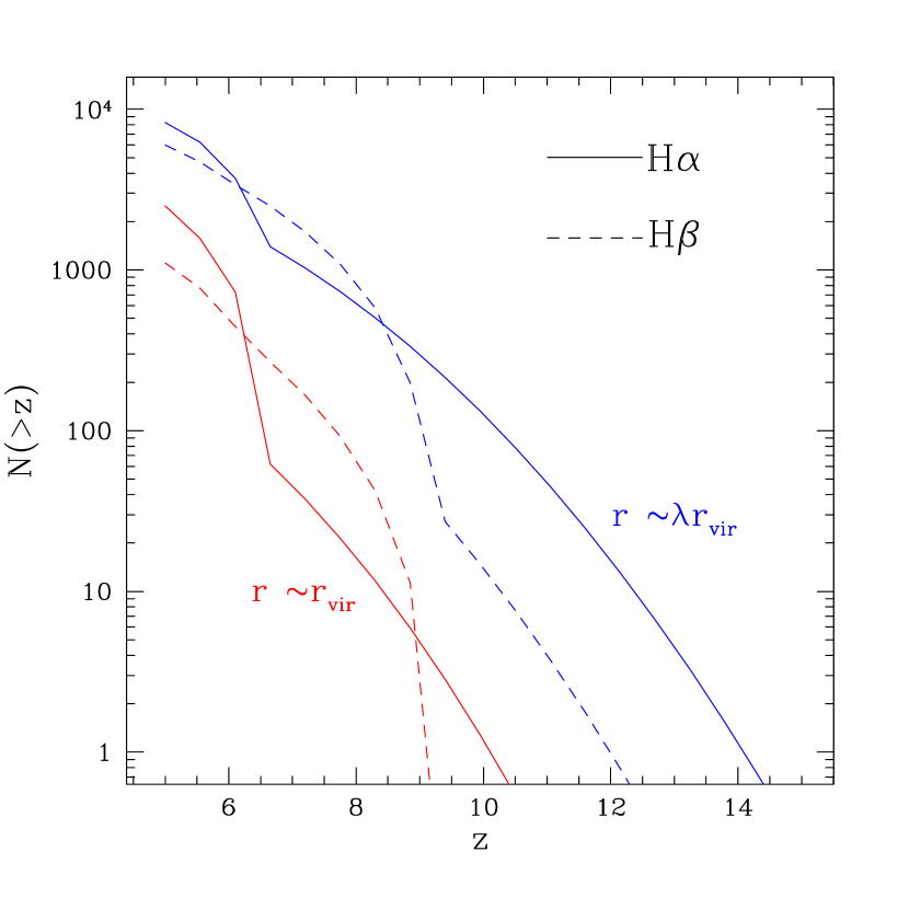
Figure 2: Number of sources in $4^{\prime}\times 4^{\prime}$ NGST field of field with a redshift greater than z, detectable with H$\alpha$, H$\beta$ spectroscopy (solid and dashed lines respectively) as a 10$\sigma$ fluctuation with $t=10^{4}$s, and R=1000, for emission from a disc ($r\sim\lambda r_{vir}$, essentially a point source), and an extended source ($r\sim r_{vir}$). The dip at z=7,9 for H$\alpha$, H$\beta$ is due to increased detector noise at longer wavelengths $\lambda>5\,\mu$m. Note therefore the existence of an interval where H$\beta$ is potentially easier to detect than H$\alpha$.

Note that the detection rate depends on the angular extent of the sources, even in the dark current limited regime. An extended source covers more pixels, resulting in a higher dark current (in very extended sources, it may be best to focus on the central pixels, which contain most of the light). For this reason, we quote the relative signal to noise in equation (13), which is independent of the angular size. In figure (2), we show the number of sources detectable with a S/N of 10 with $R>1000$ spectroscopy in $10^{4}$s ($\sim 3$ hours) of integration time, all computed using the full expression (12), for both disk-like ($r\sim\lambda r$) and extended ($r\sim r_{vir}$) objects. At least several thousand objects with $z>5$ may potentially be detected in the NGST $4^{\prime}\times 4^{\prime}$ field of view. The actual detection rate, of course, depends on the targeting strategy for spectroscopy (see discussion below). Note that if the star formation efficiency is lower, then the detection rate falls. In figure (7), we show the detection rate for $f_{star}\sim 1.7\%$, rather than $f_{star}\sim 17\%$. For a star formation efficiency lower by an order of magnitude, an integration time 100 times longer is required to obtain the same number counts.

It should be possible to observe higher order Balmer lines as well. For case B recombination with $n_{e}=100\,{\rm cm^{-3}}$ (the density dependence is fairly weak), $f_{\rm H\beta}/f_{\rm H\alpha}=0.35$ (Osterbrock 1989). Accounting also for the different $\delta\nu=\nu/R$ for H$\alpha$ and H$\beta$, we find that $S/N({\rm H\beta})/S/N({\rm H\alpha})=0.25$ for a given source, which implies an integration time 16 times longer is required to observe a source in H$\beta$ with the same signal to noise ratio as in H$\alpha$ (note that we assume that attenuation effects are still unimportant for H$\beta$, which is of shorter wavelength than H$\alpha$ and thus more suspectible to dust extinction or stellar absorption). However, in the redshift range $6.6<z<9.5$, the H$\beta$ line falls in the regime $\lambda<5\mu$m with low dark current, while the H$\alpha$ line falls in the $\lambda>5\mu$m regime with high dark current. In this case $S/N({\rm H\beta})/S/N({\rm H\alpha})=2$, i.e., the H$\beta$ line is potentially easier to observe than the H$\alpha$ line. Observing the H$\beta$ line should provide a firmer redshift identification, while the H$\alpha$/H$\beta$ ratio gives a useful measure of extinction. In figure (2), we show the detection rate of the H$\beta$ line as a function of redshift.

How can we pick out potential high redshift targets for spectroscopy? They may be quickly identified via continuum imaging using the Lyman-break technique successfully used at low redshifts (Steidel et al 1996). Beyond the redshift of reionization, an analogous technique using the Gunn-Peterson trough to detect dropouts can be used. Photometric redshifts may be supplemented by a narrow band filter search ($R\sim 100-400$) to isolate $H\alpha$ bright galaxies in a narrow redshift range. The filter width involves some trade-offs: the filter should be broad enough to cover a sufficiently large comoving volume, yet narrow enough that the flux density in H$\alpha$ greatly exceeds continuum flux densities. Note that current plans for NGST allow for multi-object spectroscopy in the NIR $1-5\mu$m range, using micro-mirrors but only single slit spectroscopy in the MIR range, $5-20\mu$m (Stockman et al 1997). However, even in the NIR a grating spectrograph will be able to perform spectroscopy for only a few hundred ($\sim$ several percent) of the objects in the field of view at a given time, thus requiring many pointings to complete a survey. Alternatively, a promising proposal is the Infrared Fourier Transform Spectrograph (IFTS) (Graham et al 1998) which will be able to perform panchromatic observations in the $1-15\mu$m range (which is the desired $z<20$ range for H$\alpha$ observations). It will be able to acquire both broad band imaging data and higher spectral resolution data (R=1-10000) for all objects in the field of view simultaneously, with very high (near $100\%$) throughput. Thus, the need for object preselection is obviated, and such an instrument would be extremely well suited for our purposes.

3.2 Comparison with Ly$\alpha$

While ionizing objects are expected to be more luminous in Ly$\alpha$ than in H$\alpha$, detection in H$\alpha$ has a number of nice features. Firstly, since H$\alpha$ is emitted in rest-frame optical, it is less susceptible to attenuation by dust than Ly$\alpha$, or rest-frame UV continuum. It is thus a significantly cleaner tracer of the star formation rate. Furthermore, the resonant scattering of Ly$\alpha$ photons within the HII region and in surrounding HI regions means that they will diffuse over a large region, resulting in an unobservably low surface brightness. The large optical path of Ly$\alpha$ photons as they random walk out of these regions greatly increases their probability of absorption by dust (Charlot & Fall 1993). Finally, the observability of Ly$\alpha$ is affected by complex velocity flows of the neutral gas, which may be outflowing from the ionizing source (thus, for instance, the observation of P-Cygni type profiles in local star-forming galaxies (see Kunth el al 1998 and references therein)). Note that 50% of the objects selected by the Lyman-break technique show no emission in Ly$\alpha$, while the rest have weak rest-frame equivalent widths $<20\,{\rm\AA}$ (Steidel et al 1996). By comparison, the expected rest-frame equivalent widths of star-forming galaxies from modelling their spectral energy distribution is ${\rm W_{\alpha}}\sim 100-200\,{\rm\AA}$ (Charlot & Fall 1993). Also, note that quasars are expected to have equivalent widths in the quasar rest frame of ${\rm W_{\alpha}}=0.68\frac{c}{\nu_{\alpha}f_{c}}\int^{\infty}_{\nu_{L}}d\nu f_{\nu}/\nu\approx 827\alpha^{-1}(3/4)^{\alpha}{\rm\AA}=360{\rm\AA}(\alpha=1.5)$ (Charlot & Fall 1993), where $\nu_{L},\nu_{\alpha}$ are the Lyman limit and Ly$\alpha$ frequencies, $f_{c}$ is the continuum flux near Ly$\alpha$, and $f_{\nu}\propto\nu^{-\alpha}$ blueward of Ly$\alpha$. In fact, most bright quasars are observed to have rest-frame equivalent widths of $50\leq{\rm W_{\alpha}}\leq 150{\rm\AA}$ (Schneider, Schmidt & Gunn 1991, Baldwin, Wampler & Gaskell 1989). This could be due to covering of the AGN source by HI clouds or dust extinction effects. We tentatively conclude that even in the post-reionization epoch, a Ly$\alpha$ survey is an inefficient means to search for ionizing sources. Until recently, H$\alpha$ surveys of high-z objects have not been carried out due to the difficulties of infrared spectroscopy from the ground. It is intriguing to note that recent such H$\alpha$ surveys (Glazebrook et al 1998) show a star formation rate approximately three times as high as that inferred from the 2800 ${\rm\AA}$ continuum luminosity by Madau et al (1996). This reinforces the expectation that surveys in UV continuum and Ly$\alpha$ tend to underestimate the star formation rates as they are subject to highly uncertain dust extinction effects.

Most importantly for our purposes, a H$\alpha$ survey would be able to detect ionizing sources prior to the epoch when HII regions overlap, when the universe was optically thick to Ly$\alpha$ photons. In order for Ly$\alpha$ emission from a source to be unaffected by resonant scattering, the ionizing source must ionize a region large enough for the Ly$\alpha$ photon to redshift out of the Gunn-Peterson damping wing. This problem has been considered by Miralda-Escude (1998). Given that the optical depth of the Gunn-Peterson damping wing as a function of displacement $\Delta\lambda$ from line center, $\tau(\Delta\lambda)=1.7\times 10^{-3}(1+z/10)^{3/2}(\Delta\lambda/\lambda)^{-1}$, a region $r\sim 1$ Mpc in proper size must be ionized, independent of redshift, in order to have $\tau(\Delta\lambda)\sim 0.3$. Note that this is somewhat greater than the proper radius of influence of a single ionizing source at z=9, $r_{\rm influence}\sim 0.1{\rm Mpc}(M/10^{9}M_{\odot})^{1/3}(1+z/10)^{-2}$ (assuming the source never reaches its equilibrium Stromgren radius). Nonetheless, the clustering of ionizing sources means that many should exist in large, overlapping ionized regions. Even if an ionized region $r\sim 1\,$Mpc is created, the high recombination rate due to the higher IGM densities are high redshift results in a residual neutral fraction which is optically thick to Ly$\alpha$. If we take the column density to be $N_{HI}\sim xn_{b}r$, where $x$ is the ionization fraction in ionization equilibrium, then the optical depth to Ly$\alpha$ scattering in transversing this region is:

$$\tau_{o}\simeq 100\left(\frac{1+z}{10}\right)^{6}(1+\delta_{b})^{2}\left(\frac{J_{21}}{0.5}\right)\left(\frac{T}{10^{4}K}\right)^{-0.7}$$ (14)

where $J_{21}$ is the background ionizing intensity in units of $10^{-21}{\rm erg\,s^{-1}\,cm^{-2}\,Hz^{-1}\,sr^{-1}}$, and $\delta_{b}=\delta\rho_{b}/\rho_{b}$ is the gas overdensity. It therefore seems dubious that unscattered Ly$\alpha$ can be observed except in highly underdense regions, or unless ionizing sources are considerably more luminous than we have considered.

Loeb & Rybicki (1999) have considered the observational signature of Ly$\alpha$ emission of an ionizing halo, given that the Ly$\alpha$ photons are likely to resonantly scatter in the surrounding neutral IGM, before redshifting out of resonance. They find that the Ly$\alpha$ photons emitted by a typical source at $z\sim 10$ scatter over a characteristic angular radius of $\sim 15^{\prime\prime}$ around the source and compose a line which is broadened and redshifted by $\sim 10^{3}{\rm km\,s^{-1}}$. However, the large angular scale leads to a very low surface brightness. Adopting the same estimates as the previous section for instrumental noise and the IR background, we find that the signal is likely to be overwhelmed by instrumental noise. Assuming $\dot{N}_{\rm Ly\alpha}\approx\dot{N}_{ion}$, so that the flux $f_{\rm Ly\alpha}\approx 12f_{\rm H\alpha}$ and the flux density $j_{\rm Ly\alpha}\approx 2.2j_{\rm H\alpha}$ (Case B), the relative signal to noise ratio at the same spectral resolution is given by:

$$\frac{\frac{\rm S}{\rm N}({\rm Ly}\alpha)}{\frac{\rm S}{\rm N}({\rm H\alpha})}(z<6.6,z>6.6)=(8\times 10^{-3},0.1)\left(\frac{\Omega_{\rm H_{\alpha}}}{0.01{\rm arcsec^{2}}}\right)^{1/2}\left(\frac{\Omega_{\rm Ly_{\alpha}}}{700{\rm arcsec^{2}}}\right)^{-1/2}$$ (15)

(in fact, line broadening for Ly$\alpha$ is likely to further lower this ratio by a factor of a few). Thus, with ${\rm S/N(Ly\alpha)}=6\times 10^{-3}(\Omega/700{\rm arcsec^{2}})^{-1/2}\left(\frac{1+z}{10}\right)^{-1}\left(\frac{\rm M}{10^{9}{\rm M_{\odot}}}\right)t^{1/2}$, our canonical source $10^{9}{\rm M_{\odot}}$ source at z=9 would require an unacceptably long integration time of 32 days for a 10$\sigma$ detection. If even trace amounts of dust are present, the large number of resonant scatterings means that the Ly$\alpha$ signal is likely to be severely attenuated. We conclude that this would be a very difficult observation, although extremely interesting if carried out successfully. In particular, it would be very interesting to view the same bright source in Ly$\alpha$ and H$\alpha$. Their relative intensities would establish the importance of dust extinction, while their relative spatial extent would constrain the topology of neutral gas surrounding the source. Note that Loeb & Rybicki (1999) assume a uniform IGM surrounding the source. If the surrounding IGM is inhomogeneous, the Ly$\alpha$ photons are likely to diffuse along the underdense directions, leading to a signal of even lower surface brightness. In addition, Lyman limit systems will absorb a certain fraction of the Ly$\alpha$ photons (since photons scattering in these systems are no longer redshifting out of resonance).

4 Free-free emission

Free-free emission from galaxies forms a fluctuating background in radio frequencies similar to the EBL sought in the optical (Vogeley 1997) and the CIB sought after in the infra-red (Kashlinsky et al 1996, Dwek et al 1998). It is has the potential to yield a great deal of useful information in that it is a direct tracer of star formation and clumping, it is unaffected by dust, there are no unknown K-corrections to be applied (due to the flat spectrum nature of free-free emission), and sources at very high redshifts (z $>$ 10) make a significant contribution and are still potentially observable. We adopt two approaches in characterizing the Free-Free Background (FFB): detecting the mean signal (via spectral distortion of the CMB) and detecting the fluctuating signal (by direct imaging of ionized halos or detecting temperature fluctuations across the sky).

4.1 Spectral distortion

Consider first the mean sky averaged signal $\langle S\rangle$. The integrated emission from ionized halos creates a spectral distortion of the CMB which is potentially observable. Note that for a given mean surface brightness $\langle S\rangle$, the temperature perturbation rises quadratically at low frequencies, where (in the Rayleigh-Jeans limit) $\Delta T_{ff}=c^{2}\langle S\rangle/2k\nu^{2}$. This spectral distortion may be characterised by the optical depth to free-free emission (Bartlett & Stebbins 1991) $Y_{ff}=\frac{\Delta T_{ff}}{T_{\gamma}}x^{2}$ where $T_{\gamma}$ is the undistorted CMB photon temperature, $x\equiv h\nu/kT_{\gamma}$ and $\Delta T_{ff}=T_{\rm eff}-T_{\gamma}$ is the mean temperature perturbation created by free-free emission (note that the $Y_{ff}$ has a different spectral form from Compton y-distortion (parameterized by $y$), arising from Compton scattering of CMB photons off hot gas). The quadratic nature of the distortion means that a bound on $Y_{ff}$ is best obtained by comparing temperature measurements at high frequencies (when the perturbation due to free-free emission is small) and low frequencies (when it becomes important). The CMB blackbody temperature near the peak of emission has been measured by the FIRAS instrument aboard COBE to be $T_{\gamma}=2.768\pm 0.004$K (95% CL) (Fixsen et al 1996), while at low frequencies the effective temperature has been measured as $T_{\rm eff}=2.65^{+0.33}_{-0.30}$K at 1.4 GHz (Staggs et al 1996a) and $T_{\rm eff}=2.730\pm 0.014$K at 10.7 GHz (Staggs et al 1996b). Combining the limits on extant data to compute $\Delta T_{ff}$, one obtains $Y_{ff}<1.9\times 10^{-5}$ (95% CL) (Smoot & Scott 1996). Significant amounts of free-free emission can still be present without violating this constraint. At low frequencies, it corresponds to a limit on the mean temperature perturbation:

$$\Delta T_{ff}\leq 4.4\times 10^{-2}\left(\frac{\nu}{2GHz}\right)^{-2}\ K$$ (16)

One of the chief goals of the DIMES satellite (Kogut 1996) is to measure spectral distortions from free-free emission at low frequencies. DIMES will have a frequency coverage 2–100 GHz and a sensitivity $0.1$mK (at 2 GHz). It is hoped that a measurement of $\Delta T_{ff}$ will indicate the optical depth of the ionized IGM and thus constrain the redshift of reionization $z_{r}$. However, we have already seen from quite general arguments in section 2.2 that the mean emission from ionized halos should dominate that of the IGM. One can examine this in more detail. The equation of cosmological radiative transfer (Peebles 1993) gives the observed surface brightness of the ionized IGM as:

$$J(\nu_{o})=\frac{1}{4\pi}\int_{0}^{z_{r}}dz\frac{dl}{dz}\frac{\epsilon(\nu(1+z))}{(1+z)^{3}}$$ (17)

where $\epsilon$ is given by equation (3). If $z_{r}=13$, as in our model, then this translates into $\Delta T_{ff}=c^{2}J/2k\nu^{2}=6\times 10^{-6}$K at 2GHz, which is beyond the 0.1mK sensitivity of DIMES, which will only be able to detect $z_{r}>85$ for the $\Lambda$CDM cosmology we have adopted. On the other hand, if we compute $\langle S\rangle$ from equation (8) (setting $z_{\rm min},S_{c}=0$ since point source removal is not possible with the $10^{\circ}$ beam of DIMES), we obtain $\Delta T_{ff}=3.4\times 10^{-3}$K, well within the capability of DIMES, while still satisfying the y-distortion constraint by an order of magnitude. Note that we have assumed that free-free emitters are the only radio-bright sources in the sky. The existence of radio-loud galaxies and AGNs(see section 4.3.3 for discussion) is likely to increase the spectral distortion due to radio sources.

Thus, it is likely that any spectral distortion detected by DIMES will not constrain the reionization of the IGM but rather the integrated free-free and other radio emission from galaxies, which provides a stronger signal by at least an order of magnitude.

4.2 Direct Detection of Ionized Halos

A natural way to determine if an observed spectral distortion is due to free-free emission from the first ionized halos or the IGM is to attempt to directly detect sources with a high angular resolution instrument.

4.2.1 Detection of point sources

The free-free flux from an ionized halo may be estimated as:

$$S_{\rm ff}=\frac{L_{\nu}^{\rm ff}}{4\pi d_{L}^{2}}(1+z)\approx 2.5\left(\frac{1+z}{10}\right)^{-1}\left(\frac{\rm M}{10^{9}{\rm M_{\odot}}}\right)\left(\frac{\rm T}{10^{4}\,{\rm K}}\right)^{-0.35}{\rm nJy}$$ (18)

where we have estimated $L_{\nu}^{\rm ff}$ from equations (4) and (5). Assuming a point source, and the 0.1” resolution of the Square Kilometer Array (SKA), this translates into a brightness temperature of:

$$T_{b}^{ff}=0.09{\rm K}\left(\frac{\nu}{2\,{\rm GHz}}\right)^{-2.1}\left(\frac{T}{10^{4}{\rm K}}\right)^{-0.35}\left(\frac{M}{10^{9}M_{\odot}}\right)\left(\frac{1+z}{10}\right)^{-1}\left(\frac{\theta}{0.1^{\prime\prime}}\right)^{-2}$$ (19)

On the other hand, the detector noise may be estimated as (Rohlfs & Wilson 1996):

$$S_{\rm instrum}=\frac{2kT_{\rm sys}}{A_{\rm eff}\sqrt{2t\Delta\nu}}=10\left(\frac{\Delta\nu}{1\,{\rm GHz}}\right)^{-1/2}\left(\frac{t}{10^{5}\,s}\right)^{-1/2}{\rm nJy}$$ (20)

where we have used $A_{\rm eff}/T_{\rm sys}=2\times 10^{8}{\rm cm^{2}/K}$ for the SKA (Braun et al 1998), and we assume a bandwidth $\Delta\nu\approx 0.5\nu$. Thus, in 10 days, a 5$\sigma$ detection of a 16 nJy source is possible. This is a tremendous leap in sensitivity; the deepest observations with the VLA at 8.4 GHz (Partridge et al, 1997) with approximately a week’s total integration time were able to identify point sources at the 7 $\mu$Jy level (the rms sensitivity was $1.5\mu$Jy), with a resolution of 6”.

For a given integration time, the sensitivity for detection of a given halo in free-free emission with the SKA is significantly less than that for H$\alpha$ detection (with $R>1000$) with NGST. The relative signal to noise is:

$$\frac{\frac{\rm S}{\rm N}({\rm free-free)}}{\frac{\rm S}{\rm N}({\rm H\alpha})}(z<7,z>7)=(1.1\times 10^{-3},1.3\times 10^{-2})\left(\frac{\Delta\nu}{1\,{\rm GHz}}\right)^{1/2}\left(\frac{t_{\rm ff}}{t_{\rm H\alpha}}\right)^{1/2}$$ (21)

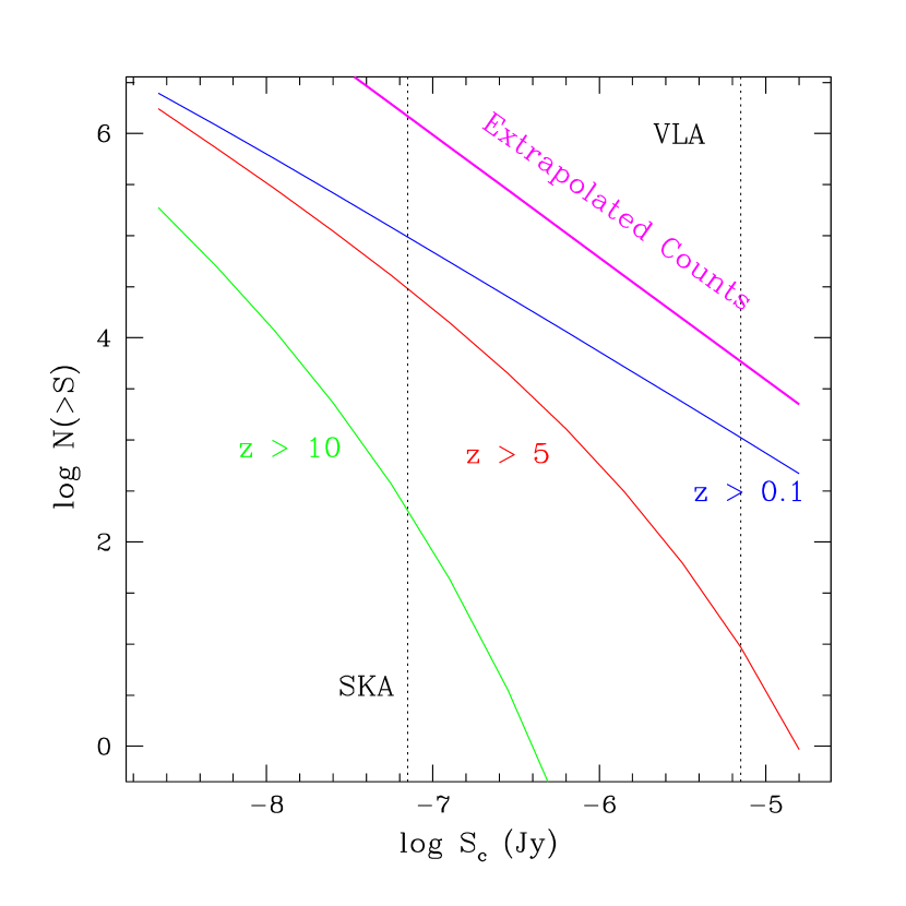
Figure 3: Number of sources which may be detected in the $1^{\circ}$ field of view of the Square Kilometer Array (the field of view for the VLA is similiar, $40^{\prime}\times 40^{\prime}$), as a function of the cut-off flux $S_{c}$. Realistic limiting fluxes for point source detection are shown. The extrapolated source counts from Partridge et al (1997) are also shown.

where the above ratio holds in the regime where free-free detection is limited by instrumental noise (for a discussion of confusion noise, see section (4.2.5)). Thus, the SKA will only be able to detect bright sources. However, note that its field of view is considerably larger than that of NGST–$1^{\circ}$ rather than 4’. In figure (3) we compute the number of sources detectable above a given flux threshold $S_{c}$. We find that $\sim 10^{4}$ sources with $z>5$ should be present in the 1 square degree field of view of the Square Kilometer Array above a source detection threshold of $70$nJy.

4.2.2 Power spectrum of unresolved sources

Identification of individual sources may not always be feasible. Many sources will too faint to be individually detected, or they may be crowded and blended together in a confused field. Such sources can still be detected statistically by observing the fluctuations in the FFB due to sources below the flux limit. The discreteness of sources create large amounts of small scale power. The power spectrum is white noise ($C_{l}\sim$ constant) until the angular scale of the beam (or the typical scale of a halo, if it is larger), beyond which it damps rapidly. We can compute compute the statistics of the background below the flux cut $S_{c}$, assuming the sources are unclustered. In particular, we compute the power spectrum of the fluctuations from equation (8):

$$C_{l}^{\rm Poisson}=\langle S^{2}\rangle=\int^{S_{c}}_{0}\frac{\partial N}{\partial S}S^{2}dS$$ (22)

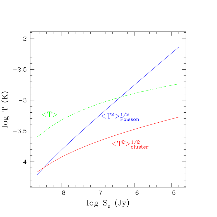
Figure 4: Mean and RMS temperature fluctuations for diffuse background below point source removal threshold $S_{c}$, at 2 GHz and 4” resolution. Note the steeper dependence of Poisson fluctuations on the flux cutoff $S_{c}$ compared to the clustering term.

(independent of $l$), and thus compute the rms temperature fluctuations from $T_{\rm rms}^{2}=\sum_{l}\frac{2l+1}{4\pi}C_{l}^{\rm Poisson}B_{l}^{2}\approx\frac{C_{l}^{\rm Poisson}}{4\pi\theta^{2}}$ where we have taken the beam of the telescope to be Gaussian: $B_{l}^{2}=e^{-l(l+1)\theta^{2}}$. Note that the rms temperature fluctuations increase with increasing resolution. In Figure (4) we display the computed rms temperature fluctuations at 2 GHz and with $4^{\prime\prime}$ resolution. Also shown is the mean signal $\bar{T}$, computed from the first moment of equation (8), which is independent of angular resolution. Our model is consistent with present observations. With $S_{c}=7\mu$Jy and $\theta=6^{\prime\prime}$ we obtain $\Delta T/T=9.5\times 10^{-5}$ at 8.4GHz, as compared with the measurement $\Delta T/T\approx 7\pm 8\times 10^{-5}$ of Partridge et al (1997), and within their 95% confidence limit $\Delta T/T<1.3\times 10^{-4}$.

Asssuming that galactic foregrounds are negligible (see section (4.2.5)), the main source of noise is instrumental. From equation (20), the rms sensitivity to temperature fluctuations for a beam of angular size $\theta$ is:

$$T_{noise}=0.35\,{\rm K}\left(\frac{\nu}{2\,{\rm GHz}}\right)^{-2.1}\left(\frac{\theta}{0.1^{\prime\prime}}\right)^{-2}\left(\frac{\Delta\nu}{1\,{\rm GHz}}\right)^{-1/2}\left(\frac{t}{10^{5}\,s}\right)^{-1/2}$$ (23)

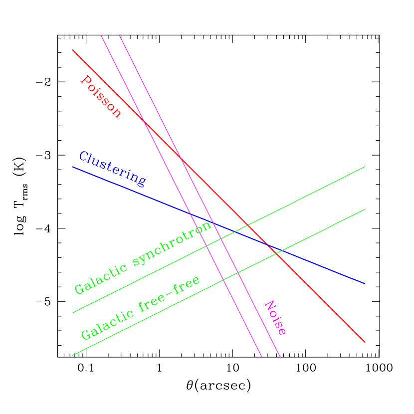
Figure 6: Angular dependence of $T_{rms}\equiv[\frac{l(l+1)C_{l}}{4\pi}]^{1/2}$ at 2 GHz, as a function of the beam FWHM $\theta$. Here the FFB is composed of sources with $S<S_{c}=70$nJy. Temperature fluctuations of the FFB increase with higher angular resolution, whereas the foregrounds damp rapidly. Also shown is the instrumental noise for integration times of 1 and 10 days. There exists a window in the $2^{\prime\prime}-20^{\prime\prime}$ range where the signal is greater than both instrumental noise and foregrounds. Note that the Poisson term is greater than the clustering term in this domain.

For the same parameters, and assuming a cut-off flux of $S_{c}=70$nJy, our expected signal is only $0.02$K. However, note that our expected signal $T_{rms}\propto\theta^{-1}$, whereas the instrumental noise $T_{\rm instrum}\propto\theta^{-2}$. By varying the size of the interferometer, we can vary the angular size of the beam, optimising it for this observation. Referring to figure (6), we see that on angular scales $\sim 1^{\prime\prime}-10^{\prime\prime}$, the temperature fluctuations due to the free-free background exceeds both the instrumental noise level and the galactic synchrotron foreground. Therefore, observing a radio field at coarser resolution increases the signal to noise ratio of temperature fluctuations sufficiently to enable the fluctuating free-free background to be detected. Note that if we simply smooth the map, the $T_{\rm instrum}\propto\theta^{-2}$ scaling is not strictly applicable. Smoothing the map corresponds to downweighting longer baseline information, which essentially means that some information is thrown away. This decreases the effective area and increases the detector noise, so $T_{\rm instrum}$ declines more gradually with $\theta$ (although still faster than $T_{rms}\propto\theta^{-1}$). The best solution would be to observe in a more compact configuration with resolution $\sim 1^{\prime\prime}-10^{\prime\prime}$ to begin with, so no data is thrown away. One wants to reach a compromise between the need for the high angular resolution required to beat down source confusion in discrete source identification and removal, and the somewhat lower angular resolution optimal for analysing the fluctuating residual signal, or confusion noise itself. A natural solution would be to work at an angular resolution $\theta_{\rm equal}$ where instrumental and confusion noise are comparable. Working at higher resolutions than this does not yield significant advantages for discrete source extraction, since the instrumental noise background in flux units is independent of angular resolution. By fiat, after source removal the instrumental noise and fluctuating signal are now about equal, and smoothing the fluctuating signal increases the signal to noise ratio sufficiently for an analysis to be undertaken. Note that source removal need not always be in the instrument noise dominated regime, $S_{c}=n_{\sigma}S_{\rm instrum}$. Source identification in a crowded field can be difficult, and not all sources can be removed down to the flux limit. If the angular size of typical objects is large, $\theta_{\rm typ}>\theta_{\rm equal}$, then confusion noise exceeds instrumental noise and $S_{c}>n_{\sigma}S_{\rm instrum}$. In this case, increasing the angular resolution beyond $\theta_{\rm typ}$ yields no advantage. Both because of the higher cut-off flux $S_{c}$, as well as the lower angular resolution, detecting the fluctuating signal will not be a problem. Furthermore, as we discuss in section (4.2.5), our model probably underestimates the temperature fluctuations which will be observed, which is likely to have components from other radio souces in the sky such as low-redshift radio galaxies and radio-loud AGNs.

The free-free component may be separated from other contaminants in multi-frequency observations by its spectral signature (flat spectrum, as opposed (for instance) to the $B_{\nu}\propto\nu^{-0.9}$ spectrum of synchrotron radiation). In addition, besides merely computing RMS temperature fluctuations, it would be desirable to compute the angular power spectrum of the observed signal and confirm its white noise character. In performing this analysis one has to take care to ensure that there is no aliasing of power on scales larger than the field of view (due to Galactic foregrounds and the CMB). This can be done by high-pass filtering and edge tapering the map. Besides the various sources of noise depicted in figure (6), one also has to contend with sample variance, given by:

$$(\Delta C_{l})^{2}=\frac{1}{f_{\rm sky}}\frac{2}{2l+1}C_{l}^{2}$$ (24)

where $f_{\rm sky}$ is the fraction of sky covered (this expression assumes the $C_{l}$’s are Gaussian distributed, as they should be by the Central Limit Theorem, since a large number of modes contribute). In addition, one probably will bin the computed $C_{l}$’s in bins of size $\Delta l$ to increase the signal to noise. Using $l\,\theta\sim\pi$, an angular resolution of $\theta\sim 4^{\prime\prime}$ corresponds to $l\sim 10^{5}$. The signal to noise for the sample variance term is $\frac{C_{l}}{\Delta C_{l}}=20\left(\frac{l}{10^{5}}\right)^{1/2}\left(\frac{\Omega}{1^{\circ}\,\Box}\right)^{1/2}\left(\frac{\Delta l}{100}\right)^{1/2}$, which may be increased by increasing the bin size $\Delta l$. Thus, sample variance should not pose any problems.

4.2.3 Clustering of ionized sources

Does clustering of the ionized halos make a significant contribution to fluctuations in the FFB? We find that on arcsecond scales and with a cutoff flux $S_{c}=70$nJy, Poisson fluctuations are more important than the contribution due to clustering. However, with a lower cutoff flux $S_{c}$, or on somewhat larger angular scales, the clustering term dominates.

First, let us consider the evolution of the halo correlation function with redshift. The matter correlation function may be computed as:

$$\xi_{mm}(r,z)=\int_{0}^{\infty}\frac{dk}{k}4\pi k^{3}P(k,z)\frac{sin\ kr}{kr}$$ (25)

However, halos which collapse early in the history of the universe consitute rare density peaks which are highly biased. In a linear bias model, the correlation function of halos is given by:

$$\xi_{hh}(M_{1},M_{2},r,z)=b(M_{1},z)b(M_{2},z)\xi_{mm}(r,z)$$ (26)

where the bias factor is given by Mo & White (1996):

$$b(M,z)=1+\frac{\nu^{2}-1}{\delta_{c}}=1+\frac{\delta_{c}}{\sigma^{2}(M,z)}-\frac{1}{\delta_{c}}$$ (27)

where $\delta_{c}=1.68$ and $\nu=\delta_{c}/\sigma(M,z)$. For simplicity we assume the correlation function of halos has the same shape at different redshifts, and differs only in amplitude. This assumption is shown to hold in numerical simulations (Kravtsov & Klypin 1998, Ma 1999), due to a cancellation of non-linear effects in the evolution of the power spectrum and bias factor. We assume $\xi_{mm}(r)$ is a power law on scales below the non-linear lengthscale (since this is shown to hold in numerical simulations), and is given by equation (25) on scales above the non-linear lengthscale. In Figure (5), we compute the halo correlation length $r_{o}^{halo}$ (defined as $\xi_{hh}(r_{o}^{halo},z)=1$) at each epoch $z$, assuming a number weighted bias factor

$$\tilde{b}(z)=\frac{\int_{M_{*}}^{\infty}b(M,z)n(M,z)dM}{\int_{M_{*}}^{\infty}n(M,z)dM}$$ (28)

The cutoff mass $M_{*}=10^{8}(1+z/10)^{-3/2}M_{\odot}$ introduces strong bias at high redshift, with the net result that the correlation length of halos decreases very slowly with redshift, despite the fall in the matter correlation length. For a higher cutoff mass, bias becomes important at lower redshift, and the initial dip seen in Figure (5) moves to lower redshift and is less pronounced. Thus, the observed clustering in the Lyman-break galaxy sample of Giavalisco et al (1998), with a comoving correlation length at $z\sim 3$ comparable to that in the local universe, is consistent with a detection of the most luminous and massive ($M\sim 8\times 10^{11}h^{-1}M_{\odot}$) galaxies at that redshift. The clustering of ionising sources at high redshift is therefore non-negligible, and a potentially important effect in contributing to free-free background fluctuations.

The angular correlation function of the free-free background below a flux cut-off $S_{c}$ is:

$$C(\theta,S_{c}) = \left(\frac{1}{4\pi}\right)^{2}\int_{0}^{\infty}dz\frac{dl}{dz}\frac{j_{eff}^{2}(z,S_{c})}{(1+z)^{6}}\int_{-\infty}^{\infty}d\Delta\xi_{hh}(r,z)$$

$$= \left(\frac{1}{4\pi}\right)^{2}\int_{0}^{\infty}dz\frac{dl}{dz}\left[\int_{S_{min}(z)}^{S_{c}}dS\frac{dN}{dVdS}\left(\frac{4\pi d_{L}^{2}S}{(1+z)}\right)b(S,z)\right]^{2}\ \int_{-\infty}^{\infty}d\Delta\xi_{mm}(r,z)$$

where $j_{eff}(S_{c},z)$ is the proper free-free emissivity of halos at redshift $z$ below the flux limit $S_{c}$, and $b(S,z)=b(M(S,z),z)$. We use the small angle approximation $r^{2}=\Delta^{2}+d_{A}^{2}\theta^{2}$, an excellent approximation since the clustering length covers a small part of the sky, $r_{o}/d_{A}\ll 1$. The contribution to the angular power spectrum due to clustering $C_{l}^{\rm cluster}$ is then straightforwardly computed from the Legendre transform of the correlation function:

$$C_{l}^{\rm cluster}=2\pi\int d(cos\theta)P_{l}(cos\theta)C(\theta)\approx 2\pi\int_{0}^{\infty}\theta d\theta J_{o}(l\theta)C(\theta)$$ (30)

where the last step is valid for $l\gg 1$.

In Figure (4), we show the dependence of the clustering term on the flux cutoff at fixed angular scale $\theta\sim 1^{\prime\prime}$. As we lower the flux cutoff $S_{c}$, the Poisson term declines more sharply than the clustering term, until the clustering term dominates. We can understand this intuitively: the Poisson term is dominated by rare bright objects just below the detection threshold. As we lower the detection threshold, such objects are excluded from the residual FFB, leaving a more uniform distribution of faint objects. By contrast, the clustering term, like the mean brightness term, is dominated by faint, low mass objects. In particular, the amplitude of the clustering term is determined by the bias of objects at the mass cut-off, $M_{c}=10^{8}(1+z/10)^{-3/2}\,M_{\odot}$, rather than the bias of the rarer (though more highly biased) high mass objects. Thus, subtraction of bright sources decreases the Poisson term much more effectively than the clustering term. In Figure (6), we compute the amplitude of the clustering contribution to temperature fluctuations as a function of angular scale at fixed flux cutoff $S_{c}=70$nJy. We find that on the arcsecond scales on which the surface brightness of free-free fluctations exceeds instrumental noise and Galactic foregrounds (see below), the Poisson term is more important than the clustering term. However, at a lower flux cutoff the clustering term would dominate on these scales. Note the different angular dependence of the two terms: $C_{l}^{Poisson}\sim$const, whereas $C_{l}^{clustering}\propto l^{\gamma-3}$, where $\xi_{hh}\propto r^{-\gamma}$. On large scales, the matter correlation function falls below a power law, and eventually $C_{l}^{cluster}\propto l^{n}$ (where the linear power spectrum $P(k)\propto k^{n}$). This downturn is unimportant on the scales plotted, though it becomes appreciable on larger scales. At such low fluctuation amplitudes, both galactic foregrounds and intrinsic CMB anistropies dominate over the free-free signal.

4.2.4 Skewness

Another signature of residual discrete sources is the skewness they induce in maps (Refregier, Spergel & Herbig 1998). We compute this as the third moment of equation (8), $I_{3}=\Omega_{pix}\int_{0}^{S_{c}}dS\frac{dn}{dS}S^{3}\,{\rm Jy^{3}}$. The instrumental noise is Gaussian distributed, and thus has vanishing skewness. The 1$\sigma$ measurement uncertainty on this vanishing skewness is $\sigma[\eta_{instrum}]=\sqrt{\frac{6}{N_{pix}}}\sigma_{instrum}^{3}$, where $\sigma_{instrum}$ is the rms noise per pixel. Thus, the signal to noise of a skewness measurement is $\frac{S}{N}=\left(\frac{N_{pix}}{6}\right)^{1/2}\left(\frac{I_{3}}{\sigma_{instrum}^{3}}\right)$. We assume $\sigma_{instrum}\sim 1\mu$Jy for the VLA, and $\sigma_{instrum}\sim 10$nJy for the SKA, and also that point sources may be detected and removed at $S_{c}=7\mu$Jy for the VLA and $S_{c}=70$nJy for the SKA. The number of pixels is given by $N_{pix}=(FOV/\theta_{pix})^{2}$, where FOV=40’ for the VLA and FOV=$1^{\circ}$ for the SKA. We assume pixel sizes of order $\sim 10^{\prime\prime}$ for the VLA and $\sim 1^{\prime\prime}$ for the SKA. From equation (8) we obtain:$I_{3}=(1\mu{\rm Jy})^{3}$ for the VLA and $I_{3}=(12{\rm nJy})^{3}$ per pixel for the SKA. This translates into $S/N\approx 5^{3}(\theta/10^{\prime\prime})(\sigma_{\rm instrum}/1\mu Jy)^{3}(S_{c}/7\,{\rm\mu Jy})^{(4-\beta)}$ for the VLA and $S/N\approx 13^{3}(\theta/1^{\prime\prime})(\sigma_{\rm instrum}/10\,{\rm nJy})^{3}(S_{c}/70{\rm nJy})^{(4-\beta)}$ for the SKA, where $\frac{dn}{dS}\propto S^{-\beta}$ in the neighbourhood of $S_{c}$. The skewness is thus a very efficient way of detecting the residual field, potentially much more powerful than attempting to use the second moment. It uses the fact that free-free sources can only contribute positive temperature fluctuations, whereas fluctuations due to instrumental noise are symmetric about zero. It is thus a fairly robust statistic. Depending on how accurately Gaussian the instrumental noise is, the same exercise can be carried out with kurtosis. Note that we have assumed that Galactic foregrounds have no skewness. Given that their second moment damps rapidly at small scales (see below), both the amplitude and variance of the third moment is likely to be small. It would be interesting to look at existing VLA maps for residual skewness.

4.2.5 Foreground contamination

A possible concern is foreground source contamination. Note that due to the finite thickness of the surface of last scattering, CMB fluctuations damp rapidly beyond $l\sim 10^{3}(\theta\sim 0.1^{\circ})$. Thus, intrinsic CMB fluctations from the surface of last scattering contribute negligibly on the scales probed here, $C_{l}^{CMB}\approx 0$. One can filter out the large scale power with a filter function $F_{l}=1-e^{l(l+1)\sigma_{filter}^{2}}$, where $\sigma_{filter}\sim 0.1^{\circ}$. At small scales, the Galactic foregrounds $C_{l}\propto B(\nu)l^{-3}$ should damp rapidly(Tegmark & Efstathiou 1996, Bersanelli et al 1996), although note that the empirical $l^{-3}$ power law fit has only been observed for $l<300$ (Wright 1998); we assume this behaviour may be extrapolated to smaller scales. Below, we briefly summarise the estimated contributions from various foregrounds.

Galactic Free-free emission This component is dangerous as its spectral signature is identical to our signal. However, the large scale component of the Galactic free-free emission can be removed by cross-correlation with H$\alpha$ maps. For instance, the WhaM survey (Reynolds et al 1995; see http://www.astro.wisc.edu/wham) will map the northern sky at $1^{\circ}$ resolution down to 0.01 Rayleighs (1 Rayleigh=$2.41\times 10^{-7}{\rm erg\,s^{-1}cm^{-2}sr^{-1}}$), or $T_{ff}=17\mu{\rm K}T_{4}^{-0.35}\left(\frac{\nu}{2{\rm GHz}}\right)^{-2.15}$. We assume $B(\nu)\propto\nu^{-0.15}$ and normalise to the DIRBE analysis of Kogut et al (1996), which obtained rms fluctuations of 7.1 $\mu K$ at 53 GHz (COBE’s finite beam of course causes an underestimate of the rms fluctuations, but because $C_{l}\propto l^{-3}$ this is a negligible effect). This yields:

$$C_{l}^{free-free}=4.2\times 10^{-4}\left(\frac{\nu}{2{\rm GHz}}\right)^{-4.3}l^{-3}\ K^{2}\ sr$$ (31)

which translates into $\delta T^{free-free}=2.3\times 10^{-6}\left(\frac{\theta}{0.1^{\prime\prime}}\right)^{0.5}\left(\frac{\nu}{2{\rm GHz}}\right)^{-2.15}$ K.

Galactic Synchrotron We assume $B(\nu)\propto\nu^{-0.9}$ and normalise to an rms fluctuation of 11 $\mu K$ at 31 GHz, the upper limit of Kogut et al (1996), as indicated by a cross-correlation between 408 MHz and 19 GHz emission (de Oliveira-Costa et al 1998). This yields:

$$C_{l}^{syn}=6.1\times 10^{-3}\left(\frac{\nu}{2{\rm GHz}}\right)^{-5.8}l^{-3}\ K^{2}\ sr$$ (32)

which yields $\delta T^{syn}=8.6\times 10^{-6}\left(\frac{\theta}{0.1^{\prime\prime}}\right)^{0.5}\left(\frac{\nu}{2{\rm GHz}}\right)^{-2.9}$ K. The synchrotron emission may be identified and eliminated by its distinct spectral signature.

Extragalactic Point Sources Extragalactic point sources are essentially the signal we are looking for. In this paper, we predict the number of sources in a field of view above a certain flux $S_{c}$ which may be directly detected, as well as attempt statistical characterizations of the fluctuating background signal due to faint undetected sources. Here we pause to note two facts. Firstly, there are many other sources in the radio sky (radio galaxies, AGNs, etc) than the free-free emitters we have attempted to characterize. Secondly, when detecting point sources, the fluctuating signal due to undetected sources is also a source of confusion noise.

How do the figures in our model compare with existing observations? The deep radio survey by Partridge et al (1997) obtain a maximum likelihood estimate of the integral source count as:

$$N(\geq S)=(17\pm 2)\left(\frac{S}{1\mu{\rm Jy}}\right)^{-1.2\pm 0.2}{\rm arcmin^{-2}}$$ (33)

Assuming that most sources have flat spectra $I_{\nu}\propto\nu^{\alpha}$, where $\alpha\sim 0$ in this frequency range, we see from figure (3) that our model yields fewer sources than the observed number counts at 7$\mu$Jy by a factor of a few. Our admittedly crude model is not meant to be accurate at low redshift and ignores many contributions to the radio sky. Our low source counts, together with the fact that we satisfy present y-distortion bounds by an order of magnitude, indicate that the model employed is very conservative and probably underestimates the observable signal. On the other hand, extrapolating the observed source counts to fainter flux levels clearly overestimates the signal, as the mean flux $\langle S\rangle$ diverges and violates the y-distortion constraint. Evidently the source counts must turn over at low flux levels (in our model, this occurs because of the low mass cutoff $M_{*}$). To be conservative, we underestimate the signal to noise ratio of projected observations. Thus, we employ our semi-analytic model to estimate the fluctuating background signal, whereas when estimating confusion noise in point source detectation, we use the extrapolated source counts.

Note that we are not completely powerless to distinguish against contaminants, such as low redshift AGNs. If star formation occurs in an extended fashion across galactic halos, we should be able to spatially resolve our target sources, whereas AGNs would only show up as point sources. In addition, by observing at several frequencies, the observed spectral index $\alpha$ (where $S_{\nu}\propto\nu^{-\alpha}$) can be used to diagnose the origin of radio emission. In particular, it can be used to distinguish between thermal and non-thermal emission. Finally, as a zeroth order cut, our target high redshift galaxies should be amongst the faintest objects in a sample, both because of increased cosmological dimming, and the fact that collapsed objects at high redshift are intrinsically less massive and luminous.

We now estimate the confusion noise. Using equation (33), we can place an upper bound on the noise from residual undetected sources from $\langle S^{2}\rangle=\int^{S_{c}}_{0}\frac{\partial N}{\partial S}S^{2}dS=25.5\,S^{0.8}\mu{\rm Jy^{2}}\,{\rm arcmin^{-2}}$, which yields the white noise power spectrum:

$$C_{l}^{PS}=2.4\times 10^{-15}\left(\frac{S_{c}}{70{\rm nJy}}\right)^{0.8}\left(\frac{\nu}{2\ {\rm GHz}}\right)^{-4+2\alpha}\ {\rm K^{2}\,sr}$$ (34)

This gives $\delta T^{PS}=0.09{\rm K}\left(\frac{\theta}{0.1^{\prime\prime}}\right)^{-1}\left(\frac{S_{c}}{70{\rm nJy}}\right)^{0.4}\left(\frac{\nu}{2{\rm GHz}}\right)^{-2+\alpha}$, by far the leading contribution to foreground contamination at these frequencies and angular scales. We can compare the relative contribution of instrumental and confusion noise by demanding that the source flux cutoff be $n_{\sigma}\sim 7$ times the rms noise. In this case, using equation (20), we obtain $\frac{S_{confusion}}{S_{instrum}}=1.\left(\frac{\theta}{0.4^{\prime\prime}}\right)\left(\frac{n_{\sigma}}{7}\right)^{0.8}\left(\frac{\Delta\nu}{1\,{\rm Ghz}}\right)^{0.5}\left(\frac{t}{10^{5}s}\right)^{0.5}\left(\frac{\nu}{2\,{\rm GHz}}\right)^{\alpha}$. In the confusion noise dominated regime, the appropriate cut-off flux may be determined by directly comparing the flux received from a source at the cut-off flux $S_{c}$ and the background flux below this cut-off:

$$\frac{S}{N}\approx\frac{S_{c}}{(\langle S^{2}\rangle|_{S_{c}}\theta^{2})^{1/2}}=6\left(\frac{S_{c}}{70\,{\rm nJy}}\right)^{0.6}\left(\frac{\theta}{0.4^{\prime\prime}}\right)^{-1}$$ (35)

Confusion noise thus becomes the leading source of noise in discrete source identification and extraction at low angular resolution or if sources are extended rather than point-like, i.e., $\theta={\rm max(\theta_{beam},\theta_{object})}>0.4^{\prime\prime}$.

Will source crowding be a problem? If we extrapolate the Partridge et al (1997) counts down to $70$ nJy, then there will be $\sim 400$ sources per square arcmin, or $\sim 9{\rm arcsec^{2}}$ per source. With a maximum resolution of 0.1”, source crowding of bright point sources such as disks or mini-quasars should not be a problem. Even if the sources are extended, the angular extent of typical high redshift $M_{*}$ objects is small, $\theta_{vir}\sim r_{vir}/d_{A}<1^{\prime\prime}$. However, it is important to note that nothing is known about the appearance of the radio sky below $1\mu$Jy. It is possible that a host of extended low redshift, low surface brightness objects may suddenly surface at these flux levels.

4.2.6 Lower Star Formation Efficiency Case

Let us consider the lower star formation efficiency case where only $1.7\%$, rather than $17\%$, of the gas mass in halos fragments to form stars. This corresponds to an IGM metallicity at z=3 of $Z\sim 10^{-3}\,Z_{\odot}$, rather than $Z\sim 10^{-2}\,Z_{\odot}$. The net effect of the lower value is that while the number of sources remain the same, each source is an order of magnitude fainter. Thus, to obtain the same number counts as previous plots, an integration time 100 times longer is required. Also, the brightness of the fluctuating background is reduced, and is equivalent to removing discrete sources an order of magnitude fainter. The net result is that point source detection is likely to be instrument noise limited rather than confusion noise limited. Thus, after discrete source removal, the fluctuating residual background will be significantly harder to detect. In figure (7), we show results for the lower star formation efficiency, assuming the same integration time and source removal threshold as before. Note from the plot of foregrounds that the fluctuating background signal is only marginally detectable. Besides the RMS signal, the skewness is also reduced, to $I_{3}=(0.5\mu{\rm Jy})^{3}$ for the VLA (down from $I_{3}=(1\mu{\rm Jy})^{3}$) and $I_{3}=(5.5{\rm nJy})^{3}$ for the SKA (down from $I_{3}=(12{\rm nJy})^{3}$). Skewness at this level is still detectable, with S/N=$2.5^{3}(\theta/10^{\prime\prime})(\sigma_{\rm instrum}/1\mu Jy)^{3}(S_{c}/7\,{\rm\mu Jy})^{(4-\beta)}$ (VLA) and S/N=$5^{3}(\theta/1^{\prime\prime})(\sigma_{\rm instrum}/10\,{\rm nJy})^{3}(S_{c}/70{\rm nJy})^{(4-\beta)}$ (SKA).

The situation in reality is likely lie between the two scenarios we have considered, and thus the actual number counts is probably bracketed by our calculations. The temperature fluctuations in the residual field are detectable if discrete source removal is confusion limited; otherwise, it seems likely that only the non-gaussian signature of the residual field will yield useful information.

5 Kinetic Sunyaev-Zeldovich effect

Sunyaev-Zeldovich effects arise from the scattering of CMB photons off moving electrons, which result in brightness fluctuations of the CMB. They are a very attractive means of detecting high redshift objects, in part because of the well-known fact that the surface brightness of SZ effects is independent of redshift. This is because the increased energy density $(1+z)^{4}$ of the CMB at high redshift keeps pace with surface brightness dimming effects. Thus, since the angular size of an object of fixed physical size increases with redshift beyond $z\sim 2$, the SZ flux from a given object increases with redshift. The kinetic effect is given by $\frac{\Delta T}{T_{CMB}}=\frac{v}{c}\tau$ while the thermal effect is given by $(kT/m_{e}c^{2})\tau$, where the optical depth $\tau=\int n_{e}\sigma_{T}\,dr$. For the photoionized halos we are considering, typical temperatures are $T\sim 10^{4}$K. Their peculiar velocities are $v_{rms}\approx v_{o}D(z)^{1/2}\,{\rm km\,s^{-1}}$, where $D(z)$ is the growth factor (normalised to 1 today) and the characteristic one-dimensional velocity dispersion of galaxies in the local universe is $v_{o}\sim 600\,{\rm km\,s^{-1}}$ (Strauss & Willick 1995). Thus, $(v/c)/(kT/m_{e}c^{2})\sim 400(1+z/10)^{-1/2}$ and the kinetic effect dominates over the thermal effect. For an isothermal halo, we obtain $T^{SZ}_{b}\approx 3\times 10^{-7}\left(\frac{1+z}{10}\right)^{2}\left(\frac{M}{10^{9}M_{\odot}}\right)^{1/3}$ K, similar to the temperature fluctuation produced by a cluster in kinetic SZ at low redshift (the high redshift halo is $\sim 1000$ times smaller, but $\sim 1000$ times denser).

Unfortunately, this is likely to be difficult to detect. The flux from a halo is related to the temperature shift by:

$$S_{\nu}=\frac{2k^{3}T_{\gamma}^{2}}{h^{2}c^{2}}q(x)\int d\Omega|\Delta T_{\nu}(\theta)|=\frac{2k^{3}T_{\gamma}^{3}}{h^{2}c^{2}}q(x)\frac{v}{c}\sigma_{T}\frac{N_{e}}{d_{A}^{2}}$$ (36)

where $q(x)=x^{4}/4{\rm sinh}^{2}(x/2)$ is the spectral function, ,$x\equiv h\nu/kT_{\gamma}$, $T_{\gamma}=2.7{\rm K}$ is the CMB temperature, and $N_{e}=\int n_{e}d^{3}r\approx M/m_{p}(\Omega_{b}/\Omega_{m})$ is the total number of free electrons in the system. From the form of the spectral function, the kinetic SZ effect peaks at $\nu=217$ GHz. This is well beyond the frequency coverage of the SKA, which has an upper limit of 20 GHz. At this frequency, and taking $v\sim v_{rms}$, we obtain a flux density $S_{\nu}(20GHz)=0.24(\frac{M}{10^{9}M_{\odot}})(1+z/10)^{1.5}$nJy. Comparing with equation (18), the SZ flux density at 20 GHz is $\sim 10$ times less than the free-free flux density. We can maximise the SZ flux by going to higher frequencies. At the peak frequency, $S_{\nu}(217GHz)=9.6(\frac{M}{10^{9}M_{\odot}})(1+z/10)^{1.5}$nJy, and the kinetic SZ signal dominates over free-free emission. At these frequencies, the MMA (see http://www.mma.nrao.edu) would be the premier instrument, with a resolution of 0.1” at 230 GHz. However, its rms sensitivity at this frequency is 0.21 mJky/${\rm min}^{0.5}$, which means that even in a week’s integration time it will only be able to go down to $\mu$Jy levels. We conclude that SZ detection of high-redshift ionized halos is not possible in the near future.

However, it is worth noting that the SKA and MMA will be able to detect the kinetic SZ effect from the HII regions in the IGM blown by the first luminous sources. If the escape fraction is $f_{esc}\sim 20\%$ for our $10^{9}M_{\odot}$ source, it will be able to create an ionized region with $N_{e}\sim\dot{N}_{ion}t_{o}\sim 2\times 10^{67}$ electrons (using equation (5) and assuming the source lasts for $t_{o}\sim 10^{7}$yrs). This corresponds to a region $r_{comoving}=(3N_{e}/4\pi n_{comoving})^{1/3}\sim 1.2$ Mpc in size (note that $\dot{N}_{ion}/V_{\rm proper}\alpha_{B}n_{\rm proper}^{2}\sim 10^{-7}\ll 1$, so the effect of recombinations is negligible). Since this is much smaller than the coherence length of the velocity field, we assume all parts of the bubble are moving with a uniform peculiar velocity. From (36), we find that the flux from such an ionized bubble is $S_{\nu}(20{\rm GHz})=35$nJy (detectable by the SKA, which, using equation (20) and $A_{eff}/T_{sys}=1\times 10^{8}{\rm cm^{2}/K}$ at 20 GHz (Braun et al 1998) has a $S_{instrum}=6$nJy rms sensitivity) and $S_{\nu}(217GHz)=1.4\,\mu$Jy (detectable by the MMA). However, along any given line of sight one intersects not one but a multitude of ionized bubbles. Thus, the signal has to be detected statistically. Calculating the CMB fluctuations due to inhomogeneous reionization has been the subject of much recent work (Agahanim et al 1996, Grusinov & Hu 1998, Knox et al 1998; see also Haiman & Knox 1999, Natarajan & Sigurdsson 1999), and is beyond the scope of this paper. However, we make two observations. Firstly, predictions have focussed on the possibility of detection by Planck (detection by MAP seems unlikely). The temperature fluctuation power spectrum is generally white noise with a peak on the scale of a typical bubble; the induced $\Delta T/T\sim 10^{-6}-10^{-7}$. For the anistropies to be detectable by Planck, the bubbles need to have an unrealistically large size $r_{\rm comoving}\sim 10$Mpc. For bubbles with $r_{\rm comoving}\sim 1$Mpc, the anisotropies peak on sub-arcminute scales, beyond the angular resolution of Planck ($\theta_{\rm FWHM}\sim 5.5^{\prime}$ at 217 GHz; see http://astro.estec.esa.nl/Planck/). High resolution ground based instruments such as the SKA or MMA, which can easily resolve the bubbles, might be better suited to the task. Furthermore, the significantly larger collecting area of these instruments means that they will be more sensitive than Planck by about 3 orders of magnitude: with a year of observing time, the rms sensitivity of Planck at 217 GHz is at best $\sim 1$mJy. If we require that the sample variance be sufficiently low that $\delta\equiv C_{l}/\Delta C_{l}=10$, then using equation (24), we find that a map of size $\Omega=2(\delta/10)^{2}(l/10^{4})^{-1}(\Delta l/10^{2})^{-1}$ square degrees is sufficient. This is easily achievable with the SKA. Secondly, the signal due to inhomogeneous reionization (IR) is quite possibly smaller than that due to the Ostriker-Vishniac effect, which arises from the coupling between density and velocity fluctuations in a fully reionized medium (Haiman & Knox 1999, Jaffe & Kamionkowski 1998). To isolate the IR signal, it would be interesting to cross-correlate observed CMB fluctuations with the observed distribution of ionizing halos. They could either correlate positively (if halos blow ionized bubbles around themselves) or negatively (if underdense voids are reionized first).

6 Conclusions

In this paper, we have used a simple model based on Press-Schechter theory to make observational predictions for the detection of high redshift galaxies in free-free and H$\alpha$ emission. These signals are valuable as they directly trace the distribution of dense ionised gas at high redshift. Furthermore, they are relatively unaffected by dust or resonant scattering, and their intensities are directly related to one another. They can thus serve as a very powerful probe of the dark ages, and constitute promising applications of the new generation of instruments designed to probe this epoch, in particular the Next Generation Space Telescope (NGST) and the Square Kilometer Array (SKA).

A fairly robust prediction of our model is that the integrated free-free and other radio emission from ionizing sources will swamp the free-free emission from the ionized IGM by an least an order of magnitude. Thus, any spectral distortion of the CMB observed by DIMES at low frequencies will constrain the former quantity. This claim depends only upon the small escape fraction of ionizing photons from sources, as is observed in galaxies in the local universe. To evade it, the ionizing sources must themselves contain very little ionized gas, either because gas has been driven out by supernovae, or ionizing photons are able to escape through a hole in the ISM, leaving most of the gas in the host galaxy neutral.

The escape fraction of ionizing photons $f_{esc}$ from high redshift halos may be constrained by comparing the rest frame UV luminosities longward of the Lyman limit of the sources as observed by NGST, with the expected luminosities in H$\alpha$ and free-free emission. Given a model for the relative spectral energy distribution, the relative luminosities then directly constrain the escape fraction in halos at high redshift, an important quantity in theories on reionization. If this fraction is low, as we argue, then in a given amount of integration time, the H$\alpha$ emission from an ionized halo should be detected (with R=1000) with the same signal to noise as IR continuum imaging with NGST for $z<6.6$. For $z>6.6$, due to the increase in dark current noise in the $\lambda>5\mu$m regime, it will be detected with $10\%$ of signal to noise ratio of IR imaging. Higher order lines such as H$\beta$ should also be detectable. In addition, the SKA should be able to directly detect the same ionizing sources in free-free emission. While the NGST will be able to detect fainter sources than the SKA, the SKA has a larger field of view: $\sim$200 times larger in solid angle. We find that the SKA should be able to detect $\sim 10^{4}$ individual free-free emission sources with $z>5$ in its field of view. However, a large population of other radio bright sources (AGNs at low redshift, etc) will also be detected. NGST (which can obtain redshift information from the H$\alpha$ line) must therefore be used in conjunction with the SKA to distinguish between these two populations.

Free-free sources below the flux limit of the SKA constitute a fluctuating background which can be detected statistically. At arcsecond scales, Poisson fluctuations in the number of free-free sources create temperature fluctuations detectable by SKA. At such small scales, galactic foregrounds are expected to damp rapidly. We find that the expected clustering of high-redshift ionizing sources makes a negligible impact on the observed power spectrum of temperature fluctuations. These temperature fluctuations have a highly non-Gaussian signature. In particular, they should result in a detectable skewness. Finally, ionized gas at high redshift may also be detected by the kinetic Sunyaev-Zeldovich effect. While individual ionized halos are probably too faint to be detectable by the SKA or MMA, the ionized IGM around these halos create CMB anisotropies on sub-arcminute scales which should be detectable by these instruments.

I am grateful to my advisor, David Spergel, for his encouragement and guidance. I also thank Michael Strauss for many detailed and helpful comments on an earlier manuscript. Finally, I thank Nabila Aghanim, Gillian Knapp, Alexandre Refregier and Stephen Thorsett for helpful conversations. This work is supported by the NASA Theory program, grant number 120-6207.

Figure 5: Characteristic number weighted correlation length $r_{o}$ (comoving) as function of redshift, and corresponding angular scale $\theta_{o}\equiv r_{o}^{\rm proper}/d_{A}$. The bias of high redshift halos means that angular clustering does not plummet with redshift. For a higher cutoff mass $M_{*}$, bias becomes important at lower redshift. Beyond the turnoff, the angular scale of clustering is almost constant at a few arcminutes.

References

- (1)
- (2) Aghanim, N., Desert, F.X., Puget, J.L., & Gispert, R., 1996, A & A, 311, 1
- (3)
- (4) Baldwin, J.A., Wampler, E.J., & Gaskell, C.M., 1989, ApJ, 338, 630
- (5)
- (6) Barlett, J.G., & Stebbins, A., 1991, ApJ, 371, 8
- (7)
- (8) Barnes, J., & Efstahiou, G., 1987, ApJ, 319, 575
- (9)
- (10) Bersanelli, M., et al 1996, COBRAS/SAMBA: Report on the Phase A Study, ESA
- (11)
- (12) Barsony, M., 1999, private communication
- (13)
- (14) Bland-Hawthorn, J., & Maloney, P.R., 1999, ApJ, 510, L33
- (15)
- (16) Bond, J.R., Cole, S., Efstathiou, G., Kaiser, N., 1991, ApJ, 379, 440
- (17)
- (18) Braun, R., et al, 1998, Science with the Square Kilometer Array (draft), available at http://www.nfra.nl/skai/archive/science/science.pdf
- (19)
- (20) Burstein, D., Bender, R., Faber, S.M., & Nolthenius, R., 1997, AJ, 114, 1365
- (21)
- (22) Carroll, S.M., Press, W.H., Turner, E.L. 1992, ARA&A, 30, 499
- (23)
- (24) Charlot, S., & Fall, S.M., 1993, ApJ 415, 580
- (25)
- (26) Dalcanton, J.J., Spergel, D.N., Summers, F.J., 1997, ApJ, 482, 659
- (27)
- (28) Dekel, A. & Silk, J. 1986, ApJ, 303, 39
- (29)
- (30) Dwek, E., et al, 1998, ApJ, 508, 106
- (31)
- (32) de Oliveira-Costa, A., Tegmark, M., Page, L.A., Boughn, S.P., 1998, ApJ, 509, L9
- (33)
- (34) Dove, J.B., Shull, J.M., & Ferrara, A., 1999, ApJ, submitted, astro-ph/9903331
- (35)
- (36) Eisenstein, D., 1997, ApJ, submitted, preprint astro-ph/9709054
- (37)
- (38) Fixsen, D. J., Cheng, E. S., Gales, J. M., Mather, J. C., Shafer, R. A.,Wright, E. L., 1996, ApJ, 473, 576
- (39)
- (40) Giavalisco, M., Steidel, C.C., Adelberger, K.L., Dickinson, M.E., Pettini, M., Kellogg, M., 1998, ApJ, 503, 543
- (41)
- (42) Gillett, F.C., & Mountain, M., 1998, in Science with the NGST, ASP Conference Series Vol. 133, p. 42
- (43)
- (44) Glazebrook, K., Blake, C., Economou, F., Lilly, S., Colless, M., 1998, MNRAS, in press, astro-ph/9808276
- (45)
- (46) Grahams, J.R., Abrams, M., Bennett, C., Carr, J., Cook, K., Dey, A., Najita, J., Wishnow, E., 1998, PASP, 752, 1205
- (47)
- (48) Gruzinov, A., & Hu, W. 1998, ApJ, 508, 435
- (49)
- (50) Haiman, Z., & Loeb, A. 1997, ApJ, 483, 21
- (51)
- (52) Haiman, Z., & Loeb, A. 1998, ApJ, 503, 505
- (53)
- (54) Haiman, Z., & Knox, L. 1999, astro-ph/9902311, to appear in “Microwave Foregrounds” , eds. A. De Oliveira-Costa & M. Tegmark, ASP, San Francisco
- (55)
- (56) Hauser, M.G., et al 1998, ApJ, 508, 25
- (57)
- (58) Hummer, D.G., & Storey, P.J., 1987, MNRAS, 224, 801
- (59)
- (60) Jaffe, A., & Kamionkowski, M., 1998, Phys. Rev. D, 58, 043001
- (61)
- (62) Kashlinsky, A., Mather, J.C., Odenwald, S., & Hauser, M.G., 1996, ApJ, 470, 681
- (63)
- (64) Kennicutt, R., 1998, ApJ, 498, 541
- (65)
- (66) Knox, L., Scoccimarro, R., & Dodelson, S., 1998, Phys. Rev. Lett., 81, 2004
- (67)
- (68) Kogut, A., 1996, astro-ph/9607100
- (69)
- (70) Kogut, A., et al 1996 ApJ, 464, L5
- (71)
- (72) Kravtsov, A., & Klypin, A., 1998, ApJ, submitted, astro-ph/9812311
- (73)
- (74) Kunth, D., Terlevich, E., Terlevich, R., Tenorio-Tangle, G., 1998, astro-ph/9809096, to appear in “Dwarf Galaxies and Cosmology” ed. T.X.Thuan et al., Editions Frontieres, Gif-sur-Yvette
- (75)
- (76) Larson, R.B., 1998, MNRAS, 301, 569
- (77)
- (78) Leitherer, C., et al 1995, ApJ, 454, L19
- (79)
- (80) Loeb, A., 1996 ApJ 459, L5
- (81)
- (82) Loeb, A. & Rybicki, G., 1999, ApJ, submitted, astro-ph/9902180
- (83)
- (84) Ma, C.P., 1999, ApJ, 510, 32
- (85)
- (86) Mac Low, M-M, & Ferrara, A., 1999, ApJ, 513, 142
- (87)
- (88) Madau, P., 1998, in The Hubble Deep Field: proceedings of the Space Telescope Science Institute Symposium, eds. Livio, M., Fall, M.S., Madau, M., CUP
- (89)
- (90) Madau, P., Ferguson, H.C., Dickinson, M.E., Giavalisco, M., Steidel, C.C., Fruchter, A., 1996, MNRAS, 283, 1388
- (91)
- (92) Miralda-Escude, J., 1998, ApJ, 501, 15
- (93)
- (94) Miralda-Escude, J., & Rees, M.J., 1998, ApJ, 497, 21
- (95)
- (96) Miralda-Escude, J., Haehnelt, M., & Rees, M.J., 1998, ApJ, submitted, astro-ph/9812306
- (97)
- (98) Mo, H.J., & White, S.D.M., 1996, MNRAS, 282, 347
- (99)
- (100) Natarajan, P., & Sigurdsson, S., 1999, MNRAS, 302, 288
- (101)
- (102) Osterbrock, D.E., 1989, Astrophysics of Gaseous Nebulae and Active Galactic Nuclei, University Science Books, p. 84.
- (103)
- (104) Ostriker, J.P., & Steinhardt, P. 1995 Nature, 377, 600
- (105)
- (106) Partridge, R.B., Richards, E.A., Fomalont, E.B., Kllerman, K.I., & Windhorst, R. 1997 ApJ, 483, 38
- (107)
- (108) Peebles, P.J.E. 1993, Principles of Physical Cosmology, Princeton University Press, Princeton
- (109)
- (110) Press, W.H., & Schechter, P., 1974, ApJ, 187, 452
- (111)
- (112) Refregier, A., Spergel, D.N., & Herbig, T., 1998, ApJ, submitted, astro-ph/9806349
- (113)
- (114) Reynolds, R.J., Tufte, S.L., Kung, D.T., McCullough, P.R., Heiles, C., 1995, ApJ, 448, 715
- (115)
- (116) Rohlfs, K., & Wilson, T.L., 1996, Tools of Radio Astronomy, Springer-Verlag
- (117)
- (118) Rybicki, G.B., & Lightman, A.P., 1979, Radiative Processes in Astrophysics, Wiley, New York
- (119)
- (120) Sasaki, S., 1994 PASJ, 46, 427
- (121)
- (122) Schneider, D.P., Schmidt, M., & Gunn, J.E., 1991, AJ, 98, 1951
- (123)
- (124) Smoot, G.F., & Scott, D., 1996, astro-ph/9603157
- (125)
- (126) Staggs, S.T., Jarosik, N.C., Wilkinson, D.T., Wollack, E.J., 1996a, ApJ, 473, 1
- (127)
- (128) Staggs, S.T., Jarosik, N.C., Meyer, S.S., & Wilkinson, D.T., 1996b, ApJ, 473, L1
- (129)
- (130) Steidel, C.C., Giavalisco, M., Pettini, M., Dickinson, M., & Adelberger, K., 1996, ApJ, 462, 17
- (131)
- (132) Stockman, H.S., ed., 1997, NGST, Visiting a Time When Galaxies Were Young, AURA, Inc.
- (133)
- (134) Strauss, M.A., & Willick, J.A., 1995, Phys. Rep., 261, 271
- (135)
- (136) Tegmark, M. & Efstathiou, G. 1996, MNRAS, 281, 1297
- (137)
- (138) Vogeley, M.S., 1997, ApJ, submitted, astro-ph/9711209
- (139)
- (140) Weedman, D.W., Wolovitz, J.B., Bershady, M.A., & Schneider, D.P., 1998, AJ, 116, 1643
- (141)
- (142) Wright, E.L., 1998, ApJ, 496, 1
- (143)