Future Cosmic Microwave Background Experiments

Abstract

We summarise some aspects of experiments currently being built or planned, and indulge in wild speculation about possibilities on the more distant horizon.

Department of Physics and Astronomy, University of British Columbia, Vancouver, B.C. V6T 1Z1   Canada

1. Prologue

The satellite missions MAP and Planck dominate any view of future measurements of the anisotropy of the Cosmic Microwave Background. We will attempt to look beyond and around those two experiments and see what sorts of physical questions other future projects might address.

The reader has several advantages over the authors which we will not try to counter. First, many of the experiments which are in the near term future for us will be in the present or past for the reader, so we do not focus on evaluating detailed anticipated technical capabilities for a short list of such experiments. Readers who wish to pursue that approach might start at http://www.astro.ubc.ca/people/scott/cmb.html, or other similar web-pages for up to date information and links.

Second, readers of the rest this volume will be in a better position than we are to make informed judgements about the ideal strategies for measuring, avoiding or understanding foreground sources. Therefore, even though we think that this aspect of anisotropy will be an increasingly important and sophisticated part of the field, we have not put much emphasis on it here. As a crude aid to understanding how well future experiments are equipped to cope with foreground sources we have included a column giving the number of independent frequency channels for each experiment listed in Table 1.

A view of the present situation, indicated in Figure 1 (see Smoot & Scott 1998 for more details), sets the context for our view of the future. Even at a casual and sceptical glance these experiments seem to be converging on a power spectrum which has a peak in it. This is confirmed by careful quantitative analysis of combined data sets (Bond, Jaffe & Knox 1998). Collectively these CMB measurements already tell us a number of fundamental things about the sort of Universe that we live in (see Lawrence, Scott & White 1999). The prospects for future measurements look very bright indeed. Announcements of the value of $\Omega_{0}$, for example, are likely to (continue to) come from experiments carried out from the best terrestrial sites or suspended from stratospheric balloons, during the next few years. However, the full belief of the community in any detailed cosmological conclusions will and should await the satellite results.

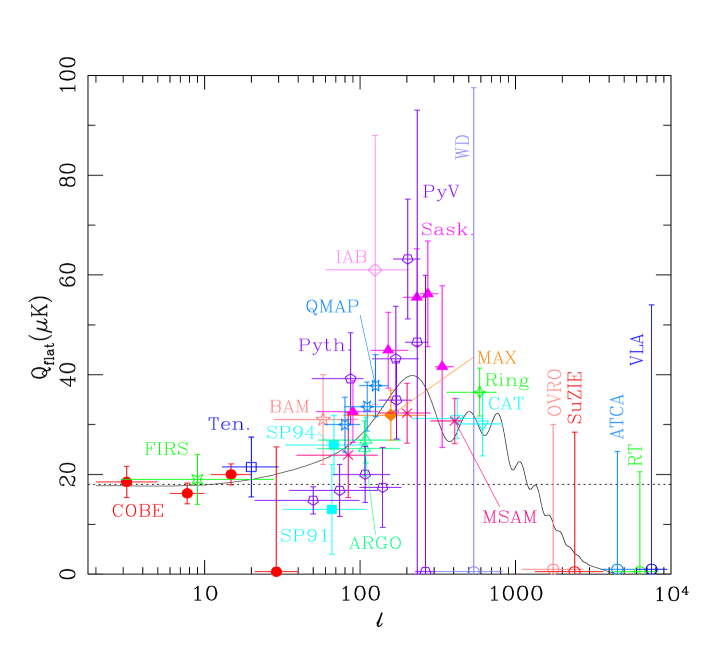
Figure 1.: A summary of the current anisotropy data, here presented as the extrapolated value of the quadrupole moment for a flat power spectrum, plotted against the multipole moment, which is roughly an inverse angle, $\ell\simeq 135^{\circ}/\theta$. The dotted line is the flat power spectrum fit to COBE slone. The solid line is the power spectrum for standard Cold Dark Matter, as an example model. We give a separate list of references at the end, and there are several other recent reviews which discuss current experiments in more detail (e.g. Lawrence 1998).

Despite the steadily improving quality of experiments, we believe that none of the more recent experiments in Figure 1 would have stood as a convincing discovery of primordial anisotropy had it not been for COBE (this remark certainly applies to our own experiment, BAM, as much as to any other experiment). What was critical in the discovery was the understanding of the roles of galactic contributions and systematic errors, provided by COBE’s all-sky coverage and comparatively stable operating environment. It was also crucial for the discovery process that the DMR on COBE and the FIRS balloon program showed a consistent fluctuation amplitude and, later analysis showed, correlated structures observed at very different wavelengths. Many experimenters had reassured themselves by making plots showing the similarity of the FIRS and DMR power spectra, before the end of the day on which the DMR results were announced.

There is a lesson arising from the history of the measurement of the intensity spectrum of the CMB which may be useful here. There were plenty of experiments prior to 1990 which appeared to have sufficient sensitivity to perform useful measurements, many of these with no obvious source of systematic error. The successful 1990 experiments (Gush et al. 1990, Mather et al. 1990) were performed out of the atmosphere, they were differential and they were carried out with a fanatical attention to avoiding systematic errors as the primary design guideline. The results were clear and reliable enough to render moot any lingering debates about inconsistencies between previous experiments. One should not be surprised to see a very similar scenario play itself out in the near term anisotropy measurements.

2. Near Term Future Experiments

Table 1 lists the properties of some future experiments. The list is meant to be illustrative of current planning; experiments are included which are past the proposal stage and for which no results are yet available. Some of the listed experiments already have data. Of course many experiments which have already produced some results and are therefore not on this list will also produce future results. All of the listed experiments involve dedicated, custom-built instrumentation. The control of systematic errors which this allows puts these experiments well ahead of attempts to use existing general purpose facilities.

Table 1.: Several Future Anisotropy Experiments

Snappy	Frequency	$\ell$-range	Number of
Acronym	Coverage (GHz)		freq. channels
Single Dish Telescopes
MAT	26–46, 140–150	30–850	3
MAXIMA	150–420	50–700	4
BOOMERanG	100–800	10–700	4
BEAST	25–90	10–800
TopHat	150–720	10–700	5
ACBAR	150–450	60–2500	4
Interferometers
VSA	26–36	130–1800	6
CBI	26–36	300–3000	10
DASI	26–36	125–700	5
MINT	140–250	1000–3000	10
Satellites
MAP	20–106	1–800	5
Planck	30–850	1–1500	4 + 6

Sufficient sensitivity is achievable, sometimes through great technical effort. The various detection technologies available each impose constraints on experimental design and come with their own set of sources of potential systematic errors. Any serious discussion of specific systematic errors is beyond the scope of this article but we include some naive examples to illustrate the problem. Either a $100\,$mK change in the temperature of an ideal aluminum mirror or a $200\,$mK change in the atmosphere above a stratospheric balloon causes a radiative signal 25 times larger per pixel than the MAP systematic error budget!

2.1. Systematic Errors

The careful CMB experimenter is not paranoid, but knows that the Universe is in fact trying to ruin the experiment. The standard answer to the question of what level of systematic error is tolerable is that there is no systematic way to handle systematic errors and, therefore, that any level of systematic error is a concern. We will ignore this good advice for a moment and try to estimate an answer.

If the goal of an experiment is to get a rough estimate of the power spectrum of the sky, a systematic error amounting to $10\%$ of the signal amplitude contributes about $1\%$ to the power spectrum. Even if the signals are correlated in some surprising way and this estimate is wrong by a factor of a few, the effect is not likely to mask the presence of the main acoustic peak, for example. This fact is what has allowed us to get so far without a better understanding of diffuse foreground sources.

On the other hand, there are important questions whose answer requires correlating many pixels in a map together in order to pick out a fairly weak efect. Measuring amplitudes of non-Gaussian statistics of a map or searching for intensity-polarization correlations are examples. In these cases the requirement for what level of signal systematic errors can contribute to a map becomes very stringent. The amplitude of systematic errors should be below the experiment’s single pixel variance divided by the square root of the number of pixels to be averaged. As a numerical example, in an experiment with $0.13^{\circ}$ pixels and $30\,\mu$K variance averaging 1/10 of the sky, one needs to know that systematic errors are less than $0.06\,\mu$K rms for the average value not to be tainted. This is 50 times better than any experiment we have heard of. The lesson is: to produce maps of the CMB which merit careful scrutiny, avoid systematic errors like the plague.

2.2. Detection Techniques

Detectors fall into two broad categories: coherent detectors, in which the radiative electric field, including its phase, is amplified before detection; and incoherent detectors, which measure total radiative power within some frequency band.

There are two types of very low noise coherent amplifier: InP high electron-mobility transistors (HEMTs); and superconductor-insulator-superconductor (SIS) mixers. HEMTs can be operated at temperatures as warm as room temperature. The noise performance gets better as they are cooled, down to $\simeq 4\,$K, although amplifiers exhibit gain fluctuations at low temperature. Recently HEMT amplifiers have been made to work at frequencies well above $100\,$GHz – noise performance is better at lower frequencies. SIS mixers are typically quieter than HEMTs and can operate at frequencies as high as $1\,$THz. However they must be cooled to $4\,$K to operate. Either of these coherent amplifiers can be used in a single telescope where the signal is amplified and detected, or as part of an interferometer in which case amplified signals from several telescopes are each multiplied with a local oscillator signal yielding lower frequency outputs which are then correlated to produce interference fringes.

The advantages of coherent detectors are that they are fast, stable, not sensitive to microphonic pick-up and involve simple cryogenics. HEMTs also have the important practical advantage that many aspects of detector performance can be verified at room temperature, which greatly speeds up new instrument development. The disadvantage is that they are not as sensitive to broad band signals as incoherent detectors are.

Table 2.: Detection strategies

Snappy	Detectors	Striking	Location
Acronym		Feature
Single Dish Telescopes
MAT	HEMTs and SIS	Has data	Chile 17,000′
MAXIMA	$100\,$mK Bolos.	Has data	Balloon
BOOMERanG	$300\,$mK Bolos.	First CMB LDB flt.	Balloon, LDBa
BEAST			Balloon, LDB
TopHat	Bolometers	Tel. above balloon	Balloon, LDB
ACBAR	$300\,$mK Bolos.	Imaging array	S. Pole 10,000′
Interferometers
VSA	HFETs	14 antennae	Tenerife
CBI	HEMTs at $6\,$K	13 antennae	Chile, 17,000′
DASI	Cooled HEMTs	13 elements	S. Pole, 10,000′
MINT	SIS	6 antennae	Chile
Satellites
MAP	HEMTs $<95\,$K	Differential tels.	Space, L2b
Planck	HEMTs at $20\,$K		Space, L2
	$0.1\,$K Bolos.

Incoherent detectors, in this case bolometers, can be an order of magnitude more sensitive than HEMT and SIS systems. They can be made to operate with background limited performance (BLIP), where fundamental thermodynamic fluctuations in the incident radiation field dominate over detector noise. In addition they can be made to be sensitive to a broad range of wavelengths. However, physical device size scales with wavelength and so it is easier to make small bolometers sensitive. Typically bolometers are designed for frequencies above $50\,$GHz. Bolometers are often susceptible to microphonic and radio-frequency pick-up. They are non-linear and therefore they must be characterized in their experimental operating condition, which can be very difficult for balloon and satellite experiments. They need cumbersome cryogenics to reach their operating temperatures of $0.3\,$K or colder. However, their extraordinary sensitivity and broad frequency coverage often outweigh these disadvantages. Table 2 lists some detector properties for the experiments in Table 1.

Interferometers

The idea of building a dedicated interferometer to study anisotropy of the CMB is not new, but improvements in detectors, and especially in broad bandwidth correlators has made this a very promising option, which is being actively pursued by several groups.

Interferometers do a good job of rejecting the effects of atmospheric variations compared to beam-chopped single telescope instruments. Measurements take place essentially instantaneously, on time scales associated with the interference bandwidth, and on these time scales the atmosphere does not vary. Also, interferometers measure at slightly higher angular resolution than a single telescope of the same overall size, and in any case can easily be built for higher resolution than the currently planned space missions. This advantage will be important in exploring the expected Sunyaev-Zel’dovich forest, especially if they can also be made to work above $200\,$GHz.

Figure 2.: The proposed pointed platform of MINT, with four $30\,$cm aperture telescopes mounted on a single $1.5\,$m platform, illustrating how CMB interferometers are very different from the VLA. Drawing courtesy of W.B. Dorwart, Princeton University.

Unlike the case for conventional radio interferometers, the individual telescopes here are crowded quite close together to keep angular resolution modest. Often, all the telescopes are mounted on a single pointed platform, which eliminates the need for signal delays before the correlators. See White et al. (1997) for an analysis of the performance of these interferometers for measuring anisotropies.

Satellites

Assuming that neither suffers any serious mishap, MAP and Planck will produce definitive measurements of the primary anisotropy of the CMB, at a reliability level which the other experiments can not attain. The reliability arises form the long observation period, complete sky coverage and, primarily, the extraordinarily good observing environment at L2. Even during the 90-odd day period during which it makes its way past the moon and out to L2 to start the nominal observation program, MAP will be in a much more thermally and radiatively stable observing environment than any previous CMB experiment.

3. After MAP and Planck

What will the important experimental questions be after MAP and Planck succeed? Clearly, measurements of the polarization of the CMB, which are explored elsewhere in this volume, will be very exciting. We also expect that studying diffuse foreground emission will become very exciting and active, as our ability to measure and identify these sources of emission develops. However, that topic is covered in the whole rest of this book so we need not consider it further here! For the remainder of this article we will discuss various ideas for what might be conceivable in the more long term future.

3.1. Anisotropy

Statistics

Can phases contain information which is not more easily seen in the power spectrum? In principle, of course the answer is yes. But in practice, it seems clear that the smart money has to be on the negative answer. So although it would always be foolish to neglect to search for other signals, we expect that the vast majority of the primary anisotropy information will be contained in the power spectrum. Partly this is because the signals seem likely to be close to Gaussian, but also because the power spectrum (or the variance as a function of scale) is such a robust quantity – specific patterns on the sky may require lots of phase-correlation to produce them, but much of that simply specifies the specific realization, rather than containing information about the underlying model. The supremacy of the power spectrum will certainly cease to be true for foreground signals, or indeed for a range of astrophysical processing effects that come in at smaller angular scales.

One could imagine mounting a specific search for, e.g. point or line sources on the sky, as specific examples of non-Gaussian signals. One question to ask, then, is what sort of strategy one would design to carry this out most efficiently (and convincingly). We find it hard to see how to avoid the conclusion that you would end up making a map, perhaps deeper and with higher resolution than otherwise, but a map nevertheless. Hence we suspect that the search for non-Gaussian signals is unlikely to be a strong driver for the design of future experiments, even if it plays a stronger role in the data analysis.

A great deal of effort has been going into the study of non-Gaussian signals, e.g. using Minkowski functionals, wavelets, etc. Given how many such tests have already been applied to COBE, we imagine that every reasonable statistic will be measured for all future large data-sets. In particular we foresee an increased interest in the investigation of non-Gaussian statistics for various sorts of foreground signal.

Angular scales

Ignoring foregrounds, how far out in $\ell$ is far enough? Planck seems sufficient for the primary signal. But that may change, depending on what we learn about foregrounds and the secondary signals, caused by various astrophysical effects, which conceptually lie in the ‘grey-area’ between background and foregrounds. There seems to be a growing interest in these astrophysical signals at small scales, and we see no reason for that to change. It may be that the smallest angular scales are ultimately best probed with interferometers. We expect there to be secondary signal information down to the angular scales of distant galaxies, i.e. $\ell\simeq{\rm few}\times 10^{4}$.

A CMB Deep Field

What might we learn from a CMB deep field? Of course, irrespective of the answer to that question, it will be done anyway! Non-Gaussian signals from higher-order effects at small-scales would certainly show up in such a map. On scales where there has been significant growth of structure, and certainly on non-linear scales, we would expect there to be significant non-Gaussianity. There seems little doubt that at some point, when the instrumentation has matured, it will be worthwhile to carry out such a CMB Deep Field. Exactly how non-Gaussian (or in other ways surprising) the small-scale signals turn out to be will determine how far beyond ‘cosmic variance’ it is worth integrating.

Sunyaev-Zel’dovich effects

We are sure that, motivated by the impressive results of today’s experimenters, investigation of S-Z effects will continue to grow as a sub-field. Particularly exciting is the idea of ‘blank sky’ searches for the ‘S-Z Forest’, or ionized gas tracing out the Cosmic Web.

The thermal Sunyaev-Zel’dovich effect, or inverse Compton scattering of the CMB photons through hot gas, gives a temperature fluctuation of roughly $(kT_{\rm e}/m_{\rm e}c^{2})\tau$, where $T$ and $m_{\rm e}$ are the temperature and mass of the electron, respectively, and $\tau$ is the optical depth through the ionized gas. There is also a spectral shape, distinct from the CMB blackbody, of a well-known form (see e.g. Sunyaev & Zel’dovich 1980) Detailed studies of the thermal S-Z effect for particular clusters will provide constraints on the morphology, clumping, thermal state of the gas and projected mass, amongst other things. The power spectrum of these fluctuations peaks at $\ell\simeq 2000$ typically, with $\left\langle Q_{\rm flat}\right\rangle$ amplitude of a few $\mu$K, although with great variation between models. Detailed investigation of this power spectrum might further distinguish between cosmological models, and between ideas for cluster formation. The power spectrum for the kinematic effect, and for related effects (due to variations in potential, for example) are generally much smaller.

Several of these ‘higher-order’ Sunyaev-Zel’dovich type effects are potentially measurable for individual clusters, and will doubtless be attempted in the future (see the review by Birkinshaw 1998). Certainly the kinematic effect (which depends on the line-of-sight velocity and is $\sim(v_{\parallel}/c)\tau$) can be measured for some clusters. However, this effect has the same spectrum as a CMB fluctuation, and so the small-angle CMB anisotropies act as a source of ‘noise’, making is difficult to measure the velocities to better than a few hundred ${\rm km}\,{\rm s}^{-1}$. One further effect uses the polarization in the CMB scattered by the kinematic S-Z effect, which depends on the cluster’s transverse velocity (actually $\sim(v^{2}/c^{2})\tau$). In principle, together with the kinematic S-Z effect itself, this gives a means of estimating the full 3 dimensional velocity of clusters. Although difficult to measure, this polarization signal has a frequency dependence which may help to disentangle it from other effects (Audit & Simmons 1999). There are other spectral signals expected from non-thermal electron populations, for example in the lobes of radio sources. However, the utilisation of such measurements to study the lobe properties will require extremely high angular resolution.

Other secondary effects

There are several other known secondary effects (see, e.g. Hu et al. 1995, and other contributions to this volume), and surely many other unknown ones!

One effect which has been studied in some detail is a second-order coupling between density and velocity, usually referred to as the Vishniac effect. In a sense this can be thought of as specific case of the kinematic Sunyaev-Zel’dovich effect. For Cold Dark Matter type models the signal is typically $\simeq 1\,\mu$K and peaking at $\ell\simeq{\rm few}\times 10^{3}$ (e.g. Hu & White 1996, Jaffe & Kamionkowski 1998). Although certainly difficult to measure, it is nevertheless feasible, and worth pursuing, since measurement can give direct information about reionization. Additional structure ar small scales (e.g. from an isocurvature mode) could increase the signal. In addition there will be polarization effects, although these are likely to be really small.

Patchy reionization (discussed elsewhere in this volume) is just another S-Z effect, and tends to be dominated by the kinematic source from moving bubbles of gas as the Universe undergoes reionization. The amplitude of this signal seems likely to be smaller than for the Vishniac effect, although it is as yet unclear what the predictions will be for realistic models which include inhomogeneous reionization (with radiative transfer through voids etc.), distributions of sources, and other complications. Again there may be polarization effects, and correlations with other signals, which, in principle, could be used to pull the signal out. In addition there may also be a measurable S-Z signal from the Ly$\,\alpha$ forest, on scales well below an arcminute, and with amplitude perhaps as high as a few $\mu$K (Loeb 1996).

Rees-Sciama, or varying potential fluctuations tend to be rather small in amplitude ($<10^{-6}$ in fractional temperature change), but not negligibly so. Here again there are a number of effects, in particular those caused by time-varying potentials in the light-crossing time, and those caused by potentials moving across the line of sight (e.g. Tuluie, Laguna & Anninos 1996). These will have CMB-like spectra, and the signal will be dominated by non-linear structures (meaning that the statistics will be highly non-Gaussian). The effects may peak at relatively small angles $\ell\simeq{\rm few}\times 100$, but there they will be well below the primary signal, and hard to disentangle. So the best prospects for detection may be at smaller scales, where the primary power spectrum is falling off. Detection may also be easier using correlations with other signals. And certainly such signals are unlikely to be Gaussian, and so may be teased out of the data by looking at their statistics (e.g. Spergel & Goldberg 1999).

Gravitational lensing affects the CMB power spectrum by smearing the anisotropies, thereby smoothing out features in the power spectrum. The temperature field is affected by this smearing, so that combinations of derivatives can be used to extract the lensing signal directly, at least in principle (Seljak & Zaldarriaga 1999). The projected matter field can be reconstructed through a combination of this technique and correlations with other signals (Zaldarriaga & Seljak 1999). For example, the large angle signal caused by the variation in gravitational potential (the ‘ISW effect’) may be correlated with the lensing signal in open or $\Lambda$-dominated models. However, the level of such a correlated signal is not likely to be large. One can easily imagine searching for all sorts of other correlations, for example the lensing signal with S-Z signals, with surveys at other wavelengths, e.g. large-scale structure, X-ray maps, etc.

Spatial-spectral signals

At the moment the only significant signal which mixes both spatial and spectral deviations is the S-Z effect. Although we have no specific ideas, we imagine that other such effects, involving perhaps different scattering processes, are likely to be developed in the near future. Although we expect the effect to be quite small, we mention as an example that Rayleigh scattering, which would spectrally filter anisotropy signals, has been omitted from calculations. In addition there could in principle be resonant line scattering from molecules in clouds at high redshift. Searches for such mixed spatial-spectral signals seem likely to become more important as multi-frequency data-sets improve in quality and quantity.

3.2. Non-anisotropy

Non-anisotropy measurements are heroically hard to do; certainly such things are worth pursuing, but the immediate returns are not as obvious as for the current anisotropy prospects. On the other hand, we expect that effort will fairly soon return to this direction when the ‘easy’ results have been mined from the primary power spectrum. Here we simply list a number of possibilities. Figure 3 shows the form of some of the standard distortions to the CMB spectrum.

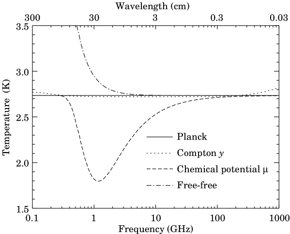
Figure 3.: Shapes for some theoretical possibilities for spectral distortions. The amplitudes here are arbitrary. However, the FIRAS 95% confidence limits for the amplitudes of these distortions are that the chemical potential is less than $15\,$mK at the peak and that free-free is less than $10\,$mK at $4\,$GHz. At those frequencies the Galaxy is perhaps 100 times brighter. See Smoot (1997) for further discussion.

A FIRAS/COBRA style total emission measurement of the spectrum of the sky will almost entirely be dominated by foregrounds outside of the 20 to $400\,$GHz frequency window in which the spectrum is already well measured. The present FIRAS limits allow parametrized spectral distortions as large as 10s of mK, easily larger than the measurement uncertainty in a careful experiment, but 100 to 1000 times dimmer than diffuse galactic emission at those wavelengths! Perhaps a multi-frequency measurement with appropriate angular resolution and sky coverage will allow a reliable extrapolation to zero galactic emission, but it will not be easy. Details for commonly considered distortions are listed below.

Compton distortions

$y$-distortions have essentially already been measured, in the sense that the sum of all the S-Z detected structure will give the uniform Compton-distortion over the sky. Certainly this gives a lower limit, which seems likely to be the bulk of the detectable signal (barring unforeseen exotic processes). The size of this signal is estimated to be $y\sim 10^{-6}$ (e.g. Colafrancesco et al. 1997), depending on the cosmology. After the Planck mission (and S-Z investigations from ground-based interferometers) we will have a very precise estimate for the uniform $y$-distortion (and indeed an estimate of its power spectrum as well). Between this underlying signal, and the FIRAS upper limit on a full-sky distortion, there will remain only a rather narrow window to search for possible isotropic $y$-distortions from other sources (such as late energy injection, unrelated to cluster formation). Since there are no immediate candidates for such processes, and the window is rather narrow, we don’t see this as a particularly strong motivation for mounting a next generation FIRAS mission.

Free-free emission

For late energy releases, free-free emission leads to a distortion in the CMB spectrum, which increases towards lower frequency. This seems to be the type of distortion which is most feasible to measure in the near future for realistic models of the Universe. The best upper limits at the moment imply free-free optical depths of order $Y_{\rm ff}\mathrel{\hbox{\hbox to0.0pt{\hbox{\lower 4.0pt\hbox{$\sim$}}\hss}\hbox{$<$}}}10^{-5}$ (e.g. Nordberg & Smoot 1998). Since this distortion increases at lower frequencies, then it is best investigated at the lowest frequency at which foreground signals can be dealt with, which means somewhere around $5\,$GeV. The expected signal at these frequencies may be as high as $100\,\mu$K, corresponding to $Y_{\rm ff}$ only about an order of magnitude below the current limits. The planned experiments ARCADE and DIMES (Kogut 1996) may be able to reach into the parameter space for realistic models, and help us understand more about the early ionized stages of the intergalactic medium. One nice thing about free-free is that lowering the temperature of the ionized medium increases the distortion (approximately $\propto n_{\rm e}^{2}/\sqrt{T_{\rm e}}$), even although it decreases the Compton distortion. Hence good limits on $Y_{\rm ff}$ imply either low reionization redshifts or high electron temperatures, and limits on $y$ would restrict $T_{\rm e}$, so that direct limits on $z_{\rm reion}$ could be obtained.

Chemical potential

Current limits on $\mu$-type distortions are at the $10^{-5}$ level. Note that this allows about $15\,$mK at $1\,$GHz within the error budget of the measurements, which is about 0.1% of the galactic signal. So pushing that limit further down is going to be tricky! The way to do this would presumably be to make a spectral map of the sky and extrapolate to zero galaxy (essentially what FIRAS did). So how big could a signal be?

Some amount of $\mu$-distortion is unavoidable, since it is generated by the damping of small-scale perturbations. For realistic models the value is likely to be around ${\rm few}\times 10^{-8}$ (Hu, Scott & Silk 1994), which seems unlikely ever to be measurable. Of course various exotic processes, including energy injection at redshifts $z\sim 10^{5}$ could give much higher values of $\mu$. Limits could be set by experiments which also constrain free-free signals. However, we see no compelling reason currently to invest heavily in future experiments seeking to measure $\mu$ itself. Of course, if any hint of signal were to turn up then that would be extremely exciting (since unexpected) – in that case further investigation of the turn-off in the distortion at low frequencies would probe an otherwise unexplored early epoch.

Recombination lines

When the Universe recombined, every atom emitted at least one Lyman photon, or else got from the first excited state to the ground state via the two-photon process (see Seager, Scott & Sasselov 1999 for more details). This is a lot of photons, waiting there to be discovered! Mere measurement of the background of these photons would be an unprecedented confirmation of the Big Bang paradigm, that the Universe became neutral at $z\simeq 1000$. Further investigation of these recombination lines would be a direct probe of the recombination process, and might provide further cosmological constraints. For example, the strengths of the residual Ly$\,\alpha$ feature and the two-photon feature will depend on the baryon density and on the expansion rate, hence allowing measurements of $\Omega_{\rm B}$ and $H$ at $z\simeq 1000$.

The problem is that the main recombination lines lie at wavelengths $\lambda\simeq 150\,\mu$m, where the signal from the galaxy is orders of magnitude stronger. The way to try to find the signal is then presumably to have enough spatial information to be able to extrapolate to zero Galaxy, and at the same time to have adequate spectral information to distinguish the relatively wide spectral feature. If all else failed it might be possible to rely on the dipole to extract the cosmological signal, but that would be even more difficult. So we might envisage an experiment with reasonable sky coverage, low angular resolution, but at least 3 spectral channels (say in the range 100–200$\,\mu$m) to extract the wide line. The spectral resolution would have to be good enough to distinguish this from a roughly isotropic component of warm interstellar dust – but that should be possible given that the spectral shape of the recombination lines is calculable (Dell’Antonio & Rybicki 1993, Boschan & Biltzinger 1998).

21 cm line studies

If the Universe became reionized at redshifts between 5 and 20 there should be a spectral feature due to red-shifted $21\,$cm emission from neutral hydrogen which appears today at $70$ to $240\,$MHz (see Shaver et al. 1999). This emission can be seen against the CMB provided that there are spatial or spectral signatures (e.g. Tozzi, et al. 1999) and a mechanism which decoupled the electron spin temperature from the CMB. In principle, such studies, using the proposed Square Kilometer Array for example, could provide information about the processes that marked the end of the so-called Dark Ages, i.e. the reionization process and the formation of the first structures. This endeavor is sometimes called ‘cosmic tomography’.

Other diagnostics of the ‘Dark Ages’

There are of course other ways of probing the end of the Dark Ages, and even into that epoch, many of which might come from entirely different wavelengths, for example the near infra-red with NGST. However, we imagine that the microwave band will continue to be important in furnishing new ideas for exploring the domain between $z=5$ and $z=1000$. One recent speculative idea involves searching for masers which may come from structures at either the recombination or reionization epochs (Spaans & Norman 1997). There will surely be other such ideas in the coming years.

Measurements of $T_{\rm CMB}(z)$

The currently best value for the CMB temperature is $T_{0}=2.725\pm 0.001\,$K (Mather et al. 1999). It seems unclear why anyone should care about a more precise measurement than that! Before the existence of the CMB was even suspected, there was evidence for excess excitation in line ratios of certain molecules, notably cyanogen , in the interstellar medium (McKellar, 1941). This method has more recently been used to constrain the CMB temperature at high redshifts ($z\sim{\rm few}$) using line with excitation temperatures of the relevant energy (e.g. Songaila et al. 1994, Roth & Bauer 1999). Measurements of other line ratios etc. can be used to set limits on the variation of fundamental physical constants (e.g. Webb et al. 1999). In a similar way, detailed measurement of the blackbody shape indicates that certain combinations of fundamental constants have not varied much since $z\sim 1000$.

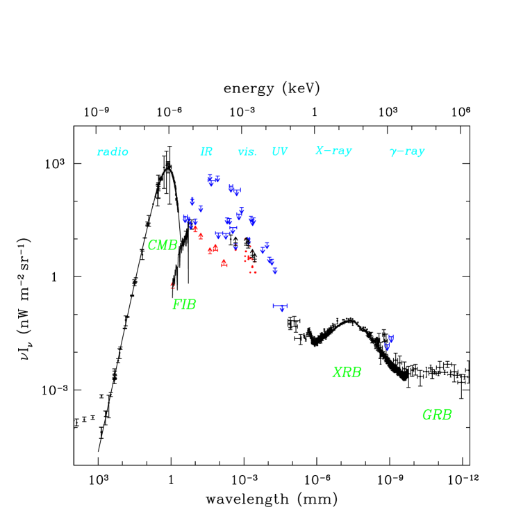
Figure 4.: A compilation of recent constraints on extragalactic diffuse background radiation. In terms of total energy the CMB and Far-Infrared Backgrounds dominate. The data are collected primarily from Ressel & Turner 1990, Smoot 1997, Lagache et al. 1999, Hauser et al. 1998, Dwek & Arendt 1998, Pozzetti et al. 1998, Leinert et al. 1998, Miyaji et al. 1998, Sreekumar et al. 1998, and Kappadath et al. 1999. In this colour version lower limits are shown in red and upper limits in blue.

4. Epilogue

Assuming that MAP and Planck are fully successful, and that the current suite of ground- and balloon-based experiments also return exquisite data, what then? Will this be then end of the study of the CMB? Eventually we can imagine a time when the primordial anisotropies have been measured so accurately that there are diminishing returns from further generations of satellite missions, and when small scale measurements, involving non-Gaussian signals, mixed spatial-spectral signals, and other complications, have moved firmly into the regime of ‘messy astrophysics’. However, there will be further primordial information to unlock from ever more ambitious polarization experiments. Certainly the CMB should not be looked at in isolation – although it is the dominant diffuse extragalactic background, there are several others to study (see Figure 4). And if that doesn’t leave the future still filled with exciting and challenging possibilities, there’s always the cosmic neutrino background!

Acknowledgments.

We thank the editors for their patience.

References

Audit, E., & Simmons, J. F. L., 1999, MNRAS, submitted, [astro-ph/9812310]

Birkinshaw, M, 1999, Physics Reports, in press [astro-ph/9808030]

Bond, J. R., Jaffe, A. H., & Knox, L. E., 1998, ApJ, in press, [astro-ph/9808264]

Boschán, P., & Biltzinger, P., 1998, A&A, 336, 1

Colafrancesco, S., Mazzotta, P., Rephaeli, Y., & Vittorio, N., 1997, ApJ, 479, 1 [astro-ph/9703121]

Dell’Antonio, I. P., & Rybicki, G. B., 1993, in ‘Observational Cosmology’, ASP Conf. Ser. Vol. 51

Dwek, E., & Arendt, R. G., 1998, ApJ, 508, L9

Gush, H. P., Halpern, M., & Wishnow, E. H., 1990, Phys Rev. Lett., 65, 537

Hauser, M. G., et al., 1998, ApJ, 508, 25

Hu, W., Scott, D., & Silk, J., 1995, ApJ, 430, L5 [astro-ph/9402045]

Hu, W., Scott, D., Sugiyama, N., & White, M., 1995, Phys. Rev., D52, 5498 [astro-ph/9505043]

Hu, W., & White, M., 1996, A&A, 315, 33 [astro-ph/9507060]

Jaffe, A. H., & Kamionkowski, M., 1998, Phys. Rev., D58, 43001 [astro-ph/9801022]

Kappadath, S. C., et al., 1999, HEAD, 31, 3503

Kogut, A., 1996, in Proc. XVI Moriond Astrophysics meeting [astro-ph/9607100]

Lagache, G., Abergel, A., Boulanger, F., Désert, F. X., & Puget, J.-L., A&A, 344, 322 [astro-ph/9901059]

Lawrence, C. L., 1998, in ‘Evolution of Large Scale Structure’, ed. A.J. Banday et al., in press,

Lawrence, C. L., Scott, D., & White, M., 1999, PASP, in press, [astro-ph/9810446]

Leinert, C. H., et al., 1998, A&AS, 127, 1

Loeb, A., 1996, ApJ, 471, L1 [astro-ph/9511075]

Mather, J. C., et al., 1990, ApJ, 354, L37

Mather, J. C., Fixsen, D., Shafer, R. A., Mosier, C., & Wilkinson, D. T., 1999, ApJ, 512, 511 [astro-ph/9810373]

McKellar, A., 1941, Publ. Dom. Astrophys. Obs, Victoria, B.C., 7, 251

Miyaji, T., et al., 1998, A&A, 334, L13

Nordberg, H. P., & Smoot, G. F., 1998, ApJ, submitted [astro-ph/9805123]

Pozzetti, L., et al., 1998, MNRAS, 298, 1133

Roth, K. C., & Bauer, J. M., 1999, ApJ, 515, L57

Seager, S., Sasselov, D., & Scott, D., 1999, ApJ, submitted

Seljak, U., & Zaldarriaga, M., 1999, Phys. Rev. Lett., 82, 2636 [astro-ph/9810092]

Shaver, P. A., Windhorst, R. A., Madau, P., & de Bruyn, A. G., 1990, A&A, submitted [astro-ph/9901320]

Smoot, G. F., 1997, Proc. of the Strasbourg NATO School, in press [astro-ph/9705101]

Smoot, G. F., & Scott, D., 1998, in Caso C., et al., Eur. Phys. J., C3, 1, the Review of Particle Physics. p.$\,127$ [astro-ph/9711069]

Songaila, A., et al., 1994, Nature, 371, 43

Spaans, M., & Norman, C. A., 1997, ApJ, 483, 87

Spergel, D. N., & Goldberg, D. M., 1999, ApJ, in press [astro-ph/9811252]

Sreekumar, P., et al., 1998, ApJ, 494, 523

Sunyaev, R. A., & Zel’dovich, Ya. B., 1980, ARAA, 18, 537

Tozzi, P., Madau, P., Meiksin, A., & Rees, 1999, ApJ, submitted [astro-ph/9903139]

Tuluie, R., Laguna, P., & Anninos, P., 1996, ApJ, 463, 15

Webb, J. K., et al., 1999, Phys. Rev. Lett., 82, 884

White, M., Carlstrom, J. E., Dragovan, M., & Holzapfel, S. W. L., 1997, ApJ, in press [astro-ph/9712195]

Zaldarriaga, M., & Seljak, U., 1999, Phys. Rev. D, in press [astro-ph/9810257]

Anisotropy Results

COBE: Hinshaw, G. et al., 1996, ApJ, 464, L17

FIRS: Ganga, K., Page, L., Cheng, E., & Meyers, S., 1993, ApJ, 432, L15

Ten.: Gutiérrez, C. M., et al., 1997, ApJ, 480, L83

BAM: Tucker, G. S., et al., 1997, ApJ, 475, L73

SP91: Schuster, J., et al., 1993, ApJ, 412, L47 (Revised, see SP94 reference)

SP94: Gundersen, J. O., et al., 1994, ApJ, 443, L57

Sask.: Netterfield, et al., 1997, ApJ, 474, 47

Pyth.: Platt, S. R., et al., 1997, ApJ, 475, L1

PyV: Coble, K., et al., 1999, ApJ, in press [astro-ph/9902195]

ARGO: de Bernardis, P., et al., 1994, ApJ, 422, L33; Masi, S., et al., 1996, ApJ463, L47

QMAP: de Oliveira-Costa, A., et al., 1998, ApJ, 509, L77; Herbig, T., et al., 1998, ApJ, 509, L73; Devlin, M., et al., 1998, ApJ, 509, L69

IAB: Piccirillo, L., & Calisse, P., 1993, ApJ, 413, 529

MAX: Tanaka, S. T., et al., 1996, ApJ, 468, L81; Lim, M., et al., 1996, ApJ, 469, L69

MSAM: Cheng, E. S., et al., 1996, ApJ, 456, L71; Cheng, E. S., et al., 1997, ApJ, 488, L59; Wilson, G. W., et al., ApJ, in press [astro-ph/9902047]

CAT: Scott, P. F. S., et al., 1996, ApJ, 461, L1; Baker, J. C., 1997, Proc. Particle Physics and Early Universe Conf., (http://www.mrao.cam.ac.uk/ peuc/astronomy/papers/baker/baker.html); Baker, J. C., et al., in preparation

WD: Tucker, G. S., Griffin, G. S., Nguyen, H. T., & Peterson, J. B., 1993, ApJ, 419, L45; Ratra, B., et al., 1998, ApJ, 505, 8

OVRO: Readhead, A. C. S., et al., 1989, ApJ, 346, 566

Ring: Leitch, E. M., et al., 1998, ApJ, in press [astro-ph/9807312]

SuZIE: Church, S. E., et al., 1997, ApJ, 484, 523

ATCA: Subrahmayan, R., Ekers, R. D., Sinclair, M., & Silk, J., 1993, MNRAS, 263, 416

RT: Jones, M. E., 1997, Proc. Particle Physics and Early Universe Conference (http://www.mrao.cam.ac.uk/ ppeuc/astronomy/papers/jones/jones.html); Jones, M. E., et al., in preparation

VLA: Partridge, B., et al., 1997, ApJ, 483, 38