Application of Wavelets to Filtering of Noisy Data

Abstract

wavelets, optimal filtering, wiener filtering I discuss approaches to optimally remove noise from images. A generalization of Wiener filtering to Non-Gaussian distributions and wavelets is described, as well as an approach to measure the errors in the reconstructed images. We argue that the wavelet basis is highly advantageous over either Fourier or real space analysis if the data is intermittent in nature, i.e. if the filling factor of objects is small.

1 Introduction

In astronomy, the collection of data is often limited by the presence of background noise. Various methods are used to filter the noise while retaining as much “useful” information as possible. In recent years, wavelets have played an increasing role in astrophysical data analysis. It provides for a general parameter-free procedure to look for objects of varying size scales. In the case of the Cosmic Microwave Background (CMB) one is interested in the non-Gaussian component in the presence of Gaussian noise and signal. An application of wavelets is presented by Tenorio et al (1999). This paper generalizes their analysis beyond the thresholding approximation. X-ray images are also frequently noise dominated, caused by instrumental and cosmic background. Successful wavelet reconstructions were achieved by Damiani et al (1997a,b).

At times generic tests for non-Gaussianity are desired. Inflationary theories predict, for example, that the intrinsic fluctuations in the CMB are Gaussian, while topological defect theories predict non-Gaussianity. A full test for non-Gaussianity requires measuring all N-point distributions, which is computationally not tractable for realistic CMB maps. Hobson et al (1998) have shown that wavelets are a more sensitive discriminant between cosmic string and inflationary theories if one examines only the one point distribution function of basis coefficients.

For Gaussian random processes, Fourier modes are statistically independent. Current theories of structure formation start from an initially linear Gaussian random field which grows non-linear through gravitational instability. Non-linearity occurs through processes local in real space. Wavelets provide a natural basis which compromise between locality in real and Fourier space. Pando & Fang (1996) have applied the wavelet decomposition in this spirit to the high redshift $L_{\alpha}$ systems which are in the transition from linear to non-linear regimes, and are thus well analyzed by the wavelet decomposition.

We will concentrate in this paper on the specific case of data layed out on a two dimensional grid, where each grid point is called a pixel. Such images are typically obtained through various imaging instruments, including CCD arrays on optical telescopes, photomultiplier arrays on X-ray telescopes, differential radiometry measurements using bolometers in the radio band, etc. In many instances, the images are dominated by noise. In the optical, the sky noise from atmospheric scatter, zodiacal light, and extragalactic backgrounds, sets a constant flux background to any observation. CCD detectors essentially count photons, and are limited by the Poissonian discreteness of their arrival. A deep exposure is dominated by sky background, which is subtracted from the image to obtain the features and objects of interest. Since the intensity of the sky noise is constant, it has a Poissonian error with standard deviation $e\propto n^{1/2}$, where $n$ is the photon count per pixel. After subtracting the sky average, this fluctuating component remains as white noise in the image. For large modern telescopes, images are exposed to near the CCD saturation limit, with typical values of $n\sim 10^{4}$. The Poisson noise is well described by Gaussian statistics in this limit.

We would like to pose the problem of filtering out as much of the noise as possible, while maximally retaining the data. In certain instances, optimal methods are possible. If we know the data to consist of astronomical point objects, which have a shape on the grid given by the atmospheric spreading or telescope optics, we can test the likelihood at each pixel that a point source was centered there. The iterative application of this procedure is implemented in the routine clean of the Astronomical Image Processing Software (AIPS) (Cornwell & Braun 1989).

If the sources are not point-like, or the atmospheric point spread function varies significantly across the field, clean is no longer optimal. In this paper we examine an approach to implement a generic noise filter using a wavelet basis. In section 2 we first review two popular filtering techniques, thresholding and Wiener. In section 3 we generalize Wiener filtering to inherit the advantages of thresholding. A Bayesian approach to image reconstruction (Vidakovic 1998) is used, where we use the data itself to estimate the prior distribution of wavelet coefficients. We recover Wiener filtering for Gaussian data. Some concrete examples are shown in section 4.

2 Classical Filters

2.1 Thresholding

A common approach to supressing noise is known as thresholding. If the amplitude of the noise is known, one picks a specific threshold value, for example $\tau=3\sigma_{\rm noise}$ to set a cutoff at three times the standard deviation of the noise. All pixels less than this threshold are set to zero. This approach is useful if we wish to minimize false detections, and if all sources of signal occupy only a single pixel. It is clearly not optimal for extended sources, but often used due to its simplicity. The basic shortcoming is its neglect of correlated signals which covers many pixels. The choice of threshold also needs to be determined heuristically. We will attempt to quantify this procedure.

2.2 Wiener Filtering

Figure 1: The power spectrum of figure 3. The dashed line is the power spectrum measured from the noisy data. The horizontal line is the noise. The lower solid line is the difference between the measured spectrum and the noise. We see that the measurement of the difference becomes noise limited at large $k$.

In the specific case that both the signal and the noise are Gaussian random fields, an optimal filter can be constructed which minimizes the impact of the noise. If the noise and signal are stationary Gaussian processes, Fourier space is the optimal basis where all modes are uncorrelated. In other geometries, one needs to expand in signal-to-noise eigenmodes (see e.g. Vogeley and Szalay 1996). One needs to know both the power spectrum of the data, and the power spectrum of the noise. We use the least square norm as a measure of goodness of reconstruction. Let $E$ be the reconstructed image, $U$ the original image and $N$ the noise. The noisy image is called $D=U+N$. We want to minimize the error $e=\langle(E-U)^{2}\rangle$. For a linear process, $E=\alpha D$. For our stationary Gaussian random field, different Fourier modes are independent, and the optimal solution is $\alpha=\langle U^{2}\rangle/\langle D^{2}\rangle$. $U^{2}$ is the intrinsic power spectrum. Usually, $D^{2}$ can be estimated from the data, and if the noise power spectrum is known, the difference can be estimated subject to measurement scatter as shown in figure 1. Often, the powerspectrum decays with increasing wave number (decreasing length scale): $\langle U^{2}\rangle=ck^{-n}$. For white noise with unit variance, we then obtain $\alpha=c/(k^{n}+c)$, which tends to one for small $k$ and zero for large $k$. We really only need to know the parameters $c,n$ in the crossover region $E^{2}\sim 1$. In section 4 we will illustrate a worked example.

Wiener filtering is very different from thresholding, since modes are scaled by a constant factor independent of the actual amplitude of the mode. If a particular mode is an outlier far above the noise, the algorithm would still force it to be scaled back. This can clearly be disadvantageous for highly non-Gaussian distributions. If the data is localized in space, but sparse, the Fourier modes dilute the signal into the noise, thus reducing signal significantly as is seen in the examples in section 4. Furthermore, choosing $\alpha$ independent of $D$ is only optimal for Gaussian distributions. One can generalize as follows:

3 Non-Gaussian Filtering

We can extend Wiener filtering to Non-Gaussian Probability Density Functions (PDFs) if the PDF is known and the modes are still statistically independent. We will denote the PDF for a given mode as $\Theta(u)$ which describes a random variable $U$. When Gaussian white noise with unit variance ${\cal N}(0,1)$ is added, we obtain a new random variable $D=U+{\cal N}(0,1)$ with PDF $f(d)=(2\pi)^{-1/2}\int\Theta(u)\exp(-(u-d)^{2}/2)du$. We can calculate the conditional probability $P(U|D)=P(D|U)P(U)/P(D)$ using Bayes’ theorem. For the posterior conditional expectation value we obtain

$$\langle U|D=d\rangle = \frac{1}{\sqrt{2\pi}f(d)}\int\exp[-(u-d)^{2}/2]\Theta(u)udu$$ (1)

$$= D+\frac{1}{\sqrt{2\pi}f(d)}\partial_{d}\int\exp[-(u-d)^{2}/2]\Theta(u)du$$

$$= D+(\ln f)^{\prime}(d).$$

Similarly, we can calculate the posterior variance

$$\left\langle(U-\bar{U})^{2}|D=d\right\rangle=1+(\ln f)^{\prime\prime}(d).$$ (2)

For a Gaussian prior with variance $\sigma$, equation (1) reduces to Wiener filtering. We have a generalized form for $\alpha=1+(\ln f)^{\prime}/D$. For distributions with long tails, $(\ln f)^{\prime}\sim 0$, $\alpha\sim 1$, and we leave the outliers alone, just as thresholding would suggest.

For real data, we have two challenges:

1. estimating the prior distribution $\Theta$.

2. finding a basis in which $\Theta$ is most non-Gaussian.

3.1 Estimating Prior $\Theta$

The general non-Gaussian PDF on a grid is a function of $N$ variables, where $N$ is the number of pixels. It is generally not possible to obtain a complete description of this large dimensional space (D. Field, this proceedings). It is often possible, however, to make simplifying assumptions. We consider two descriptions: Fourier space and wavelet space. We will assume that the one point distributions of modes are non-Gaussian, but that they are still statistically independent. In that case, one only needs to specify the PDF for each mode. In a hierarchical basis, where different basis functions sample characteristic length scales, we further assume a scaling form of the prior PDF $\Theta_{l}(u)=l^{-\beta}\Theta(u/l^{\beta})$. Here $l\sim 1/k$ is the characteristic length scale, for example the inverse wave number in the case of Fourier modes. For images, we often have $\beta\sim 1$.

Wavelets still have a characteristic scale, and we can similarly assume scaling of the PDF. In analogy with Wiener filtering, we first determine the scale dependence. For computational simplicity, we use Cartesian product wavelets (Meyer 1992). Each basis function has two scales, call them $2^{i},2^{j}$. The real space support of each wavelet has area $A\propto 2^{i+j}$, and we find empirically that the variance depends strongly on that area. The scaling relation does not directly apply for $i\neq j$, and we introduce a lowest order correction using $\ln(\sigma)=c_{1}(i+j)+c_{2}(i-j)^{2}+c_{3}$. We then determine the best fit parameters $c_{i}$ from the data. The actual PDF may depend on the length scale $i+j$ and the elongation $i-j$ of the wavelet basis. One could parameterize the PDF, and solve for this dependence (Vidakovic 1998), or bin all scales together to measure a non-parametric scale averaged PDF. We will pursue the latter.

The observed variance is the intrinsic variance of $\Theta$ plus the noise variance of ${\cal N}$, so the variance $\sigma_{\rm intrinsic}^{2}=\sigma_{\rm obs}^{2}-\sigma_{\rm noise}^{2}$ has error $\propto\sigma_{\rm obs^{2}}/n$ where $n$ is the number of coefficients at the same length scale. We weigh the data accordingly. Because most wavelet modes are at short scales, most of the weight will come near the noise threshold, which is what we desire. We now proceed to estimate $f(d)$. Our Ansatz now assumes $\Theta_{ij}(u)\propto\Theta(u/\exp[c_{1}(i+j)+c_{2}(i-j)^{2}+c_{3}])$ where $\Theta(u)$ has unit variance. We can only directly measure $f_{ij}$. We sort these in descending order of variance, $f_{m}$. Again, typically the largest scale modes will have the largest variance. In the images explored here, we find typical values of $c_{1}$ between 1 and 2, while $c_{2}\sim-0.2$. For the largest variance modes, noise is least important. From the data, we directly estimate a binned PDF for the largest scale modes. By hypothesis, $D=U/l^{\beta}+{\cal N}(0,\sigma_{l,\rm noise})$. We reduce the larger scale PDF by convolving it with the difference of noise levels to obtain an initial guess for the smaller scale PDF:

$$f^{\prime}_{l^{\prime}}(d)=\frac{(l^{\prime}/l)^{\beta}}{\sqrt{\pi}}\int_{-\infty}^{\infty}f_{l}\left[u(l/l^{\prime})^{\beta}\right]\exp\left[-\frac{(u-d)^{2}}{2(\sigma_{l^{\prime},\rm noise}^{2}-\sigma_{l,\rm noise}^{2})}\right]du.$$ (3)

To this we add the actual histogram of wavelets coefficients at the smaller scale. We continue this hierarchy to obtain an increasingly better estimate of the PDF, having used the information from each scale. In figure 2 we show the optimal weighting function obtained for the examples in section 4.

Figure 2: The optimal filter function $\alpha$ for the non-Gaussian wavelet model at $\sigma_{\rm noise}=\sigma_{\rm data}$. $U$ is given in units of the total standard deviation $\sigma_{\rm abs}^{2}=\sigma_{\rm noise}+\sigma_{\rm data}$. At small amplitudes, it is similar to a Wiener filter $\alpha=1/2$, but limits to 1 for large outliers.

On the largest scales, the PDF will be poorly defined because relatively few wavelets lie in that regime. The current implementation performs no filtering, i.e. sets $\alpha=1$ for the largest scales. A potential improvement could be implemented: Within the scaling hypothesis, we can deconvolve the noisy $f(D)$ obtained from small scales to estimate the PDF on large scales. The errors in the PDF estimation are themselves Poissonian, and in the limit that we have many points per PDF bin, we can treat those as Gaussian. The deconvolution can then be optimally filtered to maximize the use of the large number of small scale wavelets to infer the PDF of large scale wavelets. Of course, the non-Gaussian wavelet analysis could then be recursively applied to estimate the PDF. Instead of the Bayesian prior PDF, we would then specify a prior for the prior. This possibility will be explored in future work.

3.2 Maximizing Non-Gaussianity using Wavelets

Errors are smallest if a large number of coefficients are near zero, and when the modes are close to being statistically independent. Let us consider several extreme cases and their optimal strategies. Imagine that we have an image consisting of true uncorrelated point sources, and each point source only occupies one pixel. Further assume that only a very small fraction $\epsilon$ of possible pixels are occupied, but when a point source is present, it has a constant luminosity $L$. And then add a uniform white noise background with unit variance. In Fourier space, each mode has unit variance from the noise, and variance $L^{2}\epsilon$ from the point sources. We easily see that it will be impossible to distinguish signal from noise if $L^{2}\epsilon<1$. In real space, white noise is also uncorrelated, so we are justified to treat each pixel separately. Now we can easily distinguish signal from noise if $L>\sqrt{-\ln(\epsilon)}$. If $L=10$ and $\epsilon=0.001$, we have a situation where the signal is easy to detect in real space and difficult in Fourier space, and in fact the optimal filter (1) is optimal in real space where the points are statistically independent. In Fourier space, even though the covariance between modes is zero, modes are not independent.

Now consider the more realistic case that objects occupy more than one pixel, but are still localized in space, and only have a small covering fraction. This is the case of intermittent information. The optimal basis will depend on the actual shape of the objects, but it is clear that we want basis functions which are localized. Wavelets are a very general basis to achieve this, which sample objects of any size scale, and are able to effectively excise large empty regions. We expect PDFs to be more strongly non-Gaussian in wavelet space than either real or Fourier space.

In this formulation, we obtain not only a filtered image, but also an estimate of the residual noise, and a noise map. For each wavelet coefficient we find its posterior variance using (2). The inverse wavelet transform then constructs a noise variance map on the image grid.

4 Examples

In order to be able to compare the performance of the filtering algorithm, we use as example an image to which the noise is added by hand. The de-noised result can then be compared to the ’truth’. We have taken a random image from the Hubble Space telescope, in this case the 100,000th image (PI: C. Steidel). The original picture is shown in figure 3. The gray scale is from 0 to 255. At the top are two bright stars with the telescope support structure diffraction spikes clearly showing. The extended objects are galaxies. We then add noise with variance 128, which is shown in figure 4. The mean signal to noise ratio of the image is 1/4. We can tell by eye that a small number of regions still protrude from the noise.

The power spectrum of the noisy image is shown in figure 1. We use the known expectation value of the noise variance. The subtraction of the noise can be performed even when the noise substantially dominates over the signal, as can be seen in the image. In most astronomical applications, noise is instrumentally induced and the distribution of the noise is very well documented. Blank field exposures, for example, often provide an empirical measurement.

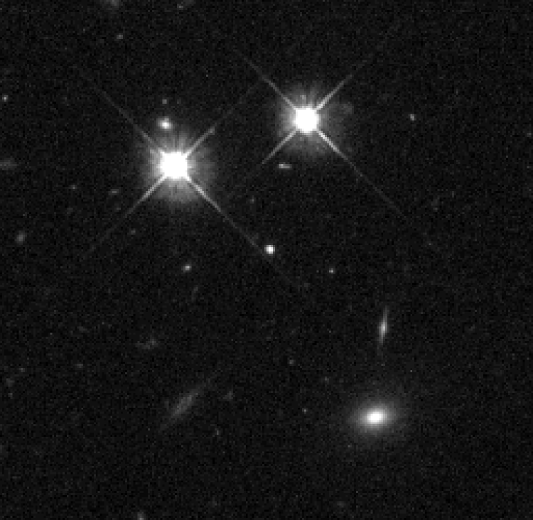
Figure 3: The original image, taken from the Space Telescope web page www.stsci.edu. It is the 100,000th image taken with HST for C. Steidel of Caltech.

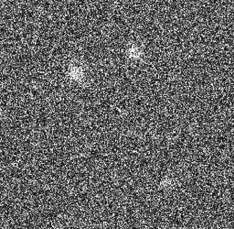
Figure 4: Figure 3 with substantial noise added.

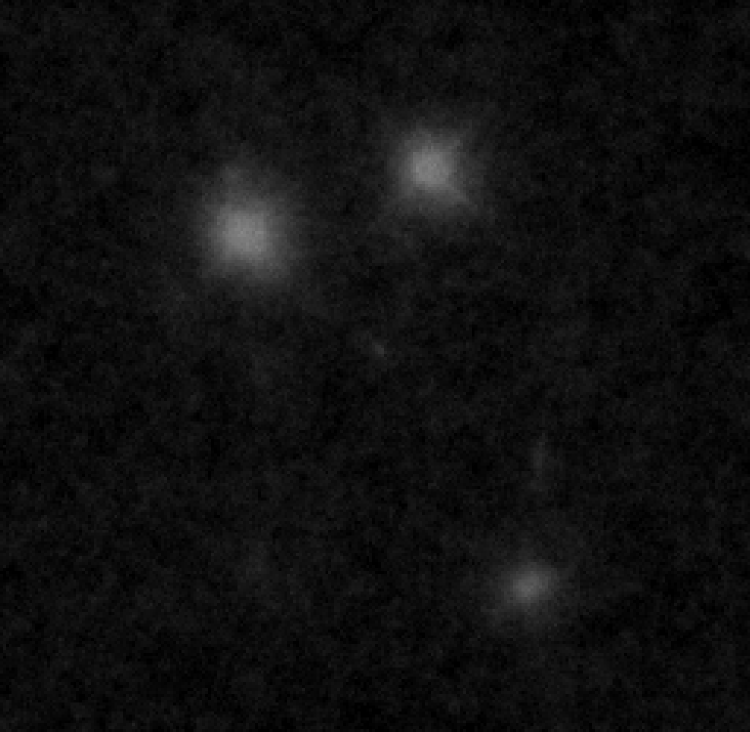
Figure 5: Wiener filtered. We see that the linear scaling function substantially reduces the flux in the bright stars.

We first apply a Wiener filter, with the result shown in figure 5. We notice immediately the key feature: all amplitudes are scaled by the noise, so the bright stars have been down scaled significantly. The noise on the star was less than unity, but each Fourier mode gets contributions from the star as well as the global noise of the image. The situation worsens if the filling factor of the signal regions is small. The mean intensity of the image is stored in the $k=0$ mode, which is not significantly affected by noise. While total flux is approximately conserved, the flux on each of the objects is non-locally scattered over the whole image by the Wiener filter process.

Figure 6: Non-Gaussian wavelet filtered. Several of the features that had been lost in the Wiener filtering process are recovered here.

The optimal Bayesian wavelet filter is shown in figure 6. A Daubechies 12 wavelet was used, and the prior PDF reconstructed using the scaling assumption described in section 3. We see immediately that the amplitudes on the bright objects are much more accurate. We see also that the faint vertical edge-on spiral on the lower right just above the bright elliptical is clearly visible in this image, while it had almost disappeared in the Wiener filter.

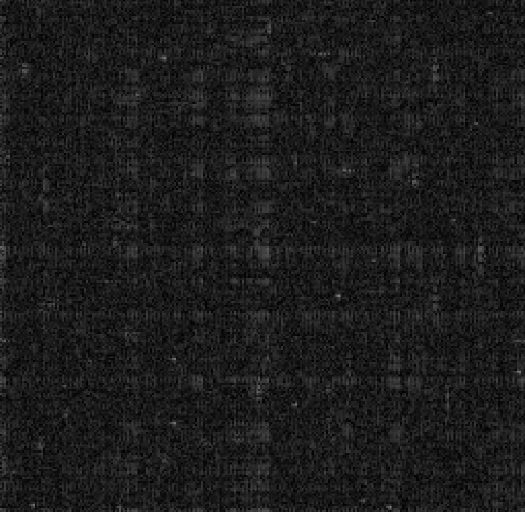
Figure 7: Error map. Plotted is the posterior Bayesian variance. We see that some features, for example the small dot in the upper left, have large errors associated with them, and are therefore artefacts.

The Bayesian approach allows us to estimate the error in the reconstruction using Equation (2). We show the result in figure 7. We can immediately see that some features in the reconstructed map, for example the second faint dot above the bright star on the upper left, have large errors associated with them, and are indeed artefacts of reconstruction. Additionally, certain wavelets experience large random errors. These appear as checkered ’wavelet’ patterns on both the reconstructed image and the error map.

5 Discussion

Fourier space has the advantage that for translation invariant processes, different modes are pairwise uncorrelated. If modes were truly independent, the optimal filter for each $k$ mode would also be globally optimal. As we have seen from the example in section 33.2, processes which are local in real space are not optimally processed in Fourier space, since different Fourier modes are not independent. Wavelet modes are not independent, either. For typical data, the correlations are relatively sparse. In the astronomical images under consideration, the stars and galaxies are relatively uncorrelated with each other. Wavelets with compact support sample a limited region in space, and wavelets which do not overlap on the same objects on the grid will be close to independent. Even for Gaussian random fields, wavelets are close to optimal since they are relatively local in Fourier space. Their overlap in Fourier space leads to residual correlations which are neglected. We see that wavelets are typically close to optimal, even though they are never truly optimal. But in the absence of a full prior, they allow us to work with generic data sets and usually outperform Wiener filtering.

In our analysis, we have used Cartesian product Daubechies wavelets. These are preferentially aligned along the grid axes. In the wavelet filtered map (figure 6) we see residuals aligned with the coordinate axes. Recent work by Kingsbury (this proceedings) using complex wavelets would probably alleviate this problem. The complex wavelets have a factor of two redundancy, which is used in part to sample spatial translations and rotational directions more homogeneously and isotropically.

6 Conclusions

We have presented a generalized noise filtering algorithm. Using the Ansatz that the PDF of mode or pixel coefficients is scale invariant, we can use the observed data set to estimate the PDF. By application of Bayes’ theorem, we reconstruct the filter map and noise map. The noise map gives us an estimate of the error, which tells us the performance of the particular basis used and the confidence level of each reconstructed feature. Based on comparison with controlled data, we find that the error estimates typically overestimate the true error by about a factor of two.

We argued that wavelet bases are advantageous for data with a small duty cycle that is localized in real space. This covers a large class of astronomical images, and images where the salient information is intermittently present.

- [1] Cornwell, T. & Braun, R. 1989, “Deconvolution”, in Synthesis Imaging in Radio Astronomy (Eds. R.A. Perley, F.R Schwab & A.H. Bridle), pp. 167-184.
- [2] Damiani, F., Maggio, A., Micela, G. & Sciortino, S. 1997a, “A Method Based on Wavelet Transforms for Source Detection in Photon-Counting Detector Images. I. Theory and General Properties”, Astroph. J., 483, 350-369.
- [3] Damiani, F., Maggio, A., Micela, G. & Sciortino, S. 1997b, “A Method Based on Wavelet Transforms for Source Detection in Photon-Counting Detector Images. II. Application to ROSAT PSPC Images”, Astroph. J., 483, 370-389.
- [4] Field, D. 1999, this proceedings.
- [5] Hobson, M.P., Joens, A.W. & Lasenby, A.N. 1998, “Wavelet Analysis and the Detection of non-Gaussianity in the CMB”, submitted to Mon. Not. Royal Astr. Soc, astro-ph/9810200.
- [6] Kingsbury, N. 1999, this proceedings.
- [7] Meyer, Y. 1992, Wavelets and Operators, ch 3.3, p 81, Cambridge University Press.
- [8] Pando, J. & Fang, L.-Z. 1996, “A Wavelet Space-Scale Decomposition Analysis of Structures and Evolution of QSO Ly Absorption Lines”, Astroph. J., 459, 1-11.
- [9] Press, W.H., Teukolski, S.A., Vetterling, W.T. & Flannery, B.P. 1992, Numerical Recipes, ch. 13-10, pp. 584-599, Cambridge University Press.
- [10] Slezak, E., Duret, F. & Gerbal, D. 1994, “A Wavelet Analysis Search for substructure in 11 X-ray Clusters of Galaxies”, Astrophys. J., 108, 1996-.
- [11] Silvermann, B. 1999, this proceedings.
- [12] Tenorio, L., Jaffe, A.H., Hanany, S. & Lineweaver, C.H. 1999, “Application of Wavelets to the Analysis of Cosmic Microwave Background Maps”, submitted to Mon. Not. Royal Astr. Soc., astro-ph/9903206.
- [13] Vidakovic, B. 1998, “Wavelet-Based Nonparametric Bayes Method”, in Practical Nonparametric and Semiparametric Baysian Statistics (Eds. Dey, Müller & Sinka), Springer-Verlad, LNS 133, 133-155.
- [14] Vogeley, M.S. & Szalay, A.S. 1996, “Eigenmode Analysis of Galaxy Redshift Surveys. I. Theory and Methods”, Astrophys. J., 465, 34-53.