Probing neutrino decays with the cosmic microwave background

Abstract

We investigate in detail the possibility of constraining neutrino decays with data from the cosmic microwave background radiation (CMBR). Two generic decays are considered $\nu_{H}\to\nu_{L}\phi$ and $\nu_{H}\to\nu_{L}\bar{\nu}_{L}\nu_{L}$. We have solved the momentum dependent Boltzmann equation in order to account for possible relativistic decays. Doing this we estimate that any neutrino with mass $m\gtrsim 1$ eV decaying before the present should be detectable with future CMBR data. Combining this result with other results on stable neutrinos, any neutrino mass of the order 1 eV should be detectable.

]

I introduction

The possibility that one or more neutrino species are unstable on a cosmologically interesting timescale has been considered very extensively in the literature (see for instance [1, 2, 3, 4, 5, 6, 7, 8, 9, 10, 11] and references therein). In particular it has been pointed out that cosmology is an excellent laboratory for neutrino physics and that many exotic neutrino models that are inaccessible to tests in terrestrial experiments may be tested using cosmology.

Big Bang nucleosynthesis has turned out to be a very powerful probe for this purpose [3, 4, 5, 6, 7, 8, 9, 10, 11]. However, one shortcoming of BBN in this regard is that it is only sensitive to physics before the end of nucleosynthesis, at $t\simeq 10^{3}$ s. After this the relative abundances of light elements is fixed until the present.

Another intriguing possibility is to use the CMBR to probe exotic neutrino physics [12, 13, 14, 15]. This has been done in the past to constrain neutrino decays and other effects of non-standard neutrinos. However, there has been no real coherent treatment of what limits can be put on neutrino decays from CMBR data. In the present work we shall try to discuss all the possible decay modes of a heavy neutrino in the context of CMBR.

II neutrino decays

A massive neutrino can in principle have many different decay modes. The simplest possibilities are the standard model decays $\nu_{H}\to\nu_{L}\gamma$ and $\nu_{H}\to e^{+}e^{-}\nu_{e}$ [16, 17]. However, they both suffer from the fact that their decay products contain electromagnetically interacting particles and they can therefore be observationally constrained. Raffelt [18] provides an excellent review on the observational limits on such decays. The main conclusion is that they are excluded unless the lifetime is exceedingly long.

We are then left with other possibilities which demand more exotic models. We shall look at two decay modes which cover the viable possibilities $\nu_{H}\to\nu_{L}\phi$ and $\nu_{H}\to\nu_{L}\bar{\nu}_{L}\nu_{L}$ [16, 17]. Below we shall discuss the possible scenarios where such decays can take place.

A $\nu_{H}\to\nu_{L}\phi$

The primary model for this type of decay is the majoron model [16]. This is a specific model for the generation of neutrino mass. In this model, the neutrino is a Majorana particle and $\phi$ is a scalar or pseudoscalar. If we assume a Yukawa type interaction of the form

$${\cal L}=g\phi\bar{\nu}_{L}\gamma_{5}\nu_{H}$$ (1)

and that the daughter particles are massless we obtain a rest-frame decay rate of

$$\Gamma=\frac{g^{2}m_{H}}{8\pi}.$$ (2)

It is possible to constrain $g$ from data on neutrinoless double beta decays to be $g\lesssim 10^{-4}$ [17]. Inserting numbers we get a lower bound to the lifetime of

$$\tau\gtrsim 1.6\times 10^{-12}\,m^{-1}_{\rm MeV}\,{\rm s}.$$ (3)

This bound is obviously not very restrictive and by far the best bounds on such decays come from astrophysical considerations.

B $\nu_{H}\to\nu_{L}\bar{\nu}_{L}\nu_{L}$

This decay is somewhat more complicated. However, three-body decays are an equally interesting possibility which arises in left-right symmetric models and in general in models with neutral current flavour violation. A neutrino decay will then be mediated by either a Higgs, $\Delta_{0}$, or a $Z^{\prime}$ [16]. In either case, it is safe to assume that the boson exchanged is extremely heavy so that the decay is effectively a four-point interaction.

An interesting question is how fast such three-body decays can proceed in realistic models. If one assumes a non-derivative coupling as would be the case for both the above possibilities then one arrives at an amplitude of

$$M=\frac{G}{\sqrt{2}}\bar{u}_{2}Ou_{1}\bar{u}_{4}Ov_{3},$$ (4)

where the coupling $O$ is given by

$$O=\{I,\gamma_{5},\gamma_{\mu},\gamma_{\mu}\gamma_{5}\},$$ (5)

or a combination of these operators.

Since all of the final-state particles are identical (assuming that there is $CP$ symmetry), all of these different possibilities give the same decay kinematics because of the indistinguishability of the final state particles, the only difference being the absolute decay rate. This of course simplifies the calculations a lot. We need do only one calculation for each value of the rest frame decay rate, $\Gamma$. This quantity is directly related to the coupling strength $G$ by

$$\frac{1}{\tau}=\Gamma=CG^{2}\frac{m^{5}}{\pi^{3}},$$ (6)

where $C$ is a constant which depends on the specific form of the operator $O$. In the remainder of the paper we shall refer to the matrix element for this process as a “weak” matrix element because it arises from interactions very similar in structure to the standard weak interactions.

For comparison we also calculate how three-body decays proceed if the decay matrix element is constant

$$\sum|M|^{2}=K=G^{2}m^{4}.$$ (7)

This gives a rest frame-decay lifetime of

$$\frac{1}{\tau}=\Gamma=\frac{m^{5}}{512\pi^{3}}G^{2}.$$ (8)

To see what lifetimes can be expected in such a model we take an example where the decay is through a flavour violating neutral current. We can rewrite the coupling constant as $G^{2}=\theta^{2}G_{F}^{2}$ and from this we get

$$\tau=2.88\times 10^{14}\,\theta^{2}m_{\rm MeV}^{-5}\,{\rm s}.$$ (9)

The limit on $\theta$ is of the order $\theta\lesssim 10^{-5}$ [16] which means that for $m\lesssim 0.2$ MeV, the decay lifetime is longer than the Hubble time.

Of course one might postulate a fast invisible decay mode to a three neutrino final state, and its effect on cosmology would then be one way of detecting it. For this reason alone it is interesting to calculate thoroughly how such a decay would affect cosmology. In the following we shall just take a heuristic approach and examine the consequences of a fast three-body decay without looking at the theoretical background for this.

III formalism

In the following we will go through the formalism needed to calculate decay rates and distributions for both two- and three-body decays. In general we need to solve the Boltzmann equation which has the form [19]

$$L[f]=C_{D}[f],$$ (10)

where

$$L[f]=\frac{\partial f}{\partial t}-Hp\frac{\partial f}{\partial p}.$$ (11)

The right hand side of the equation describes decay terms of various sort. These are quite different for two and three body decays and we shall discuss each in turn.

A two body decays

Two body decays have quite simple kinematics since the rest-frame energy of each daughter particle is well defined and equal to $m_{H}/2$. We get for the decay terms [20]

$$C_{\mbox{{dec}}}[f_{\nu_{H}}]=-\frac{m_{\nu_{H}}^{2}}{\tau m_{0}E_{\nu_{H}}p_{\nu_{H}}}\int_{E_{\phi}^{-}}^{{E_{\phi}^{+}}}dE_{\phi}\Lambda(f_{\nu_{H}},f_{\nu_{L}},f_{\phi})$$ (12)

$$C_{\mbox{{dec}}}[f_{\nu_{L}}]=\frac{g_{\nu_{H}}}{g_{\nu_{L}}}\frac{m_{\nu_{H}}^{2}}{\tau m_{0}E_{\nu_{L}}p_{\nu_{L}}}\int_{E_{\nu_{H}}^{-}}^{{E_{\nu_{H}}^{+}}}dE_{\nu_{H}}\Lambda(f_{\nu_{H}},f_{\nu_{L}},f_{\phi})$$ (13)

$$C_{\mbox{{dec}}}[f_{\phi}]=\frac{g_{\nu_{H}}}{g_{\phi}}\frac{m_{\nu_{H}}^{2}}{\tau m_{0}E_{\phi}p_{\phi}}\int_{E_{\nu_{H}}^{-}}^{{E_{\nu_{H}}^{+}}}dE_{\nu_{H}}\Lambda(f_{\nu_{H}},f_{\nu_{L}},f_{\phi}),$$ (14)

where $\Lambda(f_{\nu_{H}},f_{\nu_{L}},f_{\phi})=f_{\nu_{H}}(1-f_{\nu_{L}})(1+f_{\phi})-f_{\nu_{L}}f_{\phi}(1-f_{\nu_{H}})$, $m_{0}^{2}=m_{\nu_{H}}^{2}-2(m_{\phi}^{2}+m_{\nu_{L}}^{2})+(m_{\phi}^{2}-m_{\nu_{L}}^{2})^{2}/m_{\nu_{H}}^{2}$. $\tau$ is the lifetime of the heavy neutrino and $g$ is the statistical weight of a given particle. We use $g_{\nu_{H}}=g_{\nu_{L}}=2$ and $g_{\phi}=1$, corresponding to $\phi=\overline{\phi}$ The integration limits are

$$E_{\nu_{H}}^{\pm}(E_{i}) = \frac{m_{0}m_{\nu_{H}}}{2m_{i}^{2}}[E_{i}(1+4(m_{i}/m_{0})^{2})^{1/2}\pm$$ (16)

$$(E_{i}^{2}-m_{i}^{2})^{1/2}]$$

and

$$E_{i}^{\pm}(E_{\nu_{H}})=\frac{m_{0}}{2m_{\nu_{H}}}[E_{\nu_{H}}(1+4(m_{i}/m_{0})^{2})^{1/2}\pm p_{\nu_{H}}]$$ (17)

where the index $i=F,\phi$.

B three body decays

The decay term in the Boltzmann equation can in this case be written as [19, 21]

$$C_{\text{D}}[f] = \frac{1}{2E_{1}}\int d^{3}\tilde{p}_{2}d^{3}\tilde{p}_{3}d^{3}\tilde{p}_{4}\Lambda(f_{1},f_{2},f_{3},f_{4})$$ (19)

$$\,\,\,\times\sum|M|^{2}\delta^{4}({\it p}_{1}+{\it p}_{2}-{\it p}_{3}-{\it p}_{4})(2\pi)^{4},$$

with $d^{3}\tilde{p}_{i}=d^{3}p_{i}/(2E_{i}(2\pi)^{3})$ and $\Lambda(f_{1},f_{2},f_{3},f_{4})=(f_{2}f_{3}f_{4}(1-f_{1})-f_{1}(1-f_{2})(1-f_{3})(1-f_{4}))$. Details of how to evaluate this phase-space integral can for instance be found in Ref. [22].

The simplest frame to evaluate the phase space integral in is the rest frame of the parent particle. Since the three body decay scheme does not yield a specific energy for the daughter particles, it is interesting to study how the energy distribution of daughter particles differ for the different interaction matrix elements. In order to do this it is very convenient to calculate the differential production rate of daughter particles

$$\frac{d\Gamma}{dp}=\Gamma_{0}\times\cases{8p/m&constant,\cr 64(p/m)^{2}(1-\frac{5}{3}p/m)&``weak''.}$$ (20)

It should be noticed here that the maximum attainable momentum for any daughter particle is $m/2$ in order to have 4-momentum conservation. In Fig. 1 we have plotted the decay distributions for both cases. The most interesting feature is that the weak matrix element leads to a decay distribution which is stronger peaked in momentum space.

FIG. 1.: The differential energy distribution of the light neutrino for three different possibilities. The full line is from the “weak” matrix element, the dotted for the constant matrix element and the dashed for the standard model decay $\nu_{H}\to\nu_{L}e^{+}e^{-}$. The lines have been normalised to $\Gamma=1$.

In the standard model decay $\nu_{H}\to\nu_{L}e^{+}e^{-}$ one gets instead the “standard” result for the decay distribution of the neutrino [7]

$$\frac{d\Gamma}{dp}=\Gamma_{0}\times 48(p/m)^{2}(1-\frac{4}{3}p/m).$$ (21)

The reason why our result is different is that we assume that all three final state particles are identical. As for the average energy of the emitted neutrinos, it is of course equal to $m/3$ both for the both types of matrix elements. For the standard model decay above, it is equal to $7m/20$, which is slightly higher.

C background cosmology

In order to get the decay into a proper cosmological setting it is then necessary to prescribe how the universe in general evolves with time. In the simple case where the universe is radiation dominated at decay and the energy densities of both parent and daughters is subdominant, the time-temperature relation is simply [21]

$$t(s)=1.71\,g_{*}^{-1/2}T_{\rm MeV}^{-2},$$ (22)

where $g_{*}$ is the effective number of degrees of freedom. However, in general this is not true because the decay might take place while the universe is matter dominated or partly matter dominated. In this more general case it is necessary to use the equation of energy conservation

$$\frac{d}{dt}(\rho R^{3})+p\frac{d}{dt}(R^{3})=0,$$ (23)

which is an exact equation, together with the Friedmann equation

$$H^{2}=\frac{8\pi G\rho}{3}-\frac{k}{R^{2}},$$ (24)

in order to get a relation between time and temperature in the universe [21].

IV numerical solution of the Boltzmann equation

In order to investigate the impact on the CMBR of decays it is necessary solve the Boltzmann equation numerically. To do this we have used a grid in comoving momentum space.

However, first we have to determine the initial conditions of the system. Primarily this means that we must discuss whether or not the daughter particles have thermal distributions prior to decay. For the $\phi$-particle we shall assume that it is not present prior to decay. This will be the case if the particle decoupled from thermal equilibrium prior to the QCD phase-transition [21]. For the light neutrino there are two possibilities, either $\nu_{L}$ is one of the three active species or it is a sterile species. In the former case we assume a thermal distribution prior to decay and in the latter we assume that there are no light neutrinos present before the decay commences. We shall always assume that the parent neutrino has a thermal population prior to decay.

For a qualitative discussion of the decays it is convenient to introduce a relativity parameter $\alpha$ for the decay [10]. Here, we assume that the universe is radiation dominated during the decay. A species becomes non-relativistic roughly when $T=m/3$. Using this the relativity parameter can be written as

$$\alpha\equiv 6.5\times 10^{-2}g_{*}^{1/2}\tau_{\rm s}m_{\rm MeV}^{2}.$$ (25)

The decay is then relativistic if $\alpha\lesssim 1$ and non-relativistic if $\alpha\gtrsim 1$.

Here we have used the simple relation, Eq. (22). This has been done in order to make the decay physics more transparent, but in the next section where actual mass-lifetime limits are calculated we use the energy conservation and Friedmann equations, Eqs. (23-24).

FIG. 2.: The final energy density in decay products for the different possible decays, parametrised in equivalent neutrino species. The standard model with no decay would correspond to $N_{\nu,{\rm eff}}=1$.

A two body decays

The two-body decay is interesting in that one of the final state particles is a boson. This means that because of stimulated emission effects there will be a large population of low momentum $\phi$’s. This of course only happens if these states are accessible, i.e. for relativistic decays [6, 20] In the Appendix we have calculated the final energy density in decay products for both very relativistic and completely non-relativistic decays. These results are compared with the full Boltzmann solution in Fig. 2. The full solution clearly has the correct asymptotic behaviour.

B three body decays

For non-relativistic decays, the cosmic frame is equal to the rest-frame of the parent particle. In this case, for equal total decay rates, the “weak” and the constant matrix element give somewhat different decay distributions. The reason is that energy and number conservation only yields two fixed parameters. For an equilibrium distribution this is sufficient to describe the distribution fully by a temperature and a pseudo-chemical potential, but the distribution of the daughter particle is not an equilibrium one so that there are no two parameters fully describing the distribution function.

For extremely relativistic decays the decay and inverse decay installs equilibrium in the particle distributions for both parent and daughter. In this case, the decay proceeds in complete equilibrium and the final distribution functions become identical, independent of the actual matrix element.

We have plotted the final momentum distribution of the daughter particles for different values of the relativity parameter, $\alpha$. Indeed one sees that for very relativistic decays the distributions become identical. For non-relativistic decays they become very significantly different, even though the zeroth and first moments are identical. If one is interested in applications where the actual shape of the distribution is important, as would be the case if the daughter is an electron neutrino present during nucleosynthesis [10, 11] or an eV particle constituting the Hot Dark Matter [23], this difference in distribution could potentially be important. However, if one is interested only in the final number and energy density, the difference between using different matrix elements is indeed very small and can be safely ignored.

It is quite interesting to compare the final decay distributions with equilibrium distributions of the form

$$f_{\rm eq}(p)=\frac{1}{\exp\left(\frac{p-\mu}{T}\right)+1},$$ (26)

with the same number and energy densities as the true distributions. We have plotted these equilibrium distributions together with the full distributions calculated from the Boltzmann equation in Fig. 3. It is seen that in the strongly relativistic case the decay proceeds in equilibrium and the final distributions are of equilibrium form. For strongly non-relativistic decays the equilibrium distributions are quite poor approximations to the true distribution functions, as expected.

FIG. 3.: The final momentum distribution of the light neutrino after decay for the three body decay $\nu_{H}\to\nu_{L}\bar{\nu}_{L}\nu_{L}$. The full line is for the “weak” matrix element, the dotted for the constant matrix element and the dashed line shows an equilibrium distribution with the same number and energy density. The five sets of curves correspond from left to right to $\alpha$ = 0.2, 2, 10, 100, 500.

V CMBR effects

Using the results on the energy density evolution of the decaying particle and its daughters we can now proceed to investigate the CMBR effects from neutrino decays. The fluctuations are usually described in terms of spherical harmonics [24]

$$T(\theta,\phi)=\sum_{lm}a_{lm}Y_{lm}(\theta,\phi),$$ (27)

where the coefficients are related to $C_{l}$ coefficients by

$$C_{l}\equiv\langle|a_{lm}|^{2}\rangle.$$ (28)

These fluctuations were first detected in 1992 by the COBE satellite [25], but only for $l\lesssim 20$. At such low $l$ the power spectrum is almost degenerate in the cosmological parameters and no real constraints are obtainable. In the next few years, however, the power spectrum will hopefully be measured out to $l\simeq 2500$ by two new probes, MAP and PLANCK [26], and using this data should yield precision measurements of the physical parameters at recombination. We shall here assume that MAP will deliver data out to $l=1000$ and PLANCK to $l=2500$.

Since we do not yet have the precision data in hand it is hard to foretell how accurately the different parameters can actually be measured. The usual procedure is to use what is called error forecasting [27]. This method assumes an underlying cosmological model to be the “true” model. From that one can calculate how sensitive the data are to changes in the cosmological parameters. It should be noted here that this method can at best give an estimate of the obtainable precision. Once the data becomes available the actual problem of determining the cosmological parameters will be much tougher because the whole parameter space has to be investigated.

In the present paper we shall assume as the reference the standard cold dark matter model which can be described by a vector of values in the many-dimensional parameter space [27]

$$\Theta=(\Omega,\Omega_{b},\Lambda,h,n,\tau).$$ (29)

As free parameters we have chosen the total density, $\Omega$, the density in baryons, $\Omega_{b}$, the cosmological constant, $\Lambda$, the Hubble parameter, $h$, the spectral index, $n$, and the optical depth to reionisation, $\tau$. In addition to this we have included as free parameters the energy density injected by neutrino decays as well as the time at which the energy is injected.

Our choice of reference model is “standard” cold dark matter

$$\Theta_{\rm CDM}=(1,0.08,0,0.5,1,0).$$ (30)

Note that we have chosen a limited set of free parameters. In principle one should use a parameter space consisting of all possible free parameters.

Our procedure will then be the following: for given lifetime $\tau_{H}$ of the heavy neutrino we calculate which mass range will be detectable by the upcoming CMBR experiments. To estimate the obtainable precision we use the Fisher information matrix [27]

$$I_{ij}=\sum_{l=2}^{l_{\rm max}}(2l+1)\left[C_{l}+C_{l,{\rm error}}\right]^{-2}\frac{\partial C_{l}}{\partial\theta_{i}}\frac{\partial C_{l}}{\partial\theta_{j}},$$ (31)

where $C_{l,{\rm error}}$ represents the experimental error which we neglect in the present paper. The standard error in parameter $i$ is then

$$\sigma_{i}^{2}\simeq(I^{-1})_{ii},$$ (32)

if all cosmological parameters must be determined simultaneously, and

$$\sigma_{i}^{2}\simeq(I_{ii})^{-1},$$ (33)

if all the other parameters are assumed to have already been determined [12]. To calculate actual CMBR spectra we use the CMBFAST package designed by Seljak and Zaldarriaga [28].

To be on the conservative side we have calculated the sensitivity of the CMBR for the case where all parameters must be determined simultaneously. The results are shown in Fig. 4 where the upper panel shows the expected accuracy of PLANCK and the lower panel that of MAP. For very small neutrino masses the the decay cannot take place before $t(m/3)$. Also, the CMBR data are less sensitive to late decays. Therefore there is a sharp and well defined minimum mass which is detectable through CMBR measurements. This lower limit depends on the decay mode because the energy deposited in relativistic particles depends on the specific decay kinematics.

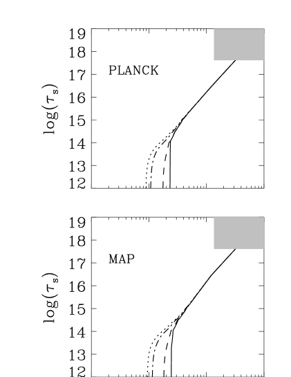
FIG. 4.: The expected detectable neutrino mass and lifetime with new CMBR data. The region to the right of the curves is the detectable range. Curve labels are as in Fig. 2. The shaded regions in both plots correspond to the detectable range found by Hu, Eisenstein and Tegmark [29].

For both early and late decays the main effect on CMBR is through the ISW effect [27]. This effect is due to the fact that if the universe has a significant radiation content the linear gravitational potential is not constant in time. This leads to an enhancement of the CMBR fluctuations, primarily on the scale corresponding to the horison size when the energy is injected.

Our results may be combined with the results of Hu, Eisenstein and Tegmark [29] on stable low mass neutrinos. They estimate that for stable neutrinos a combination of large scale structure surveys and CMBR measurements should be able to measure a neutrino mass of 1-2 eV.

Our estimate of the obtainable precision is clearly much more restrictive than that found by Lopez et al. [13], because they rely only on already existing CMBR data, which is of low accuracy. What we have shown is that the CMBR is a very sensitive probe of neutrino decays. Clearly, our limits only apply to the case where decay takes place after neutrinos have decoupled completely from thermal equilibrium at $T\simeq 0.1$ MeV.

VI Discussion

In this paper we have calculated the constraints that it should be possible to put on neutrino decays using data from the new CMBR experiments. We have paid particular attention to the different possible decay modes, discussing both two- and three-body decays in detail. Also, the full Boltzmann equation was solved, instead of the momentum integrated version [21]. This has the clear advantage that it is possible to do calculations for relativistic neutrino decays where inverse decays are included.

Using this formalism we estimated that it should be possible to constrain any type of neutrino decay if the mass is of the order 1-2 eV. If the lifetime is short it may be possible to detect neutrino masses down to 0.1 eV using this method. Our results complement and extend existing results on CMBR constraints on neutrino decays [13, 14]

Finally, it is of interest to discuss how a decaying neutrino scenario relates to the recent results from Super-Kamiokande. According to these results the muon neutrino oscillates with near maximum mixing with another neutrino, most likely the tau neutrino [30]. The mass difference between these two states is of the order 0.1 eV, and if one simultaneously believes the solar neutrino anomaly to be due to $\nu_{e}-\nu_{\mu}$ oscillations [31] there is no room left for cosmologically interesting neutrino decays. However, there might be other possibilities. For instance the solar neutrino solution might be due to oscillations with a sterile neutrino state. The only constraint is then that $\nu_{\mu}$ and $\nu_{\tau}$ should be almost degenerate in mass. This could still allow for cosmologically interesting and detectable decays. Until there are more firm results on this subject, neutrino decays remain a viable possibility.

A Asymptotic behaviour

1 decay in equilibrium

If the decay is relativistic it is a very good approximation to assume that it proceeds in equilibrium. This means that the distribution functions are all of equilibrium form

$$f_{{\rm eq},i}(E)=\frac{1}{\exp\left(\frac{E-\mu_{i}}{T_{i}}\right)+1}.$$ (A1)

In this case, instead of using the Boltzmann equation, we can derive a very simple set of equations for the temperature and pseudo-chemical potentials.

The procedure is the following: One starts at some initial time with given initial conditions. Then at each timestep the distributions are evolved forwards in time and then allowed to equilibrate completely before the next timestep is taken.

We start with the two-body decay. In this case the equations to be solved at each timestep are

$$\mu_{H} = \mu_{L}$$ (A2)

$$n_{0} = n_{H}+n_{L}$$ (A3)

$$\rho_{0} = \rho_{H}+\rho_{L}+\rho_{\phi}$$ (A4)

$$n_{L} = n_{\phi}.$$ (A5)

$$T_{H} = T_{L}=T_{\phi}$$ (A6)

An interesting possibility in this case is that it is possible to form a Bose-condensate from the pseudo-scalar particle. This phenomenon has been investigated previously in the literature [6]

For the three body decay, the corresponding equations are

$$\mu_{H} = 3\mu_{L}$$ (A7)

$$n_{0} = n_{H}+n_{L}/3$$ (A8)

$$\rho_{0} = \rho_{H}+\rho_{L}$$ (A9)

$$T_{H} = T_{L}.$$ (A10)

We have solved these equations to obtain the final energy density in the daughter products since this is the relevant quantity to know if we are interested in effects on the CMBR.

It is of course also worth noting that for relativistic decays there is no entropy production since all the distribution functions stay in kinetic equilibrium throughout [19]. Also, the final energy density in decay products is completely independent of the expansion rate of the universe since equilibration is assumed to happen instantaneously at each temperature. In Table I we have shown the final energy density for relativistic decays for the four different possibilities which we have treated.

TABLE I.: Final energy density in the decay products in units of a massless neutrino species.

Decay	$N_{\nu_{L},0}$	$N_{\nu,{\rm eff}}$
$\nu_{H}\to\nu_{L}\phi$	0	$1.20$
$\nu_{H}\to\nu_{L}\phi$	thermal	$1.48$
$\nu_{H}\to\nu_{L}\bar{\nu}_{L}\nu_{L}$	0	$2.20$
$\nu_{H}\to\nu_{L}\bar{\nu}_{L}\nu_{L}$	thermal	$2.63$

2 non-relativistic decays

For strongly non-relativistic decays the behaviour is also quite simple. Since the energy in the decaying particle is equal to the mass, $m$, we can write an equation for the evolution of energy density in decay products

$$\frac{\rho}{\rho_{0}}=\int_{t_{i}}^{t}\frac{e^{-t/\tau}}{\tau}\frac{m}{\langle E_{0}\rangle}dt,$$ (A11)

where $\rho_{0}$ is the energy density in a standard massless species. $\langle E_{0}\rangle=3.151\,T$ is the mean energy of a massless fermion and $t_{i}$ is some initial time which is taken to be $t_{i}\ll\tau$. Solving this equation we get

$$\frac{\rho}{\rho_{0}}=\frac{270\,\zeta(3)}{7\,\pi^{7/2}}\alpha^{1/2}\simeq 0.84\,\alpha^{1/2},$$ (A12)

for decays in the radiation dominated era and

$$\frac{\rho}{\rho_{0}}=\frac{540\,\zeta(3)}{7\,\pi^{4}}\Gamma\left(\frac{5}{3}\right)\alpha^{2/3}\simeq 0.86\,\alpha^{2/3},$$ (A13)

for decays in the matter dominated regime.

REFERENCES

- [1] S. Bharadwaj and S. K. Sethi, Astrophys. J. Suppl. 114, 37 (1998).
- [2] M. White, G. Gelmini and J. Silk, Phys. Rev. D 54, 1301 (1006).
- [3] N. Terasawa and K. Sato, Phys. Lett. B 185, 412 (1987).
- [4] E. W. Kolb and R. J. Scherrer, Phys. Rev. D 25, 1481 (1982).
- [5] R. J. Scherrer and M. S. Turner, Astrophys. J. 331, 19 (1988); R. J. Scherrer and M. S. Turner ibid. 331, 31 (1988).
- [6] J. Madsen, Phys. Rev. Lett. 69, 571 (1992).
- [7] S. Dodelson, G. Gyuk and M.S. Turner, Phys. Rev. D 49, 5068 (1994).
- [8] M. Kawasaki et al., Nucl. Phys. B419, 105 (1994).
- [9] M. Kawasaki, K. Kohri and K. Sato, Report no. astro-ph/9705148.
- [10] S. Hannestad, Phys. Rev. D 57, 2213 (1998).
- [11] A. D. Dolgov, S. H. Hansen and S. Pastor, hep-ph/9809598 (1998).
- [12] R. E. Lopez et al., astro-ph/9803095 (1998).
- [13] R. E. Lopez et al., Phys. Rev. Lett. 81, 3075 (1998).
- [14] S. Hannestad, Phys. Lett. B431, 363 (1998).
- [15] S. Hannestad and G. Raffelt, Phys. Rev. D 59, 043001 (1999).
- [16] R. N. Mohapatra and P. B. Pal, Massive Neutrinos in Physics and Astrophysics, World Scientific Lecture Notes in Physics - Vol. 41, World Scientific 1991.
- [17] C. W. Kim and A. Pevsner, Neutrinos in Physics and Astrophysics, Harwood Academic Publishers (1993).
- [18] G. G. Raffelt, Stars as Laboratories for Fundamental Physics, University of Chicago Press (1996).
- [19] J. Bernstein, Kinetic Theory in the Expanding Universe, Cambridge University Press (1988).
- [20] G. D. Starkman, N. Kaiser, and R. A. Malaney, Astrophys. J. 434, 12 (1994).
- [21] E. W. Kolb and M. S. Turner, The Early Universe, Addison Wesley (1990).
- [22] S. Hannestad and J. Madsen, Phys. Rev. D 52, 1764 (1995).
- [23] S. Hannestad, Phys. Rev. Lett. 80, 4621 (1998).
- [24] P. Coles and F. Lucchin, Cosmology - The origin and evolution of cosmic structure, John Wiley & Sons (1995).
- [25] G. F. Smoot et al., Astrophys. J. 396, L1 (1992).
-
[26]
For information on these missions see the internet
pages for MAP (http://map.gsfc.nasa.gov) and PLANCK
(http://astro.estec.esa.nl/Planck/). - [27] M. Tegmark, in Proc. Enrico Fermi Summer School, Course CXXXII, Varenna (1995).
- [28] U. Seljak and M. Zaldarriaga, Astrophys. J. 469, 437 (1996).
- [29] W. Hu, D. J. Eisenstein and M. Tegmark, Phys. Rev. Lett. 80, 5255 (1998).
- [30] Y. Fukuda et al., Phys. Rev. Lett. 81, 1562 (1998)
- [31] J. N. Bahcall, P. I. Krastev, and A. Yu. Smirnov, hep-ph/9807216 (1998).