The reheating and reionization history of the universe.

Abstract

We incorporate quasars into an analytic model to describe the reheating and reionization of the universe. In combination with a previous study of galaxies and Lyman-$\alpha$ clouds, we are able to provide a unified description of structure formation, verified against a large variety of observations. We also take into account the clumping of the baryonic gas in addition to the presence of collapsed objects.

We consider two cosmologies: a critical universe with a CDM power-spectrum and an open universe with $\Omega_{0}=0.3$, $\Lambda=0$. The derived quasar luminosity function agrees reasonably well with observations at $z<4.5$ and with constraints over larger redshifts from the HDF. The radiation produced by these objects at $z\sim 16$ slowly reheats the universe which gets suddenly reionized at $z_{ri}=6.8$ for the open universe ($z_{ri}=5.6$ for the critical density universe). The UV background radiation simultaneously increases sharply to reach a maximum of $J_{21}=0.18$ at $z=2.6$, but shows strong ionization edges until $z\leq 1$. The metallicity of the gas increases quickly at high $z$ and is already larger than $0.01Z_{\odot}$ at $z=10$. The QSO number counts and the helium opacity constrain the reionization redshift to be $z_{ri}\sim 6$. We confirm that a population of faint quasars is needed in order to satisfy the observations. Due to the low reionization redshift, the damping of CMB fluctuations is quite small, but future observations (e.g. with the NGST) of the multiplicity functions of radiation sources and of the HI and HeII opacities will strongly constrain scenarios in which reionization is due to QSOs. The reasonable agreement of our results with observations (for galaxies, quasars, Lyman-$\alpha$ clouds and reionization constraints) suggests that such a model should be fairly realistic.

1 Introduction

An important goal of cosmology is to describe the structure formation processes which led to the wide variety of astrophysical objects we observe in the present universe, from Lyman-$\alpha$ clouds to galaxies and clusters. Several studies have shown that the usual hierarchical scenarios (like the standard CDM model) can provide predictions which agree reasonably well with observations for galaxies as well as for Lyman-$\alpha$ clouds. This corresponds to objects at $z\leq 5$. However, it is possible to constrain the earlier evolution of the universe by studying the reheating and reionization history implied by such models. Indeed, observations show that the universe is highly photo-ionized by $z=5$ and a large reionization redshift could imprint a signature on the CMB radiation. Moreover, future missions such as NGST could for instance detect quasars at high redshifts $z>5$.

In this article, we present an analytic model for the reheating and reionization history of the universe, adopting a CDM power spectrum in a critical density and in an open universe. Similar studies have been performed previously via numerical simulations (e.g. Gnedin & Ostriker 1997) and analytic approaches (e.g. Haiman & Loeb 1997; Haiman & Loeb 1998) based on the Press-Schechter prescription (Press & Schechter 1974). However, previous analytic models were often developed for this specific purpose (i.e. they were not derived from a model already checked in detail against observations of galaxies or Lyman-$\alpha$ clouds) and neglected the clumping of the gas (except for the presence of virialized objects used to count galaxies). Thus, the main motivations of our present study are to:

- describe these early stages of structure formation through a self-consistent model which has already been applied to galaxies (Valageas & Schaeffer 1998) and to Lyman-$\alpha$ clouds (Valageas et al.1999a).

- take into account the broad range of density fluctuations within the IGM through our description of Lyman-$\alpha$ clouds.

- use this feature to constrain our model against several observations: notably the QSO number counts and the Gunn-Peterson test (for HI and HeII).

- develop a simple analytic model which can predict many properties of the universe (galaxy and quasar luminosity functions, temperature and ionization state of the IGM, intensity and spectrum of the UV background radiation and fraction of matter within stars) and provide a complementary tool to numerical simulations.

Consideration of the various objects involved in our work (beyond the just-virialized halos which are usually studied) is made possible because of a specific description of the density field based on the assumption that the many-body correlation functions obey the scaling model detailed in Balian & Schaeffer (1989) and checked numerically in Colombi et al.(1997). This allows one to define the various mass functions of interest, as described in Valageas & Schaeffer (1997; also in Valageas et al.1999b), and to go beyond the scope of the usual Press-Schechter approximation (Press & Schechter 1974). The main advantage of our approach is thus to provide a globally consistent picture of structure formation in the universe, within the framework of a hierarchical scenario.

This article is organized as follows. In Sect.2 we describe our prescription for mass functions. Next, in Sect.3 we review our model for galaxy formation, described in more detail in Valageas & Schaeffer (1998) while in Sect.4 we deal with our prescription for quasars. In Sect.5 we summarize the relevant aspects of our model for Lyman-$\alpha$ clouds (Valageas et al. 1999a). We describe the calculation of the evolution of the IGM properties (temperature, UV background radiation, ionization state) in Sect.6 and in Sect.7. Finally, in Sect.8 and Sect.9 we present our results for the case of an open universe and then for a critical universe.

2 Multiplicity functions

We first review the method we use to obtain the mass functions of various astrophysical objects, specifically galaxies and Lyman-$\alpha$ clouds. We consider objects of dark matter mass $M$ to be defined by a density threshold $\Delta(M,z)$. This constraint depends on the class of astrophysical objects one considers and it allows us for instance to distinguish clusters from galaxies which correspond to higher density contrasts (see VS II). Lyman-$\alpha$ clouds are also formed by several populations of different objects which are not always defined by a constant density threshold (see Sect.5). Note that such a goal is beyond the reach of the usual Press-Schechter prescription (Press & Schechter 1974) which only deals with “just-collapsed halos” while we wish to describe simultaneously a wide variety of objects. In any case, we attach to each halo a parameter $x$ defined by:

$$x(M,z)=\frac{1+\Delta(M,z)}{\;\overline{\xi}[R(M,z),z]\;}$$ (1)

where

$$\overline{\xi}(R)=\int_{V}\frac{d^{3}r_{1}\;d^{3}r_{2}}{V^{2}}\;\xi_{2}({\bf r}_{1},{\bf r}_{2})\;\;\;\;\;\mbox{with}\;\;\;\;\;V=\frac{4}{3}\pi R^{3}$$

is the average of the two-body correlation function $\xi_{2}({\bf r}_{1},{\bf r}_{2})$ over a spherical cell of radius $R$ and provides the measure of the density fluctuations in such a cell. Then, we write the multiplicity function of these objects (defined by the constraint $\Delta(M,z)$) as (see VS I):

$$\eta(M,z)\frac{dM}{M}=\frac{\overline{\rho}}{M}\;x^{2}H(x)\;\frac{dx}{x}$$ (2)

where $\overline{\rho}$ is the mean density of the universe at redshift $z$, while the mass fraction in halos of mass between $M$ and $M+dM$ is:

$$\mu(M,z)\frac{dM}{M}=x^{2}H(x)\;\frac{dx}{x}$$ (3)

The scaling function $H(x)$ depends only on the initial spectrum of the density fluctuations and must be obtained from numerical simulations. However, from theoretical arguments (see VS I and Balian & Schaeffer 1989) it is expected to follow the asymptotic behaviour:

$$x\ll 1\;:\;H(x)\propto x^{\omega-2}\hskip 8.5359pt,\hskip 8.5359ptx\gg 1\;:\;H(x)\propto x^{\omega_{s}-1}\;e^{-x/x_{*}}$$

with $\omega\simeq 0.5$, $\omega_{s}\sim-3/2$, $x_{*}\sim 10$ to 20 and by definition it must satisfy

$$\int_{0}^{\infty}x\;H(x)\;dx=1$$ (4)

The correlation function $\overline{\xi}$, that measures the non-linear fluctuations at scale $R$ can be modelled in a way that accurately follows the numerical simulation. The mass functions obtained from (2) for various constraints $\Delta(M)$ were checked against the results of numerical simulations in Valageas et al.(1999b) in the case of a critical universe with an initial power-spectrum which is a power-law: $P(k)\propto k^{n}$ with $n=0,-1$ and $-2$. This study showed that this model provides a reasonable approximation to the mass functions obtained in the simulations and that it works quite well for the two cases we shall need in the present article: i) a constant density threshold $\Delta\sim 178$ and ii) a constant radius constraint (or $(1+\Delta)\propto M$). Moreover, the results of Valageas et al.(1999b) showed that $H(x)$ is close to a similar scaling function $h(x)$ obtained from the counts-in-cells statistics, as expected from theoretical considerations (see for instance VS I).

It is clear that the model outlined above provides a unified description of various astrophysical objects which are obtained from the same non-linear density field. This is a great advantage of this approach since it ensures that we can model a wide variety of objects, from low density Lyman-$\alpha$ clouds to high density bright galaxies, in a fully consistent way. Then, we can study the interplay between these various structures as they develop progressively.

3 Galaxy formation

In this paper we wish to study the reionization history of the universe. Since a large part of the ionizing radiation will be emitted by stars, we first need to devise a model for galaxy and star formation. We shall use a simplified version of the model described in detail in VS II and which was there compared with many observations. One can define galaxies by the requirement that two constraints be satisfied by the underlying dark matter halo: 1) a virialization condition $\Delta>\Delta_{c}$ (where $\Delta_{c}(z)\sim 178$ is given by the spherical model and is constant for a critical universe) and 2) a cooling constraint $t_{cool}<t_{H}$ which states that the gas must have been able to cool within a few Hubble times at formation. However, at high redshifts $z>1$ the cooling constraint becomes irrelevant since any object which satisfies 1) also satisfies 2). Hence since we are mainly interested in large redshifts $z>1$ we shall simply define galaxies by the virialization condition $\Delta=\Delta_{c}$. We also require that the virial temperature $T$ of the halo be larger than the “cooling temperature” $T_{cool}(z)$ at redshift $z$. The latter corresponds to the smallest virialized objects which can cool efficiently at redshift $z$, defined by the constraint:

$$t_{cool}=s\;t_{H}$$ (5)

where $s=6$ is a proportionality factor (one must have $s>1$ since cooling is more efficient within the halo where the density is larger than on its boundary and cooling accelerates as baryons collapse). Here $t_{H}(z)$ is the age of the universe at redshift $z$ while $t_{cool}$ is the cooling time of a halo with density contrast $\Delta_{c}(z)$, mass $M$, taking into account both cooling (recombination, molecular cooling) and heating (by the background UV flux) processes. Since the physical properties of virialized halos with temperature $T$ and density contrast $\Delta_{c}(z)$ are different from the IGM, we let the chemical reactions (involving HI, HII, H^-, H₂, H${}_{2}^{+}$, HeI, HeII, HeIII and e^-) evolve for a Hubble time $t_{H}$ within this environment (defined by $T$ and $\Delta_{c}$) before we evaluate the cooling time $t_{cool}$. The main effect is that at large redshifts such clouds may produce enough molecular hydrogen to make molecular cooling efficient while with the use of the IGM abundances one would underestimate this contribution; see for instance Tegmark et al.(1997) for a detailed discussion. This will also appear clearly below in Fig.4 where we compare the main contributions to cooling for both the IGM and these cooling halos. The virial temperature $T_{cool}$ also defines the mass $M_{cool}(z)$ and the radius $R_{cool}(z)$ of the smallest objects which can cool and eventually form stars at redshift $z$. From the lower-bound $T_{cool}(z)$ and the virialization constraint $\Delta=\Delta_{c}(z)$, we obtain the mass function of galaxies at redshift $z$ using (2).

Next, we must attach a specific stellar content to these galactic halos. We shall again use the star formation model described in VS II. This involves 4 components: (1) short-lived stars which are recycled, (2) long-lived stars which are not recycled, (3) a central gaseous component which is deplenished by star formation and ejection by supernovae winds, and replenished by infall from (4) a diffuse gaseous component. The star-formation rate $dM_{s}/dt$ is proportional to the mass of central gas with a time-scale set by the dynamical time. The mass of gas ejected by supernovae is proportional to the star-formation rate and decreases for deep potential wells as $1/T$, in a fashion similar to that adopted by Kauffmann et al.(1993). It was seen in VS II that for such a model a good approximation for the star-formation rate is:

$$\frac{dM_{s}}{dt}=\frac{M_{g}}{\tau_{0}}\hskip 14.22636pt\mbox{with}\hskip 14.22636pt\tau_{0}\simeq\left(1+\frac{T_{SN}}{T}\right)\;\tau_{d}$$ (6)

where $M_{g}$ is the total mass of gas, $\tau_{d}$ is the dynamical time and $T_{SN}=10^{6}$ K describes the ejection of gas by supernovae and stellar winds:

$$T_{SN}=\frac{2\;\epsilon\;E_{SN}\;\mu m_{p}\;\eta_{SN}}{3\;k\;m_{SN}}\sim 10^{6}\;\mbox{K}$$ (7)

Here $\epsilon\sim 0.1$ is the fraction of the energy $E_{SN}$ delivered by supernovae transmitted to the gas ($E_{SN}=10^{51}$ erg) while $\eta_{SN}/m_{SN}\simeq 0.005\;M_{\odot}^{-1}$ is the number of supernovae per solar mass of stars formed. Note that for halos defined by a constant density threshold $\Delta_{c}\sim 178$ we have $\tau_{d}\sim t_{H}(z)$. Although (6) was obtained for small galaxies with $T\ll T_{SN}$ (which is the range we are mainly interested in) it also provides a reasonable approximation for large galaxies $T>T_{SN}$. In the case $\Omega=1$ we obtain in our model for a galaxy similar to the Milky Way (i.e. with a circular velocity $V_{c}=220$ km/s): $\tau_{0}\simeq 7\;10^{9}$ years and $dM_{s}/dt\simeq 5M_{\odot}/$year (see VS II). This star formation rate is consistent with observations (McKee 1989). Then the mass of gas at time $t$ within the galaxy is given by:

$$M_{g}=M_{g0}\;e^{-t/\tau_{0}}$$ (8)

where $M_{g0}=M_{b}$ is the initial mass of baryons which we take to be proportional to the dark matter mass $M$:

$$M_{b}=\frac{\Omega_{b}}{\Omega_{0}}\;M$$ (9)

From this model, the star-formation rate per Mpc³ is:

$$\begin{array}[]{ll}{\displaystyle\left(\frac{d\rho_{s}}{dt}\right)=}&{\displaystyle\frac{\Omega_{b}}{\Omega_{0}}\;\frac{\overline{\rho}(z)}{t_{H}}\;\int_{x_{cool}}^{\infty}\frac{p}{\beta_{d}}\left(1+\frac{T_{SN}}{T}\right)^{-1}}\\ &\\ &{\displaystyle\hskip 28.45274pt\times\;e^{-\frac{p}{\beta_{d}}(1+\frac{T_{SN}}{T})^{-1}}\;x^{2}H(x)\;\frac{dx}{x}}\end{array}$$ (10)

where $p/\beta_{d}=0.7$ is a parameter of order unity which enters the definition of the dynamical time $\tau_{d}$. The significance of each term in this expression is clear and the temperature dependence simply states that the average star formation efficiency of small galaxies is small as the gas is easily expelled by supernovae. Note that in the original model described in VS II for bright galaxies at low redshifts, the star formation rate declines since most of the gas has already been consumed. This does not appear in (10) because we defined all galaxies by $\Delta=\Delta_{c}$ while at low $z$ for large $T$ the cooling constraint implies that $(1+\Delta)\propto M$ (i.e. $R$ is constant) which decreases the galactic dynamical time and increases the ratio $t/\tau_{0}$ which enters (8).

To derive the radiation emitted by galaxies, we do not need their global star formation rate but their stellar content. However, as shown in VS II, the mass in the form of short-lived stars (i.e. with a life-time $\tau_{sh}$ small compared to $t_{H}$) of mass $m$ to $m+dm$ is given by:

$$dM_{sh}=d\eta\;\frac{\tau_{sh}}{\tau_{0}}\;M_{g}=d\eta\;\tau_{sh}\;\left(\frac{dM_{s}}{dt}\right)$$ (11)

where $d\eta=m\phi(m)dm$ is the fraction of mass which goes into such stars for each unit mass of stars which are formed. This depends on the initial stellar mass function (IMF) $\phi(m)$. Since the stellar radiation output at high energy ($\nu>13.6$ eV) is dominated by the most massive stars, the relation (11) will be sufficient for our purposes. Next, if we assume that stars radiate as blackbodies with an effective temperature $T_{eff}\propto L^{0.13}$ and we use the mean scalings $\tau_{sh}\propto m/L$ and $L\propto m^{3.3}$ we obtain the energy output of such galaxies:

$$\left(\frac{\partial^{2}E}{\partial\nu\partial t}\right)_{s}=\left(\frac{dM_{s}}{dt}\right)\;\frac{1\mbox{yr}}{1M_{\odot}}\;L_{\nu s}(\nu)$$ (12)

with

$$L_{\nu s}(\nu)=\frac{10^{10}L_{\odot}}{\nu}\;\int m\phi(m)dm\frac{2\pi h\nu^{4}}{\sigma T^{4}c^{2}(e^{h\nu/kT}-1)}$$

From the radiation emitted by individual galaxies we now wish to estimate the energy received by a random point in the IGM. We shall write the source term $S_{\nu s}$ due to stellar radiation for the background UV flux $J_{\nu}$, see (30), as the following average:

$$S_{\nu s}=\frac{c}{4\pi}\;\int\eta_{g}(x)\frac{dx}{x}\;\left(\frac{\partial^{2}E}{\partial\nu\partial t}\right)_{s}(x)\;e^{-\tau_{s}(x)}$$ (13)

where $\eta_{g}(x)dx/x$ is the mass function of galaxies, obtained from (2) as described previously, while $\tau_{s}$ is a mean opacity which takes into account the fact that the radiation emitted by galaxies can be absorbed by the IGM and Lyman-$\alpha$ clouds. We shall come back to this term later. Thus, we get in this way a simple model for the stellar radiative output from our more detailed description of galaxy formation. The reader is referred to VS II for a more precise account of the details and predictions of our galaxy formation model. Note that our prescription is consistent with such observations as the Tully-Fisher relation and the B-band luminosity function.

4 Quasar radiative output

In addition to galaxies we also need to describe the radiation emitted by quasars which provide a non-negligible contribution to the background radiation field, especially at the high frequencies $\nu>24.6$ eV which are relevant for helium ionization. We shall again follow the formalism of VS II to obtain the quasar luminosity function, in a fashion similar to Efstathiou & Rees (1988) and Nusser & Silk (1993). We assume that the quasar mass $M_{Q}$ is proportional to the mass of gas $M_{gc}$ available in the inner parts of the galaxy: $M_{Q}=F\;M_{gc}$. Note that for galaxies which have not yet converted most of their gas into stars (i.e. all galaxies except those with $T>T_{SN}$ at $z<1$) this also implies $M_{Q}\sim F\;M_{s}$ where $M_{s}$ is the stellar mass. Indeed, for $t_{H}<\tau_{0}$ (where $t_{H}$ is the age of the universe) we have:

$$M_{s}\sim t_{H}/\tau_{0}\;M_{g}$$ (14)

by definition of $\tau_{0}$, see (6), while the mass $M_{gc}$ of cold central gas $M_{gc}$ satisfies:

$$M_{gc}\sim\left(1+\frac{T_{SN}}{T}\right)^{-1}\;M_{g}$$ (15)

The factor $(1+T_{SN}/T)$ translates the fact that in our model supernovae eject part of the star-forming gas out of the galactic center into the larger dark matter halo (VS II). Hence we get $M_{gc}\sim M_{s}$. Of course, at late times for bright galaxies when most of the gas has been consumed we have $M_{gc}\ll M_{s}$. Then the mass of gas available to feed the quasar declines with time. This leads to a high luminosity cut-off at low $z$ for the quasar luminosity function since in this regime very massive galaxies have less gas than smaller ones which underwent less efficient star formation (see VS II and Sect.8.1). We shall use $F=0.01$ for $\Omega=1$ and $F=0.006$ for $\Omega_{0}=0.3$. Note that observations (Magorrian et al.1998) find $M_{Q}\simeq 0.006\;M_{s}$ in large galaxies. Next we write the bolometric luminosity $L_{Q}$ of the quasar as:

$$L_{Q}=\frac{\epsilon\;M_{Q}\;c^{2}}{t_{Q}}$$ (16)

where $\epsilon=0.1$ is the quasar radiative efficiency (fraction of central rest mass energy converted into radiation) and $t_{Q}$ is the quasar life-time. Since we shall assume that quasars radiate at the Eddington limit we have: $t_{Q}=4.4\;\epsilon\;10^{8}$ yr. Thus, the quasar luminosity attached to a galaxy of dark matter mass $M$, virial temperature $T$, is:

$$L_{Q}=\frac{\epsilon\;F}{t_{Q}}\;\frac{\Omega_{b}}{\Omega_{0}}\;\left(1+\frac{T_{SN}}{T}\right)^{-1}\;Mc^{2}$$ (17)

As seen above in (15), the temperature term comes from the fact that in our galactic model, small galaxies ($T\ll T_{SN}$) are strongly influenced by supernova feedback which expells part of their baryonic content from the inner regions. Note however that this term does not enter the relation (quasar mass) - (stellar mass) as it cancels out on both sides. Next we obtain the quasar multiplicity function from the galaxy mass function as:

$$\eta_{Q}(M_{Q})\frac{dM_{Q}}{M_{Q}}=\lambda_{Q}\;\eta_{g}(M)\frac{dM}{M}\;\mbox{Min}\left[1,\frac{t_{Q}}{t_{M}}\right]$$ (18)

The factor $\lambda_{Q}<1$ (we use $\lambda_{Q}=0.06$) is the fraction of galactic halos which actually harbour a quasar while $t_{M}$ is the evolution time-scale of galactic halos of mass $M$ defined by:

$$t_{M}^{-1}=\frac{1}{\eta_{g}(M)}\;\frac{\partial}{\partial t}\eta_{g}(M)$$ (19)

Since the quasar life-time $t_{Q}\sim 10^{8}$ yr is quite short, this reduces to $\eta_{Q}(M_{Q})dM_{Q}/M_{Q}=\lambda_{Q}\;t_{Q}\;\partial\eta_{g}/\partial t\;dM/M$. Together with (17) the relation (18) provides the quasar luminosity function. Thus, we only have two parameters: $(\epsilon\;F/t_{Q})$ (which only depends on $F$, constrained by the observed (quasar mass)/(stellar mass) ratio, for quasars shining at the Eddington luminosity) which enters the mass-luminosity relation, and $(\lambda_{Q}\;t_{Q})$ which appears as a simple normalization factor in the luminosity function. Hence a larger fraction of quasars $\lambda_{Q}$ together with a smaller life-time $t_{Q}$ would give the same results, so that we could also choose $\lambda_{Q}=1$. In a fashion similar to what we did for galaxies we can now derive the quasar radiative output. We first write the radiation emitted by an individual quasar as:

$$\left(\frac{\partial^{2}E}{\partial\nu\partial t}\right)_{Q}=\frac{L_{Q}}{\nu_{B}}\;\left(\frac{L_{B}}{L_{bol}}\right)\;\left(\frac{\nu_{B}}{\nu}\right)^{\alpha}$$ (20)

where $(L_{B}/L_{bol})=0.094$ is the conversion factor from bolometric luminosity to B-band luminosity ($L_{B}=\nu_{B}L_{\nu}(\nu_{B})$ at $\nu_{B}=2.8$ eV), taken from Elvis et al.(1994), while $\alpha=1.5$ is the local slope of the quasar spectrum. Then, the source term $S_{\nu Q}$ for the background radiation due to quasars is:

$$S_{\nu Q}=\frac{c}{4\pi}\;\int\eta_{Q}(x)\frac{dx}{x}\;\left(\frac{\partial^{2}E}{\partial\nu\partial t}\right)_{Q}(x)\;e^{-\tau_{Q}(x)}$$ (21)

where again $\tau_{Q}$ is a mean opacity which we shall describe later.

5 Lyman-$\alpha$ clouds

The description of gravitational clustering used in this article allows one to build a model for Lyman-$\alpha$ clouds (Valageas et al.1999a). We shall take advantage of this possibility to include these objects in the present study. Indeed, although at high redshifts they do not contribute significantly to the total opacity (which comes mainly from the uniform component of the IGM) since only a small fraction of baryonic matter has been allowed to form bound objects, at redshifts close to the reionization epoch they already provide a non-negligible opacity. We identify Lyman-$\alpha$ absorbers as three different classes of objects, which we shall briefly describe below.

5.1 Lyman-$\alpha$ forest

We assume that after reionization the gas within low-density halos is reheated by the UV flux to a temperature $T_{Ly}=3\;10^{4}$ K. Hence in such shallow potential wells, baryonic density fluctuations are erased over scales $R_{dLy}$ defined as in (22) but with the temperature $T_{Ly}$. This builds our first class of objects defined by their radius $R_{dLy}(z)$ and virial temperatures $T<T_{Ly}$. The multiplicity function of these mass condensations is again obtained from (2). The fraction of neutral hydrogen at low $z$ is evaluated by assuming photo-ionization equilibrium. At high $z$ prior to reionization, when the UV flux is very small and cannot heat the gas, we simply take $T_{Ly}=T_{IGM}$ while the fraction of neutral hydrogen is unity. Since the baryonic density is roughly uniform within these objects (by definition) we consider that each halo produces one specific mean column density on any intersecting line-of-sight (we neglect the small dependence on the impact parameter due to geometry). At low $z$ this population can be identified with the Lyman-$\alpha$ forest. Note that, as explained in details in Valageas et al.(1999a), our approach is also valid for clouds which are not spherical objects of radius $R_{dLy}$ but filaments of thickness $R_{dLy}$ and length $L\gg R_{dLy}$. This is due to the growth of the density fluctuations on smaller scales (along with $\overline{\xi}$) and to the direction jumps of filamentary structures.

Here we note that models for the Lyman-$\alpha$ forest are often classified in two categories: 1) mini-halo models and 2) IGM density fluctuations. In case 1), one considers that Lyman-$\alpha$ absorbers are discrete clouds formed by bound collapsed objects (or halos confined by the IGM pressure) which occupy a small fraction of the volume. On the other hand, in case 2) (which is currently favored) one assumes that absorption comes from a continuous medium (the IGM) with relatively small density fluctuations. Although in our model we identify distinct patches of matter (of size $R_{dLy}$) as in 1), the underlying picture corresponds to the case 2). Indeed, as we consider regions with an “overdensity” $(1+\Delta)$ from $\sim 20$ down to $(1+\Delta)_{IGM}$, defined below in (24), which can be as low as $10^{-3}$, see Fig.13, we take into account all the volume of the universe. Hence our Lyman-$\alpha$ forest absorbers are made of a broad range of density fluctuations within the IGM which fill all the space between galactic halos (which we describe below as they form Lyman-limit and damped systems and only occupy a negligible fraction of the volume, as seen in Fig.12). Note that this would not be possible if we were to consider density fluctuations defined by a constant density threshold $(1+\Delta)_{th}>1$ since this would imply that we probe at most a fraction $1/(1+\Delta)_{th}$ of the volume of the universe. We identify the lowest density regions (i.e. with a density contrast $\Delta_{IGM}$), which are also the most numerous and fill most of the volume, with the IGM. A patch of matter with this density would only make up a column density $N_{HI}\sim 10^{6}$ cm^-2 on a scale $R_{dLy}$ at $z=0$.

5.2 Lyman-limit systems

Potential wells with a large virial temperature $T>T_{Ly}$ do not see their baryonic density profile smoothed out and they also retain their individuality. Thus, we define a second class of objects identified to the ionized outer shells of virialized halos, characterized by their density contrast $\Delta_{c}$ and satisfying $T>T_{Ly}$. The deepest of these potential wells (such that $T>T_{cool}$) corresponds to the galactic halo described in Sect.3. We assume that the mean density profile is a power-law $\rho\propto r^{-\gamma}$ (with $\gamma=1.8$) so that each object can now produce a broad range of absorption lines, as a function of the impact parameter of the line-of-sight. This population can be identified with the Lyman-limit systems.

5.3 Damped systems

The deep cores of the virialized halos described above which are not ionized because of self-shielding (at low $z$) form our third population of objects. One halo can again produce various absorption lines for different impact parameters. At high $z$, prior to reionization, halos are entirely neutral so that the previous contribution of ionized shells disappears and we only have two classes of objects: these neutral virialized halos and the “forest” objects.

6 Evolution of the IGM

We now turn to the IGM itself. We model the universe at a given redshift $z$ as a uniform medium (the IGM), characterized by a density contrast $\Delta_{IGM}$, a gas temperature $T_{IGM}$ and a background radiation field $J_{\nu}$, which contains some mass condensations recognized as individual objects identified with galaxies or Lyman-$\alpha$ clouds as described above.

Since the gas in the IGM has non-zero temperature $T_{IGM}$, baryonic density fluctuations are erased over scales of order $R_{d}(z)$ within shallow potential wells with a virial temperature $T_{vir}<T_{IGM}$ or within “voids”, with:

$$R_{d}(z)=\frac{1}{2}\;t_{H}\;C_{s}=\frac{1}{2}\;t_{H}\;\sqrt{\frac{\gamma kT_{IGM}}{\mu m_{p}}}$$ (22)

where $C_{s}$ is the sound speed, $t_{H}$ the age of the universe, $m_{p}$ the proton mass and $\gamma\sim 5/3$. Indeed, the pressure dominates over gravitation for objects such that $T_{vir}<T$. Note that the damping scale $R_{d}$ is different from the Jeans scale:

$$R_{J}(z)=\sqrt{\frac{\gamma kT_{IGM}}{4\pi{\cal G}\mu m_{p}\rho_{DM}}}$$ (23)

Both scales are equal (up to a normalization factor of order unity) if the dark matter density is equal to the mean universe density: $\rho_{DM}=\overline{\rho}$. However, we shall consider underdense regions where $(1+\Delta)$ can be as low as $10^{-3}$, see Fig.13 below. Indeed, as an increasingly large proportion of the matter content of the universe gets embedded within collapsed objects as time goes on the density of the IGM (the volume between these mass condensations) becomes much smaller than the mean universe density. In this case where $\rho_{DM}<\overline{\rho}$ we have $R_{d}<R_{J}$. We use $R_{d}$ because of the finite age of the universe: the medium cannot be homogenized over scales larger than those reached by acoustic waves over the time $t_{H}$ (the scale $R_{J}$ corresponds to the limit of large times). Note that for Lyman-$\alpha$ clouds we also use $R_{d}$ as the characteristic scale, with $T_{Ly}=3\;10^{4}$ K, since we consider regions with very low or moderate densities $(1+\Delta)<45$, see Sect.5 and Valageas et al.(1999a). Then, the density contrast of the IGM is given by:

$$(1+\Delta)_{IGM}=\mbox{Min}\left[\;1\;,\;\overline{\xi}(R_{d})^{-\omega/(1-\omega)}\;\right]$$ (24)

This simply states that at high $z$ (when $\overline{\xi}(R_{d})\ll 1$) we have $\rho_{IGM}=\overline{\rho}$ (i.e. the universe is almost exactly a uniform medium on scale $R_{d}$) while at low $z$ we have $\rho_{IGM}<\overline{\rho}$ since most of the matter is now within overdense bound collapsed objects (clusters, filaments etc.) while most of the volume (which we call the IGM) is formed by underdense regions.

Since the mean density of the universe is $<\rho>=\overline{\rho}$ we define a baryonic clumping factor $C_{b}=<\rho_{b}^{2}>/<\rho_{b}>^{2}$ by:

$$\begin{array}[]{ll}C_{b}&={\displaystyle F_{IGM,vol}\;(1+\Delta)_{IGM}^{2}\;+\int(1+\Delta)\;x^{2}H(x)\frac{dx}{x}}\\ &\\ &\simeq(1+\Delta)_{IGM}^{2}+F_{Ly}<1+\Delta>_{Ly}+F_{vir}(1+\Delta_{c})\end{array}$$ (25)

where we used the fact that the volume fraction $F_{IGM,vol}$ occupied by the IGM is very close to unity. Here $F_{Ly}$ and $F_{vir}$ are the fractions of mass formed by Lyman-$\alpha$ forest clouds (with a density contrast lower than $\Delta_{c}$) and by virialized objects. Note that $C_{b}$ somewhat underestimates the actual clumping of the gas since we did not take into account the collapse of baryons due to cooling nor the slope of the density profile within virialized halos. However, these latter characteristics are included in our model for Lyman-$\alpha$ clouds. We also define the mean density due to objects which do not cool as:

$$<1+\Delta>_{n}=(1+\Delta)_{IGM}+\int_{0}^{x_{cool}}x^{2}H(x)\frac{dx}{x}$$ (26)

Before reionization this corresponds to the density field of neutral hydrogen since galactic halos (i.e. massive potential wells with $x>x_{cool}$ which can cool) ionize most of their gas because of the radiation emitted by their stars or their central quasar. We obtain the mean square density in a similar fashion:

$$<(1+\Delta)^{2}>_{n}=(1+\Delta)_{IGM}^{2}+\int_{0}^{x_{cool}}(1+\Delta)\;x^{2}H(x)\frac{dx}{x}$$

and the corresponding clumping factor is simply:

$$C_{n}=\frac{<(1+\Delta)^{2}>_{n}}{<1+\Delta>_{n}^{2}}$$ (27)

The quantities $<1+\Delta>_{n}$ and $C_{n}$ characterize the density fluctuations of neutral hydrogen within the IGM. Note that most of the volume is occupied by regions which satisfy $(1+\Delta)\sim(1+\Delta)_{IGM}$.

The gas which is within the IGM is heated by the UV background radiation while it cools due to the expansion of the universe and to various radiative cooling processes. Note that we neglect here the possible heating of the IGM by supernovae. However supernova feedback is included in our model for galaxy formation: we simply assume it only affects the immediate neighbourhood of these galaxies (see also McLow & Ferrara 1998). Thus, we write for the evolution of the temperature of the IGM:

$$\frac{dT_{IGM}}{dt}=-2\;\frac{\dot{a}}{a}\;T_{IGM}\;-\;\frac{T_{IGM}}{t_{cool}}\;+\;\frac{T_{IGM}}{t_{heat}}$$ (28)

where $a(t)$ is the scale factor (which enters the term describing adiabatic cooling due to the expansion). The heating time-scale $t_{heat}$ is given by:

$$t_{heat}^{-1}=\frac{4\pi}{3/2n_{b}kT_{IGM}}\;\sum_{j}\;\int n_{j}\sigma_{j}(\nu)(\nu-\nu_{j})J_{\nu}\frac{d\nu}{\nu}$$ (29)

where $j=$ (HI,HeI,HeII), $\nu_{j}$ is the ionization threshold of the corresponding species, $n_{j}$ its number density in the IGM and $n_{b}$ the baryon number density. The cooling time-scale $t_{cool}$ describes collisional excitation, collisional ionization, recombination, molecular hydrogen cooling, bremsstrahlung and Compton cooling or heating (e.g. Anninos et al.1997). Next, we can write the evolution equation for the background radiation field $J_{\nu}$:

$$\frac{\partial J_{\nu}}{\partial t}=-3\;\frac{\dot{a}}{a}\;J_{\nu}\;+\;\frac{\dot{a}}{a}\;\nu\;\frac{\partial J_{\nu}}{\partial\nu}\;-\;k_{\nu}J_{\nu}\;+S_{\nu s}+S_{\nu Q}$$ (30)

The first two terms on the r.h.s. describe the effects of the expansion of the universe, while the last two terms represent the radiation emitted by stars and quasars which we obtained previously. The absorption coefficient $k_{\nu}$ is written as:

$$k_{\nu}=\frac{c}{1\mbox{Mpc}}\left(\tau_{\nu,IGM}^{1}+\tau_{\nu,NHI}^{1}+\tau_{\nu,NHeI}^{1}+\tau_{\nu,NHeII}^{1}\right)$$ (31)

where $\tau_{\nu,IGM}^{1}$ is the opacity at frequency $\nu$ of the IGM over a physical length of 1 Mpc, while $\tau_{\nu,N_{j}}$ corresponds to the contribution by “Lyman-$\alpha$” clouds (i.e. discrete mass condensations as opposed to the uniform component which forms the IGM). Thus we have:

$$\tau_{\nu,IGM}^{1}=\left(\sum_{j}\sigma_{j}(\nu)n_{j}\right)1\mbox{Mpc}$$ (32)

Note that in this study we consider the medium as purely absorbing and we neglected the reprocessing of ionizing photons. From the evolution of the IGM temperature and the background radiation field we can also follow the chemistry of the gas within this uniform component. More precisely we consider the following species: HI, HII, H^-, H₂, H${}_{2}^{+}$, HeI, HeII, HeIII and e^- (see for instance Abel et al.1997 for rate coefficients). Thus we obtain the reionization history of hydrogen and helium together with the spectral shape of the background radiation $J_{\nu}$.

7 Opacity

In the previous calculations, (13) and (21), where we described the source terms for the radiation field within the IGM we introduced opacity factors to model the absorption of the radiation emitted by quasars and stars by the IGM and Lyman-$\alpha$ clouds. We shall deal with these terms in this section.

We consider that each source (galaxy or quasar) active at a given redshift $z$ ionizes its surroundings over a radius $R_{i}$ given by:

$$R_{i,HII}=\left[\frac{3}{4\pi\alpha C_{n}n_{H}^{2}}\;\left(1-e^{-\alpha C_{n}n_{H}t}\right)\;\frac{dN_{\gamma}}{dt}\right]^{1/3}$$ (33)

where $\alpha(3\;10^{4}$ K$)$ is the recombination rate (within the ionized bubbles), $n_{H}$ the mean number density of hydrogen obtained from (26), $C_{n}$ the clumping factor from (27), $(dN_{\gamma}/dt)$ the emission rate of ionizing photons from the source and $t$ its age.

We have $t\leq t_{H}$ so we neglected here the influence of the expansion of the universe and the time-dependence of the source luminosity over its age. We take $t=t_{H}$ for galaxies and $t=t_{Q}$ for quasars. Although this procedure is consistent with our prescription for the quasar luminosity function (we assumed quasars to shine at the Eddington luminosity on the time-scale $t_{Q}\ll t_{H}$ and then to fade) we somewhat overestimate the radiative output of galaxies since the galaxy luminosity function decreases with $z$ over the time-scale $t_{H}$. However, the relation (33) should still provide a correct estimate of the magnitude of this effect. Note that $R_{i}$ is smaller than the usual “Stromgren” radius which corresponds to the limit $t\rightarrow\infty$ in (33). Indeed, the exponential term in (33) can also be written as $\exp(-t/t_{rec})$ which shows that at redshifts $z\ll 100$ where the recombination time is larger than the age of the source (which is smaller than $t_{H}$) the ionization front is smaller than the Stromgren radius. This effect was also described by Shapiro & Giroux (1987). In addition, these authors took into account the expansion of the universe but assumed a fixed number of sources. Here since we consider sources with a life-time $t\leq t_{H}$ we neglect the influence of the expansion of the universe but we take into account the increasing number of galaxies and quasars.

Next, we obtain the volume fraction $Q_{HII_{s,Q}}$ (i.e. the filling factor) occupied by such ionized bubbles around galaxies or quasars as:

$$Q_{HII_{s,Q}}=\int\eta_{bubble_{s,Q}}(x)\;\frac{dx}{x}\;\frac{4\pi}{3}R_{i_{s,Q}}^{3}$$ (34)

For bubbles ionized by stellar radiation we have $\eta_{bubble_{s}}(x)=\eta_{g}(x)$ where $\eta_{g}(x)dx/x$ is the mass function of galaxies while for quasars we write:

$$\eta_{bubble_{Q}}(x)=\lambda_{Q}\;\eta_{g}(x)\;\mbox{Min}\left[1,\mbox{Max}\left(\frac{t_{Q}}{t_{M}},\frac{t_{rec}}{t_{M}}\right)\right]$$ (35)

where $t_{rec}$ is the recombination time within the ionized bubbles. This differs from the quasar mass function (18) through the term $t_{rec}/t_{M}$ because a region remains ionized over a time-scale $t_{rec}$ which may be longer than the quasar life-time $t_{Q}$. Note that our general procedure only provides an upper bound to the actual efficiency of radiative processes since we did not include absorption within the host galactic halo itself. We do not integrate $Q_{HII_{s,Q}}$ over time since this is already done in (33) and the sharp rise with time of the luminosity functions (before reionization) ensures that the radiative output is dominated by recent epochs. Moreover, since we have $t_{rec}<t_{H}$, as shown below in Fig.8 (curve $t_{rec,bubble}$), ionized bubbles do not survive more than a Hubble time unless new sources (galaxies or quasars) appear. The filling factor within the IGM is written as the sum of the contributions from galaxies and quasars:

$$Q_{HII,IGM}=Q_{HII_{s}}+Q_{HII_{Q}}$$ (36)

Of course the previous considerations only apply to high redshifts prior to reionization when the universe is almost completely neutral. At reionization these bubbles overlap and the background UV flux gets suddenly very large as absorption drops. At later times the whole universe is ionized so there are no more discrete bubbles (and formally $Q_{HII}=1$). We also define in a similar fashion the filling factors $Q_{HeII}$ and $Q_{HeIII}$ which describe regions around quasars where helium is singly or doubly ionized. Since the stellar radiation shows an exponential decrease at high frequencies quasars are the only relevant source for this process. The filling factor $Q_{HII,IGM}$ obtained above will be used to obtain the IGM opacity.

However, as we explained previously we also consider the universe to contain numerous clouds which contribute to the opacity seen by the radiation field. We shall first consider that these clouds are ionized (or more exactly that their number density drops significantly) within the radius $R_{i,cl}=R_{i}$ defined in (33) from the quasar. In other words, most of the opacity comes from clouds located deeply within the IGM where the background radiation $J_{\nu}$ is very small (before reionization) since close to quasars (within $R_{i,cl}$) the local radiation suddenly gets much higher. Note that the distribution of Lyman-$\alpha$ clouds we calculate is indeed obtained from the IGM background radiation, which calls for the cutoff $R_{i,cl}$. However, at low $z$ after reionization the “sphere of influence” of a quasar is no longer given by $R_{i,cl}$ (since the whole medium is ionized). Instead, we define the radius $R_{J,cl}$ by:

$$\frac{1}{4\pi R_{J,cl}^{2}}\;\left(\frac{dN_{\gamma}}{dt}\right)_{Q}=10\;\frac{J_{21}}{h}$$ (37)

where $h$ is Planck constant and $J_{21}$ is a measure of the background radiation within the IGM in the ionizing part of the spectrum:

$$J_{21}=\frac{\int J_{\nu}\;\sigma_{HI}(\nu)\;\frac{d\nu}{\nu}}{\int\sigma_{HI}(\nu)\;\frac{d\nu}{\nu}}$$ (38)

Thus, the “sphere of influence” of a quasar is defined by the region of space around the source where the radiation emitted by this quasar is significantly larger than the background radiation (at high $z$ when the medium is neutral this corresponds to $R_{i,cl}$, while at low $z$ when the IGM is ionized this is given by $R_{J,cl}$). Thus, in practice we shall simply use $R_{cl}=\mbox{Min}[R_{i,cl},R_{J,cl}]$ to obtain the volume fraction $Q_{HII,cloud}$ where the number density of Lyman-$\alpha$ clouds is significantly lower than within the IGM:

$$Q_{HII,cloud}=\int\eta_{bubble_{Q}}(x)\;\frac{dx}{x}\;\frac{4\pi}{3}R_{cl}^{3}$$ (39)

As we shall see from the numerical results, at low redshifts $z<z_{ri}$ when the universe is reionized the opacity is very low (the UV flux is large) so that absorption plays no role for the evolution of $J_{\nu}$. Thus, in practice the radius $R_{J,cl}$ is irrelevant. It only provides some information on the properties of the universe but it does not influence the behaviour of the latter. Thus, while $Q_{HII,IGM}$ increases with time until it reaches unity as the universe gets reionized, $Q_{HII,cloud}$ will first grow before reionization as the volume occupied by the ionized bubbles increases and then decrease at $z\ll z_{ri}$ because the quasar luminosity function drops at low $z$. Since a fraction of volume $Q$ translates into the same fraction $Q$ along a random line of sight (neglecting correlations in the distributions of sources) we write the opacity $\tau_{\nu}(r)$ seen from a point in the IGM to a source located at the distance $r$ as:

$$\tau_{\nu}(r)=\sum_{j}\left(\tau^{1}_{\nu,N_{j}}\;Q_{j,cloud}+\tau^{1}_{\nu,IGM_{j}}\;Q_{j,IGM}\right)\;\frac{r}{1\mbox{Mpc}}$$ (40)

where $Q_{HI}=1-Q_{HII}$ is the neutral hydrogen filling factor ($Q_{HeI}=1-Q_{HeII}-Q_{HeIII}$) and $\tau^{1}_{\nu,N_{j}}$ corresponds to discrete clouds while $\tau^{1}_{\nu,IGM_{j}}$ describes the IGM contribution. The typical distance $l_{g}(x)$ between galactic sources characterized by their parameter $x$, density contrast $\Delta$ and radius $R$, is given by their number density, see (2),

$$l_{g}(x)\sim R\;(1+\Delta)^{1/3}\;\left[x^{2}H(x)\right]^{-1/3}$$ (41)

where we did not take into account correlations. Since only a fraction $\lambda_{Q}\leq 1$ of galaxies host quasars we have for the mean distance between bubbles ionized by quasars:

$$l_{Q}(x)=\left(\lambda_{Q}\mbox{Min}\left[1,\mbox{Max}\left(\frac{t_{Q}}{t_{H}},\frac{t_{rec}}{t_{H}}\right)\right]\right)^{-1/3}\;l_{g}(x)$$ (42)

as in (35). Here $t_{rec}$ is the recombination time within the ionized bubbles, see Fig.8. Since at low redshift $t_{rec}\sim t_{H}$ we usually have $l_{Q}\sim\lambda_{Q}^{-1/3}l_{g}$. Next, we define an effective opacity $\tau_{eff}$ over the region of size $l$ and volume $V$ by:

$$e^{-\tau_{eff}}=\int_{0}^{l}\;\frac{d^{3}r}{V}\;e^{-\tau(r)}$$ (43)

where $\tau(r)$ is given by (40). Then we use for the opacities which enter the source terms (13) and (21) a simple prescription which recovers the asymptotic regimes $\tau_{eff}\rightarrow 0$ and $\tau_{eff}\rightarrow\infty$ of (43):

$$\tau_{s,Q}(x)=\ln\left(1+\frac{3}{4}\tau_{\nu}(l_{g,Q})+\frac{1}{6}\tau_{\nu}(l_{g,Q})^{3}\right)$$ (44)

8 Numerical results: open universe

We can now use the model we described in the previous sections to obtain the reionization history of the universe, as well as many other properties such as the population of quasars, galaxies or Lyman-$\alpha$ clouds, for various cosmologies. We shall first consider the case of an open universe $\Omega_{0}=0.3$, $\Lambda=0$, with a CDM power-spectrum (Davis et al.1985), normalized to $\sigma_{8}=0.77$. We choose a baryonic density parameter $\Omega_{b}=0.03$ and $H_{0}=60$ km/s/Mpc. We use the scaling function $h(x)$ obtained by Bouchet et al.(1991) as explained in VS II. Our model is consistent with the studies presented in VS II and Valageas et al.(1999a), so that those papers are part of the same unified model and describe in more details our predictions for galaxies and Lyman-$\alpha$ clouds at $z\leq 5$.

8.1 Quasar luminosity function

Although our model was already checked in previous studies for galaxies and Lyman-$\alpha$ clouds as explained above, our description for quasars was not compared to observations in great detail (although a first check was performed in VS II). Thus, we first compare in this section our predictions for the quasar luminosity function to observational data, as shown in Fig.1.

Figure 1: The evolution with redshift of the B-band quasar luminosity function in comoving Mpc^-3. The data points are from Pei (1995).

We can see that our model is consistent with observations. At low redshifts the number of quasars we predict does not decline as fast as the data, however we get a significant decrease which is already an improvement over the results of Efstathiou & Rees (1988) for instance. We can note that Haehnelt & Rees (1993) managed to obtain a good fit to the observed decline at low $z$ but they had to introduce an ad-hoc redshift and circular velocity dependence for the black hole formation efficiency. Since our model appears to work reasonably well we prefer not to introduce additional parameters. Moreover, as we noticed earlier our ratio (black hole mass)/(stellar mass) is consistent with observations ($F=0.006$) while the quasar life-time we use $t_{Q}=0.44\;10^{8}$ yrs agrees with theoretical expectations. The high-luminosity cutoff, which appears at $z<3.5$, comes from the fact that in our model very massive and bright galaxies have consumed most of their gas. Thus, the maximum quasar luminosity starts decreasing with time at low $z$ because of fuel exhaustion. We note that Haiman & Loeb (1998) obtained similar results at $z>2$ although they used a very small time-scale $t_{Q}\sim 6.6\;10^{5}$ yrs (in our case this problem is partly solved by the introduction of the parameter $\lambda_{Q}<1$ which states that only a small fraction of galaxies actually host a black hole). However, they note that the number density of bright quasars they get increases until $z=0$.

In a recent paper, Haiman et al.(1998) point out that the lack of quasar detection down to magnitude $V=29$ in the HDF strongly constrains the models of quasar formation, which tend to predict more than 4 objects (which is still marginally consistent). In particular, they find that one needs to introduce a lower cutoff for the possible mass of quasars (shallow potential wells with a circular velocity lower than 50 km/s are not allowed to form back holes) or a mass-dependent black-hole formation efficiency. We show in Fig.2 the predictions of our model.

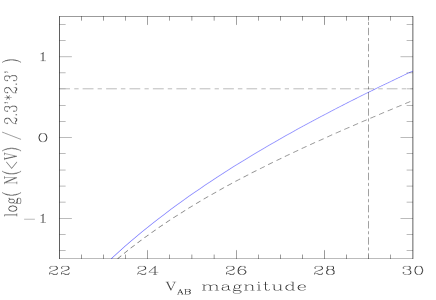
Figure 2: The quasar cumulative V-band number counts. The dashed line shows the counts of quasars with magnitude brighter than $V$ located at the redshifts $3.5<z<4.5$ while the solid line corresponds to $3.5<z<z_{ri}$.

The solid line shows the number $N(<V)$ of quasars with a magnitude lower than $V$ located at a redshift larger than $3.5$ up to the reionization redshift $z_{ri}=6.8$. The large opacity beyond this redshift prevents detection of higher $z$ objects. We also take into account the opacity due to Lyman-$\alpha$ clouds at lower $z$. We can see that our model is marginally consistent with the constraints from the HDF since it predicts $4$ detections up to $V=29$. We note that our model automatically includes photoionization feedback (threshold $T_{cool}$) and a virial temperature dependence in the relation (black hole mass) - (dark matter halo mass). However, the “cooling temperature” $T_{cool}$ is too low to have a significant effect on the number counts. Of course, we see that at bright magnitudes most of the counts come from low-redshift quasars ($z<4.5$). Thus, the QSO number counts strongly constrain our model since in order to obtain a reionization history consistent with observations (namely the HI and HeII Gunn-Peterson tests and the low-redshift amplitude of the UV background radiation field) we need a relatively large quasar multiplicity function. However, one might weaken these constraints by using an ad-hoc QSO luminosity function with many faint objects ($L_{B}<5\;10^{9}\;L_{\odot}$).

8.2 Reheating of the IGM

As we explained previously the radiation emitted by galaxies and quasars will reheat and reionize the universe, following (28) and (30). We start our calculations at $z_{i}=200$ with the initial conditions used by Abel et al.(1998), see also Peebles (1993). In particular:

$$T_{IGM}(z_{i})=\mbox{Min}\left[\;135\;\left(\frac{1+z_{i}}{100}\right)^{2}\;\mbox{K}\;,\;2.73\;(1+z_{i})\;\mbox{K}\right]$$

$$\frac{n_{HII}}{n_{H}}=2.4\;10^{-4}\;\Omega_{0}^{1/2}\;\frac{0.05}{h\Omega_{b}}$$

$$\frac{n_{H_{2}}}{n_{H}}=2\;10^{-20}\;\frac{(1-Y)\Omega_{0}^{3/2}}{h\Omega_{b}}\;(1+z_{i})^{5.1}$$

and we use a helium mass fraction $Y=0.26$. We present in Fig.3 the redshift evolution of the IGM temperature $T_{IGM}$, as well as the temperature $T_{cool}$ which defines the smallest virialized objects which can cool at redshift $z$, see (5).

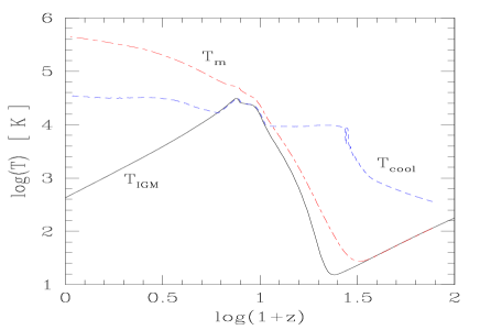
Figure 3: The redshift evolution of the IGM temperature $T_{IGM}$ (solid curve). We also show the virial temperature $T_{cool}$ of the smallest virialized halos which can cool at redshift $z$ (dashed curve) while $T_{m}$ is a mass-averaged temperature (dot-dashed curve).

At high $z$ the IGM temperature decreases with time due to the adiabatic expansion of the universe. Next, for $z<24$ ($\log(1+z)<1.4$) the medium starts being slowly reheated by the radiative output of stars and quasars until it reaches at $z\simeq 9$ a maximum temperature $T_{max}\sim 3\;10^{4}$ K where collisional excitation cooling is so efficient that the IGM temperature cannot increase significantly any more. As we shall see later, this phase occurs before the medium is reionized, as was also noticed by Gnedin & Ostriker (1997) using a numerical simulation. There is a small increase at $z\sim 7$ ($\log(1+z)\sim 0.9$) when the universe is fully reionized and the UV background radiation shows a sharp rise. However, because cooling is very efficient, the dramatic increase in $J_{\nu}$ only leads to a small change in $T_{IGM}$. Eventually at low redshifts the temperature starts decreasing again due to the expansion of the universe as the heating time-scale becomes larger than the Hubble time $t_{H}$. The temperature $T_{cool}$ which defines the smallest objects which can cool at redshift $z$ increases with time because the decline of the number density of the various species, due to the expansion of the universe, makes cooling less and less efficient. Indeed, the cooling rate (in erg cm^-3 s^-1) associated with a given process involving the species $i$ and $j$ can usually be written as $k_{ij}(T)n_{i}n_{j}$, which leads to a cooling time-scale:

$$t_{cool,ij}=\frac{3/2\;n_{b}kT}{k_{ij}(T)n_{i}n_{j}}\propto n^{-1}\sim(1+z)^{-3/2}\;t_{H}$$ (45)

where we have neglected the temperature dependence. Thus, the ratio (cooling time)/(Hubble time) increases as time goes on (at fixed $T$ and abundance fractions). Since halos with virial temperature $T_{cool}$ must satisfy $t_{cool}\sim t_{H}$, see (5), $T_{cool}$ has to get higher with time to increase the rate $k_{ij}$ (which usually contains factors of the form $\exp(-T_{ij}/T)$). The sudden increase of $T_{cool}$ at $z\sim 30$ ($\log(1+z)\sim 1.5$) is due to the decline of the fraction of molecular hydrogen which starts being destroyed by the radiation emitted by stars and quasars. As a consequence the main cooling process becomes collisional excitation cooling instead of molecular cooling. Since the former is only active at high temperatures (the coefficient rate $k(T)$ contains a term $\exp(-118348K/T)$ instead of $\exp(-512K/T)$ for molecular cooling) the cooling temperature $T_{cool}$ has to increase up to $T_{cool}\sim 10^{4}$ K. By definition $T_{cool}$ is larger than the IGM temperature and usually much higher as can be seen in Fig.3. However, at $z\sim 9$ when $T_{IGM}\sim 10^{4}$ K is quite high due to reheating by the background radiation field we have $T_{cool}=T_{IGM}$ since the IGM temperature is large enough to allow for efficient cooling. Then all virialized bound objects, with $T>T_{IGM}$, form baryonic clumps which can cool. The temperature $T_{m}$ represents a mass-averaged temperature: the matter within the IGM is associated to $T_{IGM}$ while virialized objects (hence with $T>T_{IGM}$) are characterized by a temperature defined as Min$(T,10^{6}\mbox{K})$. Since $T_{m}$ does not enter any of our calculations used to obtain the redshift evolution of the universe this crude definition is sufficient for our purpose which is merely to illustrate the difference between volume ($T_{IGM}$) and mass averages. As can be seen from Fig.3 we always have $T_{m}\geq T_{IGM}$ as it should be. At large redshifts $T_{m}\simeq T_{IGM}$ since most of the matter is within the uniform IGM component, whereas at low redshifts $z<5$ ($\log(1+z)<0.8$) the IGM temperature declines as we explained previously while $T_{m}$ remains large since most of the matter is now embedded within collapsed objects where shock heating is important (and they do not experience adiabatic cooling due to the expansion).

We show in Fig.4 the cooling and heating times associated with various processes for the IGM as well as for the smallest halos $M_{cool}$ which can cool at $z$.

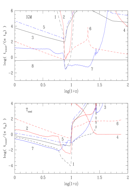
Figure 4: The cooling and heating times associated with the various relevant processes in units of $s\;t_{H}(z)$ for the IGM (upper figure) and the halos defined by $T_{cool}$ (lower figure). The labels are as follows: 1) collisional excitation, 2) collisional ionization, 3) recombination, 4) molecular hydrogen, 5) bremsstrahlung, 6) Compton, 7) photoionization heating and 8) cooling due to expansion (only for the IGM, see text).

We can see in the upper panel that for large and small redshifts, $z>24$ ($\log(1+z)>1.4$) and $z<5$ ($\log(1+z)<0.8$), all time-scales associated with the IGM are larger than the Hubble-time which means that the IGM temperature declines due to the adiabatic cooling entailed by the expansion of the universe. However, at intermediate redshifts $z\sim 18$ ($\log(1+z)\sim 1.3$) the smallest time-scale corresponds to heating by the background radiation ($t_{heat}$) which means that $T_{IGM}$ increases during this period. Next, at $z\sim 9$, the IGM temperature becomes large enough to activate collisional excitation cooling so as to reach a temporary equilibrium where $t_{cool}\simeq t_{heat}$ while $T_{IGM}$ remains constant. Then, as we shall see later the universe gets suddenly reionized at $z_{ri}=6.8$ ($\log(1+z)=0.9$). This means that $t_{heat}$ increases sharply as $n_{HI}$ declines (as well as $n_{HeI}$ and $n_{HeII}$) as can be seen from (29). The cooling time due to collisional excitation follows this rise as the medium remains in quasi-equilibrium while the temperature declines slightly (the strong temperature-dependent factors like $\exp(-118348K/T)$ in $t_{cool}$ ensure it immediately adjusts to $t_{heat}$, moreover these cooling rates are also proportional to $n_{HI}$, $n_{HeI}$ and $n_{HeII}$) until both heating and cooling time-scales become larger than the Hubble time. Then this quasi-equilibrium regime stops as the medium merely cools because of the expansion of the universe. These various phases, which appear very clearly in Fig.4, explain the behaviour of $T_{IGM}$ shown in Fig.3 which we described earlier. The peak at $z\simeq 19$ ($\log(1+z)\simeq 1.3$) of $t_{Compton}$ in the upper panel (curve 6) corresponds to the time when its sign changes (hence $t_{Compton}^{-1}=0$). At higher redshifts $T_{IGM}$ is lower than the CMB temperature (due to adiabatic cooling by the expansion of the universe), so that the gas is heated by the CMB photons while at lower $z$ the IGM temperature is larger than $T_{CMB}$ (due to reheating) so that the gas is cooled by the interaction with the CMB radiation.

The lower panel shows the cooling and heating times associated with the halos $T_{cool}$. As we have already explained we can see that at high redshifts the main cooling process is molecular hydrogen cooling. Note however that for the IGM this process is always irrelevant. This difference comes from the fact that the larger density and temperature of these virialized halos allow them to form more molecular hydrogen than is present in the IGM, so that molecular cooling becomes efficient. This was also described in detail in Tegmark et al.(1997) for instance. Of course at these redshifts we have $t_{cool,mol}=s\;t_{H}$ by definition of $T_{cool}$. Then, at $z<27$ ($\log(1+z)<1.4$) as molecular hydrogen starts being destroyed by the background radiation the main cooling process becomes collisional excitation. Note that the corresponding cooling time gets smaller than $s\;t_{H}$ because the medium is also heated by the radiation so that the actual cooling time results from a slight imbalance between cooling and heating processes. The sharp decrease of the various time-scales at $z\simeq 9$ corresponds to a sudden increase of $T_{cool}$ due to the rise of $T_{IGM}$ (which influences the cooling halos since $T_{cool}\geq T_{IGM}$) also seen in Fig.3 and in the upper panel of Fig.4. Around $z\sim 8$ ($\log(1+z)\sim 0.9$) we have $t_{cool}\ll t_{heat}$ and $t_{cool}\ll t_{H}$ so that all virialized halos above $T_{IGM}$ can cool ($T_{cool}=T_{IGM}$). The feature at $z\sim 5.3$ ($\log(1+z)\sim 0.8$) is due to reionization.

Finally, we present in Fig.5 the characteristic masses we encounter. The mass $M_{d}$ is obtained from (22):

$$M_{d}=(1+\Delta)_{IGM}\;\overline{\rho}\frac{4\pi}{3}R_{d}^{3}$$ (46)

while $M_{cool}$ corresponds to the halos which can cool at redshift $z$, as we have already explained. The mass $M_{vir}$ which follows closely the behaviour of $M_{d}$ describes the smallest virialized objects. It differs from $M_{d}$ because the density contrast is now $\Delta_{c}$ instead of $\Delta_{IGM}$. The mass $M_{NL}$ corresponds to the first non-linear scale defined by $\overline{\xi}=1$. Note that after reionization $M_{d}\sim 3\;10^{6}M_{\odot}$ while the usual Jeans mass would be $M_{J}\sim 10^{8}M_{\odot}$. This is mainly due to the low density $(1+\Delta)_{IGM}$ of the IGM, see (46) and Fig.13 below.

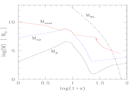
Figure 5: The redshift evolution of the characteristic masses $M_{d}$, $M_{vir}$, $M_{cool}$ and $M_{NL}$ in $M_{\odot}$.

By definition we have $M_{d}<M_{vir}\leq M_{cool}$. At $z\sim 9$ we have $M_{cool}=M_{vir}$ since $T_{cool}=T_{IGM}$ as we noticed earlier in Fig.3. We also note that at large $z$ our calculation is not entirely correct since our multiplicity functions are valid in the non-linear regime, for masses $M\ll M_{NL}$. However, at these early times the universe is nearly exactly uniform (by definition !) so that this is not a very serious problem. We can see that the first cooled objects which form in significant numbers are halos of dark-matter mass $M\sim 10^{5}M_{\odot}$ which appear at $z\sim 49$ ($\log(1+z)\sim 1.7$), when $M_{cool}$ becomes smaller than $M_{NL}$. However, they only influence the IGM after $z<24$ ($\log(1+z)<1.4$) when reheating begins.

8.3 Reionization of the IGM

After the radiation emitted by quasars and stars reheats the universe, as described in the previous section, it will eventually reionize the IGM. We present in Fig.6 the evolution with redshift of the background radiation field and of the comoving stellar formation rate. Within the framework of our model the latter is a good measure of the radiative output from galaxies, see (12), as well as from quasars, see (17), since we note that the quasar mass happens to be roughly proportional to the stellar mass.

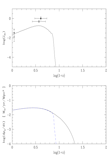
Figure 6: The redshift evolution of the UV flux $J_{21}$ (upper panel) and of the comoving star formation rate $d\rho_{s}/dt$ (lower panel). The data points are from Giallongo et al.(1996) (square), Cooke et al.(1997) (filled square), Vogel et al.(1995) (triangle, upper limit), Donahue et al.(1995) (filled triangle, upper limit) and Kulkarni & Fall(1993) (circle). The dashed line in the lower panel shows the effect of the absorption of high energy photons by the neutral hydrogen present in the IGM and in Lyman-$\alpha$ clouds.

The upper panel of Fig.6 shows the UV flux $J_{21}$ in units of $10^{-21}$ erg cm^-2 s^-1 Hz^-1 sr^-1 defined by (38). We can see that the UV flux rises very sharply at $z\simeq 6.8$ ($\log(1+z)\simeq 0.9$) which corresponds to the reionization redshift $z_{ri}$ when the universe suddenly becomes optically thin, so that the radiation emitted by stars and quasars at large frequencies is no longer absorbed and contributes directly to $J_{\nu}$. This appears clearly from the lower panel. Here the solid line shows the comoving star formation rate, obtained from (10), while the dashed line shows the same quantity multiplied by a luminosity-weighted opacity factor $\exp(-\tau_{L})$ which describes the opacity due to the IGM and Lyman-$\alpha$ clouds (see below (51), (52) and Fig.10). Thus, we can see that while the star formation rate evolves rather slowly with $z$ the absorption term varies sharply around $z_{ri}$. Hence the universe is suddenly reionized at $z_{ri}$ (when the ionized bubbles overlap: $Q_{HII}=1$) on a time-scale very short as compared to the Hubble time because of the strongly non-linear effect of the opacity. We note that for $z<1$ our star-formation model is somewhat simplified, as we explained earlier, because we defined all galaxies by a constant density contrast $\Delta_{c}$ while cooling constraints should be taken into account, as in VS II, and we also used approximations for the stellar content of galaxies which are not strictly valid for all galactic halos at these low redshifts. The reader is referred to VS II for a more precise description of the low $z$ behaviour. However, our present treatment is sufficient for our purposes and still provides a reasonable approximation at $z<1$.

We display in Fig.7 the background radiation spectrum $J_{\nu}$ at four redshifts: $z_{1}=7.3$ (before reionization), $z_{2}=6.4$ (after reionization), $z_{3}=3$ and $z_{4}=0$.

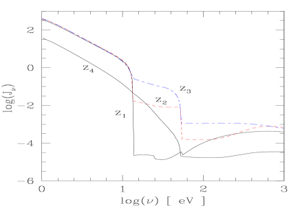
Figure 7: The background radiation spectrum $J_{\nu}$ (in units of $10^{-21}$ erg cm^-2 s^-1 Hz^-1 sr^-1) at the redshifts $z_{1}=7.3$ (solid line, prior to reionization), $z_{2}=6.4$ (lower dashed line, after reionization), $z_{3}=3$ (upper dashed line) and $z_{4}=0$ (solid line).

We see that the ionization edges corresponding to HI, HeI and HeII can be clearly seen at high $z$ before the universe is reionized. Then the background radiation is very strongly suppressed for $\nu>13.6$ eV due to HI and HeI absorption. Of course at very large frequencies $\nu\ga 1$ keV where the cross-section gets small we recover the slope $J_{\nu}\propto\nu^{-\alpha}$ of the radiation emitted by quasars. At low redshifts $z<z_{ri}$ after reionization the drop corresponding to HeI disappears as HeI is fully ionized and its number density gets extremely small, as we shall see below in Fig.9. However, even at $z\sim 3$ the ionization edges due to HI and HeII are clearly apparent and $J_{\nu}$ is still significantly different from a simple power-law. At low redshifts $z\sim 0$ the background radiation is much smoother since its main contribution comes from radiation emitted while the universe was ionized and optically thin. However, its intensity is smaller than at $z\sim 4$ because the quasar luminosity function drops at low $z$, see Fig.1, while the universe keeps expanding.

We show in Fig.8 the redshift evolution of the ionization and recombination times $t_{ion}$ and $t_{rec}$ of the IGM, divided by $t_{H}$.

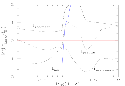
Figure 8: The redshift evolution of the ionization and recombination times $t_{ion}$ (solid line) and $t_{rec,IGM}$ (dashed line) of the IGM, divided by the Hubble time $t_{H}$. The horizontal solid line only shows $t_{H}$ for reference. The recombination times $t_{rec,mean}$ (uniform medium) and $t_{rec,bubble}$ (ionized bubbles) are defined in the main text.

More precisely, the ionization time $t_{ion}$ is defined by:

$$t_{ion}^{-1}=\int 4\pi\;\frac{J_{\nu}}{h\nu}\;\sigma_{HI}(\nu)\;d\nu$$ (47)

while the recombination time within the IGM is:

$$t_{rec,IGM}^{-1}=\alpha(T_{IGM})\;C_{n}\;\overline{n}_{e-}$$ (48)

where $\alpha$ is the recombination rate, $C_{n}$ the clumping factor and $\overline{n}_{e-}$ the mean electron number density, from (27) and (26). We also display for reference the recombination time which would correspond to a uniform medium with the mean density of the universe:

$$t_{rec,mean}=(1+\Delta)_{n}\;C_{n}\;t_{rec,IGM}$$ (49)

Finally, we show the recombination time within ionized bubbles (where all hydrogen atoms are ionized):

$$t_{rec,bubble}^{-1}=\alpha\left(3\;10^{4}\mbox{K}\right)\;C_{n}\;\overline{n}_{H}$$ (50)

The recombination time grows with time at high $z$ as the mean density decreases with the expansion, although this is somewhat balanced by the increase of the clumping factor $C_{n}$ (see below Fig.13). In particular, the decrease of $t_{rec,IGM}$ around $z\sim 30$ ($\log(1+z)\sim 1.5$) is due to the growth of $C_{n}$. The sharp drop at $z\sim 7$ ($\log(1+z)\sim 0.9$) is due to reionization which suddenly increases the number density of free electrons. After reionization the recombination time characteristic of the IGM keeps decreasing (while $t_{rec,mean}$ increases slightly since the density declines) because of the growth of the clumping factor $C_{n}$, see Fig.13, which overides the decline of the mean universe density. The recombination time within ionized bubbles $t_{rec,bubble}$ follows the change of the mean universe density and of the clumping factor $C_{n}$. At large $z$ it is much smaller than the mean IGM recombination time since the IGM is close to neutral. At low $z$ it becomes larger than $t_{rec,IGM}$ since the IGM is suddenly reionized with a temperature $T_{IGM}$ which declines after reheating and gets lower than $3\;10^{4}$ K, see Fig.3. The ionization time is very large at high $z$ since the UV background radiation is small. Then it decreases very sharply at $z_{ri}$ when the universe is reionized and the background radiation suddenly grows as the medium becomes optically thin, as seen in Fig.6. The reionization redshift corresponds to the time when $t_{ion}$ becomes smaller than $t_{H}$, somewhat after it gets smaller than $t_{rec,IGM}$. Thus $t_{rec,IGM}$ does not play a decisive role since it is never the smallest time-scale around reionization.

Finally, we show in Fig.9 how the chemistry of the IGM evolves with time as the temperature $T_{IGM}$ and the UV flux $J_{21}$ vary with $z$.

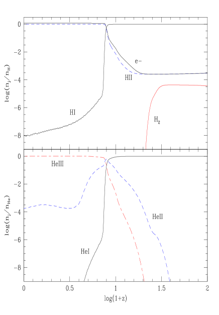
Figure 9: The redshift evolution of the chemistry of the IGM. The upper panel shows the ionization state of hydrogen, as well as the fraction of molecular hydrogen and electrons. The lower panel presents the ionization of helium.

We see very clearly in the upper panel the redshift of reionization $z_{ri}=6.8$ ($\log(1+z)=0.9$) when the fraction of neutral hydrogen $n_{HI}/n_{H}$ declines very sharply while the UV flux $J_{21}$ suddenly rises, as was shown in Fig.6. We note that at low redshifts $z<z_{ri}$ the neutral hydrogen fraction decreases more slowly down to $n_{HI}/n_{H}\sim 10^{-8}$. The fractions of electrons and ionized hydrogen start increasing earlier at $z\sim 19$ ($\log(1+z)\sim 1.3$) but of course they remain small until $z_{ri}$. The abundance of molecular hydrogen decreases sharply at a rather high redshift $z\sim 27$ ($\log(1+z)\sim 1.4$) due to the background radiation, as we noticed on Fig.4. The lower panel shows that helium gets fully ionized simultaneously with hydrogen. In particular, although there remains a small fraction of HeII ($\sim 10^{-4}$) the abundance of HeI gets extremely small. We note that at low redshifts $z<2$ the fraction of HeII does not evolve much (and even slightly increases) while the HI abundance keeps declining. This is due to the fact that the radiation relevant for helium ionization comes from quasars whose luminosity function drops at low $z$ as shown in Fig.1 while an important contribution to the hydrogen ionizing radiation is provided by stars and the galaxy luminosity function declines more slowly with time at low $z$, as seen in Fig.6 or in VS II. We shall come back to this point in Sect.8.7.

8.4 Opacities

As we explained previously the radiation emitted by stars and quasars at high frequencies ($\nu>13.6$ eV) is absorbed by the IGM and discrete clouds as it propagates into the IGM. This leads to the extinction factors $\exp(-\tau_{s}(x))$ and $\exp(-\tau_{Q}(x))$ in the evaluation of the source terms (13) and (21) for the background radiation. We define here the “luminosity averages” $\tau^{L}_{IGM,NHI}$ for both continuous and discrete components by:

$$e^{-\tau^{L}}=\left(\frac{d\rho_{s}}{dt}\right)^{-1}\;\int\eta_{g}(x)\;\frac{dx}{x}\;\left(\frac{dM_{s}}{dt}\right)(x)\;e^{-\tau_{s}(x)}$$ (51)

where $\tau_{s}(x)$ is the relevant opacity (from the IGM or clouds for sources $x$, see (44) ) at the frequency 20 eV below the HeI ionization threshold without taking into account the factors $Q_{HI}$ which describe ionized bubbles. The subscript $s$ refers to the fact that we consider here the opacity which enters into the calculation of the stellar radiative output. The quasar-related opacity mainly differs through the factor $\lambda_{Q}$, see (42). The weight $dM_{s}/dt$ corresponds to a luminosity weight as we noticed earlier, see (12), (17) and (6).

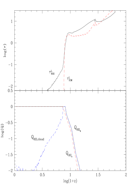
Figure 10: Upper panel: the redshift evolution of the opacity from the IGM (dashed line) and “Lyman-$\alpha$ clouds” (solid line) which enters the absorption factors in the calculation of the radiative output from stars and quasars. Lower panel: evolution of the filling factors $Q_{HII_{Q}}$ (ionized bubbles around quasars, solid line), $Q_{HII_{s}}$ (around galaxies, upper dashed line) and $Q_{HII,cloud}$ (lower dashed line).

We show in the upper panel of Fig.10 the redshift evolution of the opacity from the IGM ($\tau^{L}_{IGM}$, dashed line) and from “Lyman-$\alpha$ clouds” ($\tau^{L}_{NHI}$, solid line). We can see that both contributions have roughly the same magnitude before reionization, except at very high redshifts $z>50$ ($\log(1+z)>1.7$) when very few structures exist as shown in Fig.12. Prior to reionization the opacity is large and the background radiation quite small, as seen in Fig.6. At $z_{ri}$ the opacity suddenly declines while $J_{21}$ rises sharply, due to the strong non-linear coupling between $\tau$ and $J_{\nu}$, as we explained in the lower panel of Fig.6 where we presented the influence of the total opacity $\tau_{L}$:

$$\tau_{L}=\tau^{L}_{IGM}+\tau^{L}_{NHI}$$ (52)

At low redshifts $z<z_{ri}$ when the universe is reionized the opacity due to discrete clouds becomes much larger than the IGM contribution (although it is very small) because the density of neutral hydrogen is now proportional to the square of the baryonic density (in photoionized regions) and most of the matter is embedded within collapsed objects.

The opacities $\tau^{L}$ were shown in the upper panel of Fig.10 without the filling factors $Q_{HI}$ which enter the actual evaluation of the source terms (13) and (21), see (40). The filling factors $Q_{HII}$, describing the volume fraction occupied by ionized bubbles, are shown in the lower panel of Fig.10. We can see that $Q_{HII_{s}}$ and $Q_{HII_{Q}}$ increase with time as structures form and emit radiation while the IGM density declines. When these ionized bubbles overlap ($Q_{HII}=1$) the universe is reionized. At low redshifts the coefficient $Q_{HII,cloud}$ declines because the background radiation is large while the quasar number density drops (indeed $Q_{HII,cloud}$ measures the volume occupied by the “spheres of influence” of quasars).

Next, we can evaluate the mean opacities $\tau_{HI}(z)$ and $\tau_{HeII}(z)$ seen on a random line of sight from $z=0$ to a quasar located at redshift $z$. We present in Fig.11 the contributions from both the uniform IGM component and the discrete Lyman-$\alpha$ clouds.

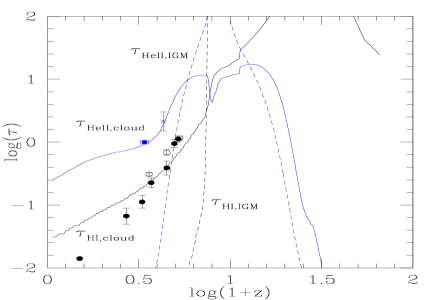
Figure 11: The redshift evolution of the average opacities $\tau_{HI}$ and $\tau_{HeII}$ along a random line of sight produced by “Lyman-$\alpha$ clouds”. The dashed lines show the opacities from the uniform IGM. The data points are from Press et al.(1993) (circles), Zuo & Lu (1993) (filled circles) for hydrogen, and from Davidsen et al.(1996) (filled rectangle) and Hogan et al.(1997) (cross) for helium.

At high redshifts prior to reionization the main contribution to the opacity is provided by the IGM which contains most of the matter. However, at low $z$ when the IGM is ionized most of the absorption comes from the Lyman-$\alpha$ clouds. At large $z$ the HeII opacity is very small because most of the helium is in its neutral form HeI. We refer the reader to Valageas et al.(1999a) for a much more detailed description of the properties of the Lyman-$\alpha$ clouds at low $z$. We can see that our predictions show a reasonable agreement with observations for the hydrogen opacity. At low redshifts $z<1$ the influence of star-formation which consumes and may eject some of the gas (which we did not take into account here) could explain the relatively high opacity we obtain. The helium opacity we find is also close to observations. This is due to the fact that the UV radiation spectrum shows strong ionization edges, even at relatively low redshifts $z\sim 3$ ($\log(1+z)\sim 0.6$), see Fig.7. Hence the ratio $N_{HeII}/N_{HI}$ is rather large, see Fig.9, which explains why we get a better agreement than Zheng et al.(1998) for instance (see also Valageas et al.1999a). In particular, we have $n_{HeII}/n_{HeIII}\gg n_{HI}/n_{HII}$ since $n_{HeII}/n_{HeIII}\sim 10^{-4}$ while $n_{HI}/n_{HII}\sim 10^{-8}$ at low redshift. We note that the observed HeII opacity strongly constrains the quasar contribution to the reionization process since stellar radiation is small at high frequencies (due to the near blackbody behaviour of stellar spectra). In particular, it implies that one needs a population of faint QSOs ($M_{B}>-26.7$) in order to reionize helium but $z_{ri}$ should not be too large so that there is still an appreciable density of HeII. In other words, as we noticed above, the UV radiation field must still display strong ionization edges, which means that it has not had enough time to be smoothed out by the radiation emitted since $z_{ri}$ when the medium is optically thin.

8.5 Stellar properties

Our model also allows us to obtain the fraction of matter within virialized or cooled halos, as well as in stars.

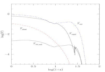
Figure 12: The redshift evolution of the fraction of matter enclosed within virialized halos ($F_{vir}$), cooled objects ($F_{cool}$) and stars ($F_{star}$). The lower solid line is the volume fraction $F_{vir,vol}$ occupied by virialized objects.

We show in Fig.12 the fraction of matter within virialized halos ($F_{vir}$, upper dashed line), cooled objects ($F_{cool}$, upper solid line) and stars ($F_{star}$, lower dashed line). The first two quantities are simply obtained from (3). Of course we have: $F_{star}\leq F_{cool}\leq F_{vir}$. Around $z\sim 9$ we note that $F_{cool}=F_{vir}$ because as we explained previously at this time all virialized objects (with $T\geq T_{IGM}$) can cool efficiently ($T_{cool}=T_{IGM}$). The fraction of matter within virialized halos increases very fast at high redshifts $z\sim 49$ ($\log(1+z)\sim 1.6$) as $M_{vir}$ becomes smaller than $M_{NL}$, see Fig.5, when dark matter structures form on scale $R_{d}$. However, until $z\sim 15$ ($\log(1+z)\sim 1.2$) the mass within cooled halos remains much smaller because cooling is not very efficient so that $T_{cool}\gg T_{IGM}$, see Fig.3. At low redshifts $z<5$ ($\log(1+z)<0.8$) both $F_{vir}$ and $F_{cool}$ get close to unity since most of the matter is now embedded within collapsed and cooled halos (even though $T_{cool}$ becomes again much larger than $T_{IGM}$: we are so far within the non-linear regime that even $T_{cool}$ is small compared to the characteristic virial temperature of the structures built on scale $R_{d}$). Of course the mass within stars grows with time, closely following $F_{cool}$. Note however that it is not strictly proportional to $F_{cool}$ since an increasingly large fraction of the gas within galaxies is consumed into stars. The fraction of volume $F_{vir,vol}$ occupied by virialized objects always remains small as it satisfies:

$$F_{vir,vol}=\frac{1}{1+\Delta_{c}}\;F_{vir}\leq\frac{1}{1+\Delta_{c}}$$ (53)

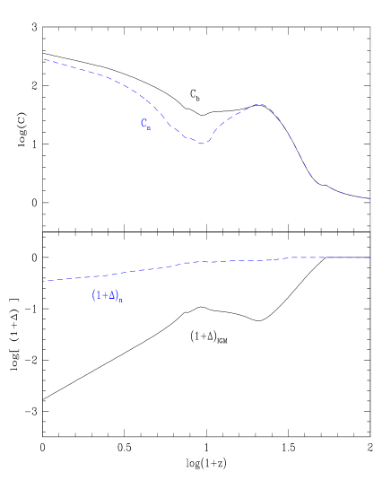
Figure 13: Upper panel: the redshift evolution of the clumping factors $C_{b}$ and $C_{n}$. Lower panel: the overdensities $(1+\Delta)_{IGM}(z)$ characteristic of most of the volume of the universe at redshift $z$ at scale $R_{d}$ and $(1+\Delta)_{n}$.

We show in the upper panel of Fig.13 the clumping factor $C_{b}$ defined by (25). The expression (25) shows clearly that at large redshifts where there are very few collapsed baryonic structures $C_{b}\simeq 1$ while at low $z$ when most of the baryonic matter is within virialized halos (note this is always true for dark matter on sufficiently small scales) we have $C_{b}\simeq\Delta_{c}$. We can see in the figure that $C_{b}$ usually increases with time as the hierarchical clustering process goes on. The temporary decrease at $z\sim 15$ ($\log(1+z)\sim 1.2$), which also appears in the lower panel and in Fig.12, is due to the reheating of the universe, shown in Fig.3, which increases the “damping” length $R_{d}$ and mass scale $M_{d}$, as seen in Fig.5. As a consequence, small objects which were previously well-defined entities suddenly see the IGM temperature become larger than their virial temperature. Hence they cannot retain efficiently their gas content and they lose their identity. We note that neglecting the clumping of the gas would lead to a higher reionization redshift $z_{ri}=7.3$ since it would underestimate the efficiency of recombination. The clumping factor $C_{n}$ displays a behaviour similar to $C_{b}$ but it is usually smaller since it does not include the deep halos which can cool. We display in the lower panel of Fig.13 the overdensity $(1+\Delta)_{IGM}(z)$ characteristic of most of the volume of the universe at redshift $z$ when seen on scale $R_{d}$. While structures form and the matter gets embedded within overdensities which occupy a decreasing fraction of the volume (when seen at this scale $R_{d}$) the “overdensity” $(1+\Delta)_{IGM}$ which characterises the medium in-between these objects (halos or filaments) declines. The density contrast $(1+\Delta)_{n}$ which corresponds to the IGM and shallow potential wells which do not form stars (but constitute Lyman-$\alpha$ clouds) decreases more slowly since it only excludes the high virial temperature halos with $T>T_{cool}$.

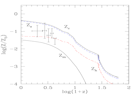
Figure 14: The redshift evolution of the metallicities $Z_{c}$ (star-forming gas), $Z_{s}$ (stars), $Z_{h}$ (galactic halos) and $Z_{m}$ (matter average). The data points are from Pettini et al.(1997) for the zinc metallicity of damped Lyman-$\alpha$ systems.

We present in Fig.14 the redshift evolution of the mean metallicities (in units of solar metallicity) $Z_{c}$ (within the star-forming gas located in the inner parts of galaxies, upper solid line), $Z_{s}$ (within stars, upper dashed line) and $Z_{h}$ (within galactic halos, lower dashed line). We use the mass average over the various galactic halos:

$$Z=\frac{\int Z(M)\;\mu_{g}(M)\;\frac{dM}{M}}{\int\mu_{g}(M)\;\frac{dM}{M}}$$ (54)

where $\mu_{g}(M)dM/M$ is the galaxy mass function defined as in (3). The reader is referred to VS II for a detailed description of these metallicities (note that we only consider here the abundance of Oxygen or any other element that is mainly produced by SN II since we did not include SN I in our model). The lower solid line corresponds to a “matter averaged” metallicity $Z_{m}$ defined by $Z_{m}=F_{cool}Z_{h}$. Thus, although we do not include explicitly in our model any contamination of the IGM by heavy elements produced within galaxies, $Z_{m}$ defined in this way provides an upper bound for the mean IGM metallicity (corresponding to very efficient mixing). If galaxies do not eject metals very deeply within the IGM its metallicity could be much smaller. The mean metallicity of Lyman-$\alpha$ clouds associated to galactic halos (limit or damped systems) is $Z_{h}$. Our results agree well with observations by Pettini et al.(1997) for damped Lyman-$\alpha$ systems. Note that there is in fact a non-negligible spread in metallicity over the various halos.

8.6 Consequence for the CMB radiation

After reionization, CMB photons may be scattered by electrons present in the gas. We write the corresponding Thomson opacity up to a redshift $z$ as:

$$\tau_{es}(z)=\int_{0}^{z}c\frac{dt}{dz}\;\sigma_{T}\;\overline{n}_{e}(z)$$ (55)

where $\overline{n}_{e}(z)$ is the mean electron number density at redshift $z$. We take:

$$\overline{n}_{e}(z)=(1-Y)\;\frac{\Omega_{b}}{\Omega_{0}}\;\frac{\overline{\rho}(z)}{m_{p}}\;\left(\frac{n_{e}}{n_{H}}\right)_{IGM}$$ (56)

which means that we use the same electron fraction in clouds as for the IGM (note that we calculate the IGM electron number density together with the ionization state of hydrogen and helium). Then, CMB anisotropies are damped on angular scales smaller than the angle subtended by the horizon at reionization. We use the analytic fit given by Hu & White (1997) to obtain the damping factor $R_{l}^{2}$ of the CMB power-spectrum $C_{l}$ from the optical depth $\tau_{es}$. The results are shown in Fig.15.

Figure 15: Upper panel: the optical depth $\tau_{es}$ for electron scattering. Lower panel: damping factor $R_{l}^{2}$ for the CMB power-spectrum.

We can check that the total opacity $\tau_{es}\simeq 0.023$ is quite small because reionization occurs rather late at $z_{ri}\simeq 6.8$. This also implies that the damping factor $R_{l}^{2}$ remains close to unity: $R_{l}^{2}\simeq 0.95$ for large $l$. Another distortion of the CMB radiation is the Sunyaev-Zeldovich effect which transfers photons from the Rayleigh-Jeans part of the spectrum to the Wien tail when they are scattered by hot electrons. The magnitude of this perturbation is conveniently described by the Compton parameter $y$:

$$y(z)=\int_{0}^{z}c\frac{dt}{dz}dz\;\sigma_{T}\;n_{e}\;\frac{kT}{m_{e}c^{2}}$$ (57)

We can first consider the contribution of the IGM gas, using in (57) the temperature and the electronic density of this uniform component. Then, we estimate the distortion due to the hot gas embedded within virialized objects. We can write this latter contribution as:

$$y_{halos}=\int dy_{IGM}\;\frac{1}{(1+\Delta)_{IGM}}\;F_{vir}\;\frac{T_{mvir}}{T_{IGM}}$$ (58)

where we used the same electronic fraction for halos and the IGM. The temperature $T_{mvir}$ is the “mass averaged” temperature of virialized objects while $F_{vir}$ is the mass fraction within collapsed objects displayed in Fig.12. The results are presented in Fig.16.

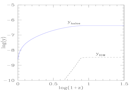
Figure 16: The Compton parameter $y$ up to redshift $z$ describing the Sunyaev-Zeldovich effect from the IGM (dashed line) and virialized halos (solid line).

The Compton parameter $y_{IGM}$ due to the IGM first increases rather fast with $z$ until reionization, together with $n_{e}$ and $T_{IGM}$. After $z_{ri}$ it reaches a plateau and does not grow any more since at these large redshifts the universe is almost exactly neutral. The contribution $y_{halos}$ of virialized objects is much larger at low $z$ than $y_{IGM}$ since the temperature of these collapsed halos is much higher than $T_{IGM}$, as shown in Fig.3. We can note however that $y_{halos}$ grows much slower and becomes close to its asymptotic value earlier than $y_{IGM}$. This is due to the fact that the characteristic temperature of virialized halos declines at larger $z$, see Fig.3, and the mass fraction they contain also decreases (while the IGM undergoes the opposite trends). A more detailed description of the Sunyaev-Zeldovich effect due to clusters, and its fluctuations (which in fact have the same magnitude as the mean), will be presented in a future article.

8.7 Contributions of quasars and stars

In our model the radiation which reheats and reionizes the universe comes from both quasars and stars. At large frequencies $\nu>24.6$ eV most of the UV flux is emitted by quasars so that stars play no role in the helium ionization. However, at lower frequencies both contributions have roughly the same magnitude. We present in Fig.17 the redshift evolution of the radiative output due to stars and quasars.

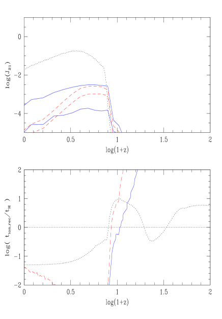
Figure 17: Upper panel: the redshift evolution of the “instantaneous” UV fluxes $J_{HI}^{i}$ and $J_{HeI}^{i}$ due to stars (solid lines) and quasars (dashed lines). The dotted line is the UV flux $J_{21}$ shown in Fig.6. Lower panel: the “instantaneous” ionization times $t_{ion;s,Q}^{i}$ due to stars (solid line) and quasars (dashed line). The dotted curve is the recombination time as in Fig.8 while the horizontal solid line is the Hubble time $t_{H}$.

Thus, we define the “instantaneous” radiation fields:

$$J_{\nu;s,Q}^{i}=\frac{1}{10}\;t_{H}\;S_{\nu;s,Q}$$ (59)

where $t_{H}(z)$ is the Hubble time, see (30). From these quantities we define the averages $J_{HI;s,Q}^{i}(z)$ and $J_{HeI;s,Q}^{i}(z)$ as in (38). This provides a measure of the radiative output above the ionization thresholds $\nu_{HI}$ and $\nu_{HeI}$ due to stars and quasars. We can also derive the ionization times $t_{ion;s,Q}^{i}$ as in (47). We can see in the upper panel that at reionization $z\sim z_{ri}$ the contributions to HI ionizing radiation from stars and quasars are of the same order. However, since the quasar spectrum is much harder than stellar radiation we have $J_{HeI;Q}^{i}\gg J_{HeI;s}^{i}$ so that quasars are slightly more efficient at reheating and reionizing the universe (the additional factor $(\nu-\nu_{j})$ in (29) increases the weight of high energy photons which also remain longer above the threshold $\nu_{HI}$ while being redshifted). At low $z$ we can see that the quasar radiative output declines much faster than the stellar source term. Of course, this is due to the sharp drop at low redshifts of the quasar luminosity function. This decrease of $S_{\nu Q}$ as compared to $S_{\nu s}$ comes from two effects: i) as time increases the “creation time-scale” of halos of the relevant masses $M\sim 10^{12}M_{\odot}$ (through merging of smaller sub-units, measured by $t_{Q}/t_{M}$) grows and ii) there is less gas available to fuel the quasars (which even disappear) while old stars can still provide a non-negligible luminosity source for galaxies. We can note in the upper panel that the redshift evolution of the background radiation field $J_{21}(z)$ actually produced by stars and quasars does not exactly follow the “instantaneous” quantities $J_{HI;s,Q}^{i}(z)$ since one must take into account the expansion of the universe and deviations from equilibrium. This explains the slower increase of $J_{21}$ at $z\sim z_{ri}$ as well as the relatively low approximate ionization times $t_{ion;s,Q}^{i}$ at this epoch.

9 Critical universe

We now consider the case of a critical universe $\Omega=1$ with a CDM power-spectrum (Davis et al.1985) normalized to $\sigma_{8}=0.5$. We also choose $\Omega_{b}=0.04$ and $H_{0}=60$ km/s/Mpc. Thus, as in the previous case of an open universe our model is consistent with the studies described in VS II and Valageas et al.(1999a).

9.1 Quasar luminosity function

We first present our results for the redshift evolution of the quasar luminosity function in Fig.18.

Figure 18: The evolution with redshift of the B-band quasar luminosity function in comoving Mpc^-3, as in Fig.1. The data points are from Pei (1995).

We can check that our results are similar to those obtained previously for an open universe and they again agree reasonably with observations. This is not very surprising since we use the same physical model so that we recover a similar behaviour. We present in Fig.19 the quasar number counts we obtain from our model.

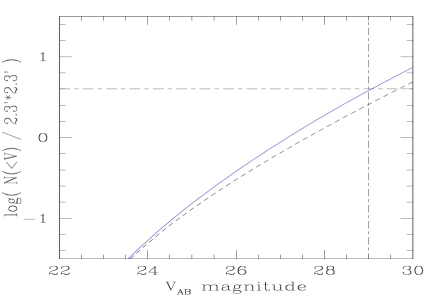
Figure 19: The quasar cumulative V-band number counts. The dashed line shows the counts of quasars with a magnitude brighter than $V$ located at redshifts $3.5<z<4.5$ while the solid line corresponds to $3.5<z<z_{ri}$.

We can see that our results are similar to those displayed previously in Fig.2 and that our predictions are still marginally consistent with the lack of observation in the HDF.

9.2 Reheating

We present in Fig.20 the redshift evolution of the IGM temperature $T_{IGM}$, the virial temperature $T_{cool}$ of the smallest objects which can cool at a given time, and the mass averaged temperature $T_{m}$.

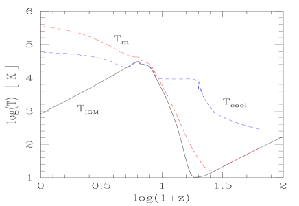
Figure 20: The redshift evolution of the IGM temperature $T_{IGM}$ (solid curve), the virial temperature $T_{cool}$ (upper dashed curve) and the mass averaged temperature $T_{m}$ (lower dashed curve), as in Fig.3.

We can see that our results are again very close to those obtained for an open universe. Indeed, the structure formation process is quite similar and it must agree with the same observations (quasar and galaxy luminosity functions, Lyman-$\alpha$ column density distribution) at low $z$.

9.3 Reionization

We display in Fig.21 the redshift evolution of the background radiation and the comoving star formation rate.

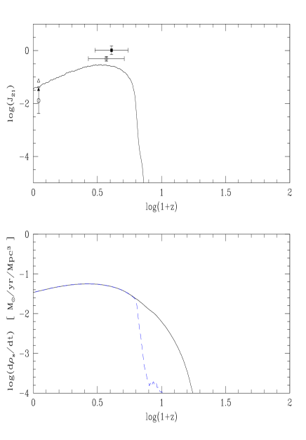
Figure 21: The redshift evolution of the UV flux $J_{21}$ (upper panel) and of the comoving star formation rate $d\rho_{s}/dt$ (lower panel) for the case of an open universe. The dashed line in the lower panel shows the effect of the absorption of high energy photons by the neutral hydrogen present in the IGM and in Lyamn-$\alpha$ clouds.

We can check that we recover the behaviour obtained previously for an open universe. However, the reionization redshift $z_{ri}=5.6$ is smaller than previously. This is related to the lower normalization $\sigma_{8}$ of the power-spectrum as compared to the previous case. This leads to fewer bright quasars at high $z$ (compare Fig.18 and Fig.1) and to a smaller radiative output.

We can also check that the hydrogen and helium reionization process is close to our previous results (as for the reheating). Thus, for most practical purposes both critical and open cosmologies allow reasonable reheating and reionization histories which are very similar. In fact, the uncertainties involved in the galaxy and quasar formation processes are probably too large to favour significantly one of these two possible scenarios (as compared to the other). However, both models are consistent with present observations.

10 Conclusion

In this article we have described an analytic model for structure formation in the universe which deals simultaneously with quasars, galaxies and Lyman-$\alpha$ clouds, within the framework of a hierarchical scenario. This allows us to study the reheating and reionization history of the universe consistently with the properties of these various classes of objects. We have shown that for both a critical and an open universe our predictions agree reasonably well with observations. However, as was noticed by Haiman et al.(1998) it appears that the observational constraints on the quasar luminosity function are already strong. Moreover, the Gunn-Peterson test for HeII provides stringent additional constraints on the quasar contribution to the UV radiation field and on the reionization redshift. Thus, although our model in its simplest version (i.e. as described here, with no additional cutoffs for the quasar multiplicity function) is marginally consistent with the data, further observations of the helium opacity and of the quasar number counts (e.g. with the NGST) could provide tight constraints on such models where reionization is produced by QSOs. On the other hand, since reionization occurs rather late $z_{ri}\leq 7$ the damping of CMB anisotropies is quite small.

We can note that our predictions are similar to some results obtained by Gnedin & Ostriker (1997) with a numerical simulation (but for a different cosmology). Moreover, the fact that our model agrees reasonably with observations for Lyman-$\alpha$ clouds, galaxies, quasars and constraints on the reionization process, strongly suggests that its main characteristics are fairly realistic. Thus, it provides a simple description of structure formation in the universe, from high redshifts after recombination down to the present epoch.

- [1]
- [2] Abel T., Anninos P., Zhang Y., Norman M.L., 1997, NewA 2, 181
- [3] Abel T., Anninos P., Norman M.L., Zhang Y., 1998, ApJ 508, 518
- [4] Anninos P., Zhang Yu, Abel T., Norman M.L., 1997, NewA 2, 209
- [5] Balian R., Schaeffer R., 1989, A&A 220, 1
- [6] Bouchet F.R., Schaeffer R., Davis M., 1991, ApJ 383, 19
- [7] Colombi S., Bernardeau F., Bouchet F.R., Hernquist L., 1997, MNRAS 287, 241
- [8] Cooke A.J., Espey B., Carswell R.F., 1997, MNRAS 284, 552
- [9] Davidsen A.F., Kriss G.A., Weizheng, 1996, Nature 380, 47
- [10] Davis M., Efstathiou G.P., Frenk C.S., White S.D.M., 1985, ApJ 292, 371
- [11] Donahue M., Aldering G., Stocke J.T., 1995, ApJL 450, L45
- [12] Efstathiou G., Rees M.J., 1988, MNRAS 230, 5p
- [13] Elvis M., Wilkes B.J., McDowell J.C., Green R.F., Bechtold J., Willner S.P., Oey M.S., Polomski E., Cutri R., 1994, ApJS 95, 1
- [14] Giallongo E., Cristiani S., D’Odorico S., Fontana A., Savaglio S., 1996, ApJ 466, 46
- [15] Gnedin N.Y., Ostriker J.P., 1997, ApJ 486, 581
- [16] Haiman Z., Loeb A., 1997, ApJ 483, 21
- [17] Haiman Z., Loeb A., 1998, ApJ 503, 505
- [18] Haiman Z., Madau P., Loeb A., 1998, submitted to ApJ, astro-ph 9805258
- [19] Hogan C.J., Anderson S.F., Rugers M.H., 1997, AJ 113, 1495
- [20] Kauffmann G., White S.D.M., Guiderdoni B., 1993, MNRAS 264, 201
- [21] Kulkarni V.P., Fall S.M., 1993, ApJL 413, L63
- [22] McKee C.F., 1989, ApJ 345, 782
- [23] McLow M-M, Ferrara A., 1998, astro-ph 9801237
- [24] Magorrian J., Tremaine S., Richstone D., Bender R., Bower G., Dressler A., Faber S.M., Gebhardt K., Green R., Grillmair C., Kormendy J., Lauer T., 1998, AJ 115, 2285
- [25] Nusser A., Silk J., 1993, ApJ 411, L1
- [26] Peebles P.J.E., 1993, Principles of Physical Cosmology, Princeton University Press, NJ
- [27] Pei Y.C., 1995, ApJ 438, 623
- [28] Pettini M., Smith L.J., King D.L., Hunstead R.W., 1997, ApJ 486, 665
- [29] Press W., Schechter P., 1974, ApJ 187, 425
- [30] Press W.H., Rybicki G.B., Schneider D.P., 1993, ApJ 414, 64
- [31] Shapiro P.R., Giroux M.L., 1987, ApJ 321, L107
- [32] Tegmark M., Silk J., Rees M.J., Blanchard A., Abel T., Palla F., 1997, ApJ 474, 1
- [33] Valageas P., Schaeffer R., 1997, A&A 328, 435 (VS I)
- [34] Valageas P., Schaeffer R., 1998, accepted by A&A, astro-ph 9812213 (VS II)
- [35] Valageas P., Schaeffer R., Silk J., 1999a, accepted by A&A, astro-ph 9903388
- [36] Valageas P., Lacey C., Schaeffer R., 1999b, submitted to MNRAS, astro-ph 9902320
- [37] Vogel S.N., Weymann R., Rauch M., Hamilton T., 1995, ApJ 441, 162
- [38] Zheng W., Davidsen A.F., Kriss G.A., 1998, AJ 115, 319
- [39] Zuo L., Lu L., 1993, ApJ 418, 601