THE REFLEX CLUSTER SURVEY: OBSERVING STRATEGY AND FIRST RESULTS ON LARGE–SCALE STRUCTURE

1 Introduction

As a modern version of ancient cartographers, during the last 20 years cosmologists have been able to construct more and more detailed maps of the large–scale structure of the Universe, as delineated by the distribution of galaxies in space. This has been possible through the development of redshift surveys, whose efficiency in covering ever larger volumes has increased exponentially thanks to the parallel evolution in the performances of spectrographs and detectors (see e.g. Da Costa 1998 and Chincarini & Guzzo 1998, for recent reviews of the historical development of this field).

While the most recent projects, as the Las Campanas Redshift Survey (LCRS, Shectman et al. 1996) and the ESO Slice Project (ESP, Vettolani et al. 1997) have considerably enlarged our view by collecting several thousands of redshifts out to a depth of $\sim 500\rm\,h^{-1}\,Mpc$ , the quest for mapping a “fair sample” of the Universe is not yet fully over. These modern galaxy redshift surveys have indeed been able to show for the first time that large–scale structures such as surperclusters and voids keep sizes which are smaller than those of the surveys themselves (i.e. $\sim 100-200\rm\,h^{-1}\,Mpc$). This is in contrast to the situation only a few years ago, when every new redshift survey used to discover newer and larger structures (a famous case was the “Great Wall”, spanning the whole angular extension of the CfA2 survey, see Geller & Huchra 1989). On the other hand, it has also been realised from the ESP and LCRS results, among others, that to characterise statistically the scales where the Universe is still showing some level of inhomogeneity, surveys covering much larger areas to a similar depth ($z\sim 0.2$), are necessary.

To fulfill this need on one side two very ambitious galaxy survey projects have started, the Sloan Digital Sky Survey (SDSS, Margon 1998) and the 2dF Redshift Survey (Colless 1999). The SDSS in particular, including both a photometric survey in five filters and a redshift survey of a million galaxies over the whole North Galactic cap, represents a massive effort involving the construction of a dedicated telescope with specialised camera and spectrograph.

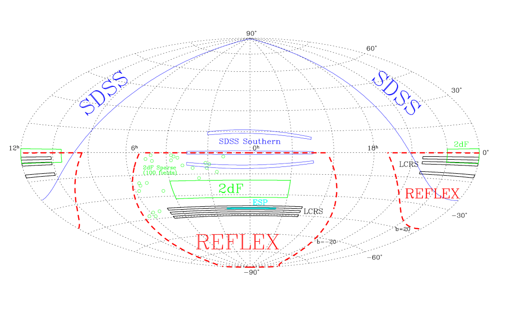
Figure 1: Aitoff view of how wide–angle redshift surveys with typical depth of $z\sim 0.2$ are covering the available sky (see Guzzo 1999 for details).

Alternatively, one could try to cover similar volumes using a different tracer of large–scale structure, one requiring a more modest investment in telescope time, so that a survey can be performed using standard instrumentation and within the restrictions of public telescopes as those of ESO. This has been the strategy of the REFLEX Key Programme, that uses clusters of galaxies to cover, in the Southern hemisphere, a volume of the Universe comparable to that of the SDSS in the North. Clusters, being rarer than galaxies, are evidently more efficient tracers for mapping very large volumes. The price to pay is obviously that of loosing resolution in the description of the small–scale details of large–scale structure. However such information is already provided by the present generation of galaxy surveys.

The REFLEX cluster survey, in particular, is based on clusters selected through their X–ray emission, which is a more direct probe of their mass content than simple counts of galaxies, i.e. richness. Therefore, using clusters as tracers of large–scale structure, not only do we sample very large scales in an observationally efficient way, but if we select them through their X–ray emission we also have a more direct relation between luminosity and mass. Further benefits of the extra information provided by the X-ray emission have been discussed in our previous Messenger article (Böhringer et al. 1998). In the same paper, we also presented details on the cluster selection, the procedure for measuring of X-ray fluxes, and some properties of the objects in the catalogue, as the X-ray luminosity function, together with a first determination of the power spectrum. Results on the cluster X-ray luminosity function have also been obtained during the development of the project from an early pilot subsample at bright fluxes (see De Grandi et al. 1999). Here we would like to concentrate on the key features of the optical follow-up observations at ESO, and then present more results on the large-scale distribution of REFLEX clusters and their clustering properties. Nevertheless, for the sake of clarity we shall first briefly summarise the general features of the survey.

2 The REFLEX Cluster Survey

The REFLEX (ROSAT-ESO Flux Limited X-ray) cluster survey combines the X–ray data from the ROSAT All Sky Survey (RASS), and ESO optical observations to construct a complete flux–limited sample of about 700 clusters with measured redshifts and X-ray luminosities. The survey covers almost the southern celestial hemisphere (precisely $\delta<2.5^{\circ}$), at galactic latitude $|b_{II}|>20^{\circ}$ to avoid high NH column densities and crowding by stars. Figure 1 (reproduced from Guzzo 1999), shows the region covered by the REFLEX survey, together with those of wide–angle galaxy redshift surveys of similar depth, either recently completed (ESP, LCRS), or just started (SDSS, 2dF).

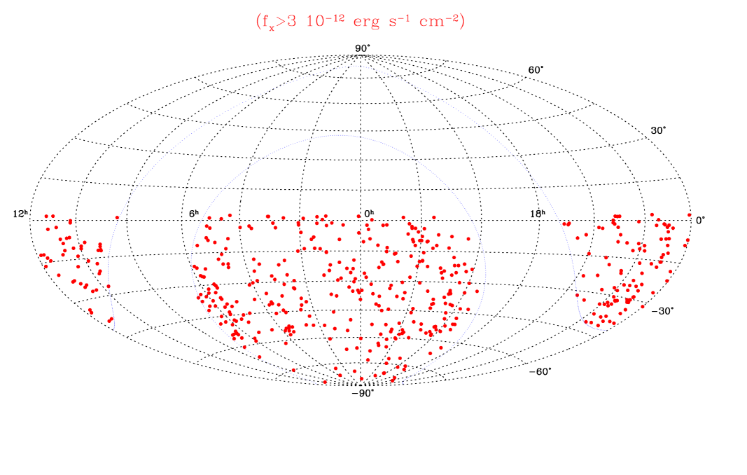
Figure 2: The distribution on the sky of the clusters in the REFLEX sample with $f_{x}>3\times 10^{-12}$ erg s^-1 cm^-2. Note that the area around the Magellanic Clouds ($\alpha\sim 1^{h}$ and $\sim 5^{h}$, $\delta\sim-70^{\circ}$), is not included in the survey.

Presently, we have selected a complete sample of 460 clusters to a nominal flux limit of $3\times 10^{-12}$ erg s^-1 cm^-2 (in the ROSAT band, 0.1–2.4 keV). Due to to the varying RASS exposure time and interstellar absorption over the sky, when a simultaneous requirement of a minimum number of source counts is applied, some parts of the sky may reach a lower flux. For example, when computing the preliminary REFLEX luminosity function presented in Böhringer et al (1998), a threshold of 30 source counts in the ROSAT hard band was set, which resulted in a slightly reduced flux limit over 21.5% of the survey area. The important point to be made is that a full map of these variations is known as a function of angular position and is exactly accounted for in all the statistical analyses.

This first sample, upon which the discussion on clustering and large-scale structure presented here is based, has been constructed to be at least 90% complete, as described in Böhringer et al. (1998). Several external checks, as comparisons with independently extracted sets of clusters, support this figure. The careful reader may have noticed that the total number of objects in this sample has been reduced by 15 since the time of writing our previous Messenger report. This is the result of the ongoing process of final identification and redshift measurement: spectroscopy and detailed deblending of X-ray sources have led to a reclassification of 15 X-ray sources which either had AGN counterparts or fell below the flux limit. With these new numbers, as of today 95% of the 460 candidates in this sample are confirmed and observed spectroscopically. Final clearing up and measurement of redshifts for the remaining $\sim 20$ candidates is foreseen for a forthcoming observing run next May. In the following, we shall simply refer to this complete sample as the “REFLEX sample”. The distribution on the sky of the REFLEX clusters defined in this way is shown in Figure 2.

3 Optical Follow-up Observing Strategy

The follow–up optical observations of REFLEX clusters were started at ESO in 1992, under the status of a Key Programme. The goal of these observations was twofold: a) obtain a definitive identification of ambiguous candidates; b) obtain a measurement of the mean cluster redshift.

First, a number of candidate clusters required direct CCD imaging and/or spectroscopy to be safely included in the sample.

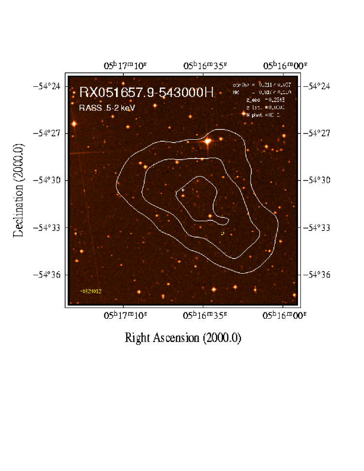
Figure 3: $15\times 15$ arcmin identification image of a REFLEX cluster at z=0.294. The optical image is from the Digitised Sky Survey (DSS), with superimposed the X–ray contours from the RASS. As suggested by the contours, this X-ray source shows a statistically significant extention.

For example, candidates characterised by a poor appearance on the Sky Survey IIIa-J plates, with no dominant central galaxy or featuring a point–like X–ray emission had to pass further investigation. In this case, either the object at the X-ray peak was studied spectroscopically, or a short CCD image plus a spectrum of the 2–3 objects nearest to the peak of the X-ray emission was taken. This operation was preferentially scheduled for the two smaller telescopes (1.5 m and 2.2 m, see below), and was necessary to be fully sure of keeping the completeness of the selected sample close to the desired value of 90%. In this way, a number of AGN’s were discovered and rejected from the main list.

Once a cluster was identified, the main scope of the optical observations was then to secure a reliable redshift. The observing strategy was designed so as to compromise between the desire of having several redshifts per cluster, coping with the multiplexing limits of the available instrumentation, and the large number of clusters to be measured. Previous experience on a similar survey of EDCC clusters (Collins et al. 1995), had shown the importance of not relying on just one or two galaxies to measure the cluster redshift, especially for clusters without a dominant cD galaxy. EFOSC1 in MOS mode was a perfect instrument for getting quick redshift measurements for 10–15 galaxies at once, but only for systems that could reasonably fit within the small field of view of the instrument (5.2 arcmin in imaging with the Tektronics CCD #26, but less than 3 arcmin for spectroscopy in MOS mode, due to hardware/software limitations in the use of the MOS masks). This feature clearly made this combination useful only for clusters above z=0.1, i.e. where at least the core region could be accommodated within the available area.

The other important aspect of using such an instrumental set–up is that in several cases, after removal of background/foreground objects one is still left with 8-10 galaxy redshifts within the cluster, by which a first estimate of the cluster velocity dispersion can be attempted. This clearly represents further, extremely important information related to the cluster mass, especially when coupled to the X-ray luminosity available for all these objects.

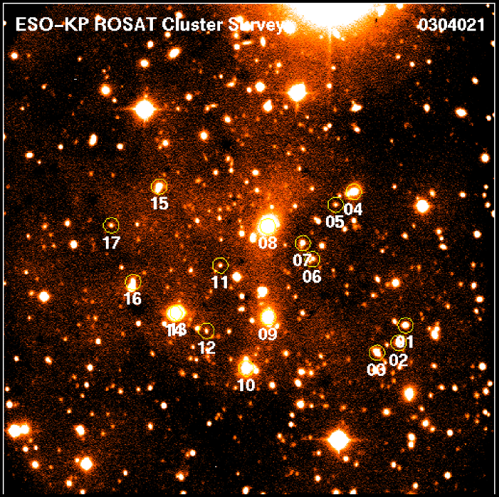
Figure 4: Short CCD exposure ($\sim 60$ sec) taken in white light with EFOSC1 at the 3.6 m telescope, covering the central region of the REFLEX cluster of previous figure. The field side is 5.2 arcmin. Note the remarkable glory of faint galaxies around the central brightest members. The numbers indicate the positions of the slitlets for the MOS observations.

At smaller redshifts, doing efficient multi–object spectroscopy work would have required a MOS spectrograph with a larger field of view, i.e. 20–30 arcminutes diameter. One possible choice could have been the fibre spectrograph Optopus (Avila et al. 1989), but its efficiency in terms of numbers of targets observable per night was too low for covering several hundred clusters as we had in our sample. The best solution in terms of telescope allocation pressure and performances was found in using single–slit spectroscopy and splitting the work between the 1.5 m and 2.2 m telescopes. Clearly, this required accepting some compromise in our wishes of having multiple redshifts, so that at the time of writing about 30% of the clusters observed at ESO have a measure based on less than 3 redshifts. The reliability of these as estimators of the cluster systemic velocity, however, is significantly enhanced by the coupling of the galaxy positions with the X–ray contours: we can clearly evaluate which galaxies have the highest probability to be cluster members. This is another advantage of a survey of X–ray clusters over optically–selected clusters. At the time of writing, in about seven years of work, we have observed spectroscopically a total of about 500 cluster candidates, collecting over 3200 galaxy spectra.

Figure 3 shows one example of the identification images, used for the first confirmation of the candidates. These pictures are constructed for all our candidates by combining the Digitised Sky Survey plates of the ESO/SRC atlas (image) and the RASS X–ray data (contours). Although this cluster (RX051657.9-543000), lies at a redshift z=0.294 (close to the redshift identification limit of REFLEX at z=0.32), a sufficient number of galaxies is detected in the optical image even at the depth of the survey plates. This picture gives a clear example of how the X–ray contours “guide the eye” in showing which are the “best” galaxies to be observed. In this case we had a MOS observation, but had we observed only the central two galaxies within the X–ray peak, we would have obtained a correct estimate of the cluster redshift.

The same cluster is then visible in the direct EFOSC1 image of Figure 4. This is a short service exposure (less than one minute), taken in white light as a template for the drilling of the slits on the EFOSC1 MOS mask. The image shows a spectacular abundance of faint galaxies, one of the most impressive cases observed during our survey.

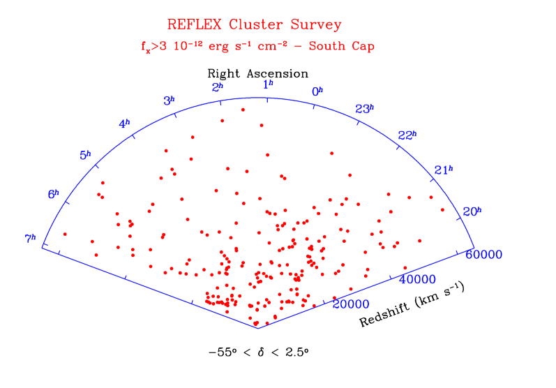
Figure 5: The large–scale distribution of REFLEX clusters within part of the South Galactic Cap region. Only objects North of $\delta=-55$ are shown, to avoid excessive confusion by the projection along declination.

After looking at this latest picture, it is natural to ask what is, for example, the galaxy luminosity function of this cluster, or what are the colours of this large population of faint objects. This is clearly important information, which at the moment, however, is only available for a restricted fraction of REFLEX clusters (Molinari et al. 1998). To cover this aspect, a wide–field imaging campaign is going to commence in the next semester, starting first with those medium–redshift clusters that best match the WFI at the 2.2 m telescope.

4 The Large–Scale Distribution of X–Ray Clusters

The cone diagram of Figure 5 plots the distribution of REFLEX clusters in the South Galactic cap area of the survey, selecting only objects with $z<0.2$ and $\delta>-55^{\circ}$, to ease visualization. One can easily notice a number of superstructures with sizes $\sim 100\rm\,h^{-1}\,Mpc$, that show explicitly the typical scales on which the cluster distribution is still inhomogeneous.

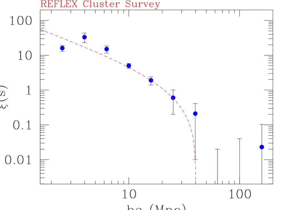
Figure 6: The two–point correlation function of clusters of galaxies in the REFLEX survey. The filled circles give the direct estimate, while the dashed line is computed by Fourier transforming the power spectrum of the survey data, that we showed in Böhringer 1998.

This inhomogeneity can be quantified at the simplest level through the two–point correlation function $\xi(s)$ , that measures the probability in excess of random of finding a pair of clusters with a given separation, (the variable $s$ is used here to indicate separations in redshift space). A preliminary estimate of $\xi(s)$ for the REFLEX sample is shown by the filled circles in Figure 6. The dashed line shows for comparison the Fourier transform of a simple fit to the power spectrum P(k), measured from a subsample of the same data (see Böhringer et al. 1998). The estimates of $\xi(s)$ and P(k) were performed by taking into account the angular dependence of the survey sensitivity, i.e., the exposure map of the ROSAT All-Sky Survey, and the NH map of galactic absorption. The good agreement between the two curves is on one side an indication of the self–consistency of the two estimators applied in redshift and Fourier space. Also, it shows a remarkable stability in the clustering properties of the sample, given that for the measure of P(k) the data were conservatively truncated at a comoving distance of $200\rm\,h^{-1}\,Mpc$ (Schuecker et al., in preparation), while the estimate of $\xi(s)$ uses the whole catalogue (Collins et al., in preparation). On the other hand, this also indicates that the bulk of the clustering signal on $\xi(s)$ is produced within the inner $200\rm\,h^{-1}\,Mpc$ of the survey, which is expected because this is the most densely sampled part of the flux–limited sample. We shall explore this in more detail when studying volume–limited samples, with a well–defined lower threshold in X-ray luminosity.

Figure 6 shows that $\xi(s)$ for clusters of galaxies is fairly well described by a power law out to $~{}40\rm\,h^{-1}\,Mpc$, and then breaks down, crossing the zero value around $50\rm\,h^{-1}\,Mpc$. It is interesting to compare it with the two–point correlation function of galaxies, as we do in Figure 7. The galaxy data shown here (points), are obtained from two volume–limited subsamples of the ESP survey (Guzzo et al. 1999). They are compared to $\xi(s)$ from the REFLEX clusters, given by the dashed lines. To ease the comparison, we preferred to plot the curves of $\xi(s)$ as computed from the Fourier transform of P(k). This is given by the top line, while the bottom line has been re–scaled by a factor $b_{c}^{2}=(3.3)^{2}$ in amplitude. This difference in amplitude, or bias, is expected, as clusters represent the high, rare peaks of the galaxy density distribution, and it can be demonstrated (Kaiser 1984), that their clustering has to be enhanced with respect to that of the general field. This quoted value of $b_{c}$, however, does not have a direct physical interpretation, as it is obtained from a flux–limited sample, and thus related to clusters having different mean intrinsic luminosities at different distances. One important aspect of selecting clusters through their X–ray emission is in fact that a selection in X-ray luminosity is closer to a selection in mass, than if one used a measure like the cluster richness (i.e. the number of galaxies within a given radius and a given magnitude range, as in the case of the Abell catalogue). For this reason, the observation that $\xi(s)$ has a different amplitude for volume–limited subsamples with different X–ray luminosity limits (i.e. a different value of $b_{c}$), has important implications for the theory (Mo & White 1996). The validity of a simple biasing amplification mechanism on these scales is explicitly supported by the very similar slopes of $\xi(s)$ shown in Figure 7 by galaxies and clusters. A full discussion concerning the luminosity dependence of the amplitude of the correlation function is being prepared (Collins et al., in preparation).

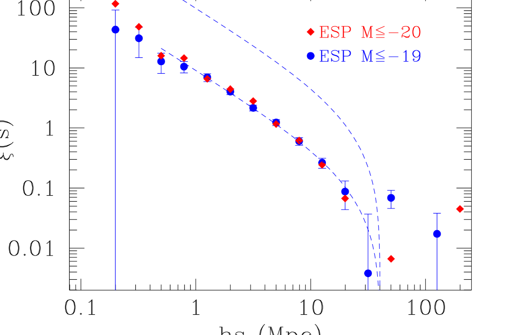
Figure 7: Comparison of the two–point correlation function of REFLEX clusters (top dashed line), to that of ESP galaxies (dots, Guzzo et al. 1999). The bottom dashed line is the REFLEX $\xi(s)$ after scaling by an arbitrary bias factor of $b_{c}^{2}=(3.3)^{2}$. The agreement in shape between galaxies and clusters is remarkable.

5 Conclusions

We have discussed how after several years of work with the X-ray data from the RASS and with ESO telescopes, the REFLEX project has reached a stage where the first significant results on large–scale structure can be harvested. We hope to have at least given a hint of how the REFLEX survey is possibly the first X-ray selected cluster survey where the highest priority was given to the statistically homogeneous sampling over very large solid angles. This makes it an optimal sample for detecting and quantifying the spatial distribution of the most massive structures in the Universe, as can be appreciated from the high S/N superclusters visible in the cone diagram of Figure 5 out to at least $z\sim 0.1$.

We have also shown how these results have been reached without specially designed instrumentation. Started in May 1992, with the next May run it will be seven years that we have been observing and measuring redshifts for REFLEX clusters. Again, this long timescale is a consequence of the fact that the project is based on “public” instrumentation, and therefore subject to the share of telescope time with the general ESO community. Clearly, even in these terms, this could have never been possible at ESO without the long–term “Key Programme” scheme. In fact it is exactly for surveys like REFLEX, i.e. large cosmology projects, that the concept of Key Programmes was originally conceived, under suggestion of those few people that at the end of the eighties were starting doing large–scale structure work in continental Europe. If the aim of the Key Programmes was that of making the exploration of the large-scale structure of the Universe feasible for European astronomers, providing them with a way to compete with the dedicated instrumentation of other institutions, we can certainly say that, after ten years, this major goal has probably been reached.

We thank Harvey MacGillivray and Paolo Vettolani for their support to the birth of this project and all the people who have contributed in different ways to its realization.

References

- [] Avila, G., D’Odorico, S., Tarenghi, M., & Guzzo, L., 1989, The Messenger, 55, 62
- [] Böhringer, H., et al., 1998, The Messenger, 94, 21 (astro-ph/9809382)
- [] Chincarini, G., & Guzzo, L., 1998, in Proc. of V-eme Colloque de Cosmologie, H. De Vega ed., in press
- [] Colless, M., 1998, Phil. Trans. R. Soc. Lond. A, in press (astro-ph/9804079)
- [] Collins. C.A., Guzzo, L., Nichol, R.C., & Lumsden, S.L., 1995, MNRAS, 274, 1071
- [] Da Costa, L.N., 1998, in Evolution of Large–Scale Structure: from Recombination to Garching, T. Banday & R. Sheth eds., in press (astro-ph/9812258)
- [] De Grandi, S., et al., 1999, ApJ (Letters), in press (astro-ph/9812423)
- [] Geller, M.J. & Huchra, J.P., 1989, Science, 246, 897
- [] Guzzo, L., 1999, in Proc. of XIX Texas Symposium, (Paris - October 1998), Elsevier, in press
- [] Guzzo, L., et al. (The ESP Team), 1999, A&A, in press (astro-ph/9901378)
- [] Kaiser, N., 1984, ApJ, 284, L9
- [] Margon, B., 1998, Phil. Trans. R. Soc. Lond. A, in press (astro-ph/9805314)
- [] Mo, H.J., & White, S.D.M., 1996, MNRAS, 282, 347
- [] Molinari, E., Moretti, A., Chincarini, G., & De Grandi, S., 1998, A&A, 338, 874
- [] Schuecker, P., Ott, H.-A., & Seitter, W.C., 1996, ApJ, 472, 485
- [] Shectman, S.A., et al., 1996, ApJ, 470, 172
- [] Vettolani, et al. (the ESP Team), 1998, A&AS, 130, 323