The Radiative Feedback of the First Cosmological Objects

Abstract

In hierarchical models of structure formation, an early cosmic UV background (UVB) is produced by the small ($T_{\rm vir}\;\hbox to0.0pt{\lower 2.5pt\hbox{$\sim$}\hss}\raise 1.5pt\hbox{$<$}\;10^{4}$K) halos that collapse before reionization. The UVB at energies below 13.6eV suppresses the formation of stars or black holes inside small halos, by photo–dissociating their only cooling agent, molecular ${\rm H_{2}}$. We self–consistently compute the buildup of the early UVB in Press–Schechter models, coupled with ${\rm H_{2}}$ photo–dissociation both in the intergalactic medium (IGM), and inside virialized halos. We find that the intergalactic ${\rm H_{2}}$ has a negligible effect on the UVB, both because its initial optical depth is small ($\;\hbox to0.0pt{\lower 2.5pt\hbox{$\sim$}\hss}\raise 1.5pt\hbox{$<$}\;0.1$), and because it is photo–dissociated at an early stage. If the UV sources in the first collapsed halos are stars, then their UV flux suppresses further star–formation inside small halos. This results in a pause in the buildup of the UVB, and reionization is delayed until larger halos ($T_{\rm vir}\;\hbox to0.0pt{\lower 2.5pt\hbox{$\sim$}\hss}\raise 1.5pt\hbox{$>$}\;10^{4}$K) collapse. If the small halos host mini–quasars with hard spectra extending to $\sim$1keV, then their X–rays balance the effects of the UVB, the negative feedback does not occur, and reionization can be caused by the small halos.

FERMILAB-Pub-99/041-A

1. Introduction

Recent progress in high redshift observations has made it possible to estimate the global star–formation history of the universe to redshifts as high as $z\sim 5$. Although the evolution of the star–formation rate (SFR) is relatively well–established at lower redshifts ($z\;\hbox to0.0pt{\lower 2.5pt\hbox{$\sim$}\hss}\raise 1.5pt\hbox{$<$}\;2$), there is still substantial uncertainty about the $2\;\hbox to0.0pt{\lower 2.5pt\hbox{$\sim$}\hss}\raise 1.5pt\hbox{$<$}\;z\;\hbox to0.0pt{\lower 2.5pt\hbox{$\sim$}\hss}\raise 1.5pt\hbox{$<$}\;5$ era. A study of Lyman break galaxies in the Hubble Deep Field shows a decline of the SFR towards high $z$, indicating a peak in the SFR around $z\sim 2$ (Madau et al. 1996). On the other hand, a recent census of $z\;\hbox to0.0pt{\lower 2.5pt\hbox{$\sim$}\hss}\raise 1.5pt\hbox{$>$}\;3$ galaxies, detected in Ly$\alpha$ emission in a $\sim 200$ times wider field, suggests that the SFR is either constant, or increasing from $z\sim 2$ to $z\sim 5$ (Steidel 1999). At present, these uncertainties render extrapolations of the observed SFR to still higher ($z\;\hbox to0.0pt{\lower 2.5pt\hbox{$\sim$}\hss}\raise 1.5pt\hbox{$>$}\;5$) redshifts unreliable.

We do know, however, that some stellar activity must have taken place at $z>5$. The presence of heavy elements observed in the high redshift Ly$\alpha$ forest (Tytler, Cowie), as well as the reionization of the intergalactic medium (IGM), require sources of metals and ionizing photons in addition to the currently known population of galaxies and quasars. Such ultra–high redshift objects are indeed expected in the current best–fit cosmological cold dark matter (CDM) models, which predict that the first virialized halos appear at redshifts as high as $z\sim 30$. It is natural to identify these small halos as the sites where the first stars or massive black holes are born, forming the first generation of ”mini–galaxies” or ”mini–quasars”.

The first collapsed halos have masses near the cosmological Jeans mass, $M\sim 10^{4-5}~{}{\rm M_{\odot}}$, implying a virial temperature of a few hundred K. In order to form either stars or black holes, the gas in these halos must be able to cool efficiently. At this low temperature, the only mechanism in the chemically simple primordial gas that satisfies this requirement is collisional excitations of ${\rm H_{2}}$ molecules. At still higher temperatures ($T\;\hbox to0.0pt{\lower 2.5pt\hbox{$\sim$}\hss}\raise 1.5pt\hbox{$>$}\;10^{4}$K) and masses ($M\sim 10^{8}~{}{\rm M_{\odot}}$), efficient cooling is enabled by atomic hydrogen. The presence or absence of ${\rm H_{2}}$ molecules in the first collapsed halos therefore determines whether these small halos can form any stars or quasars, before larger halos dominate the collapsed baryonic fraction. As a consequence, the ${\rm H_{2}}$ abundance determines when the ”dark age” ends: if there is sufficient ${\rm H_{2}}$ inside the first small halos, the dark age ends earlier; if ${\rm H_{2}}$ is absent, it ends at the later redshift when the larger scales collapse.

The fraction of ${\rm H_{2}}$ molecules in the post–recombination IGM is $x_{\rm H_{2}}\equiv n_{\rm H2}/n_{\rm H}\sim 10^{-6}$. In the absence of a background radiation field, this fraction rises to $\sim 10^{-4}$ at the dense central regions of collapsed halos (Haiman et al. 1996; Tegmark et al. 1997), high enough to satisfy the cooling criterion. However, ${\rm H_{2}}$ molecules are fragile, and are photo-dissociated efficiently by a low–intensity UV radiation. In a previous paper (Haiman et al. 1997, hereafter HRL97), we showed that the flux necessary for ${\rm H_{2}}$ photo–dissociation is several orders of magnitude smaller than the flux needed to reionize the universe. Based on this result, we conjectured that the ${\rm H_{2}}$ abundance in the first collapsed halos was suppressed soon after a small number of these halos formed stars or turned into mini–quasars.

This negative feedback would imply that the bulk of the first mini–galaxies or mini–quasars would reside in dark halos with masses at least $10^{7-8}~{}{\rm M_{\odot}}$, and that the ”dark age” would end only at the typical collapse redshift of these halos. The first condensations at the $\sim 1000$ times smaller Jeans mass would then remain neutral, gravitationally confined gas clumps, until they merge into larger systems, or are photo–evaporated by the UVB established after reionization (Barkana & Loeb 1998). A small fraction of these clumps is expected to survive mergers and photo–evaporation until $z\sim 3$; based on their column density and abundance, Abel & Mo (1998) have identified this survived fraction with the Lyman limit systems observed near $z\sim 3$. A direct observational study of the first collapsed halos will be feasible in the future with the Next Generation Space Telescope (NGST): with its $\sim 1$nJy imaging sensitivity, NGST will be able to detect a $\sim 10^{6}~{}{\rm M_{\odot}}$ halo with an average star formation efficiency at $z\sim 10$ (Smith & Koratkar 1998).

In this paper, we study the conjecture of HRL97 in a cosmological setting, by quantifying the radiative feedback of the first collapsed halos on their ${\rm H_{2}}$ abundance, as the early UVB is established in Press–Schechter models. The two main questions we address are: (1) How does the ${\rm H_{2}}$ feedback effect the typical masses and collapse redshifts of the first halos; and (2) Could the first collapsed dark halos, with masses near the Jeans mass, contribute to the early UVB, and to the reionization of the universe?

In HRL97, we concluded that the negative feedback suppresses the fragmentation and collapse of small halos. In the present paper, we confirm this basic conclusion, although we find that it depends sensitively on the spectrum of the early sources. Our calculations improve HRL97 in several ways. We solve the coupled evolution of the formation of new halos (using the Press–Schechter formalism), the build–up of the early UVB, and the evolution of the ${\rm H_{2}}$ abundance in the IGM and inside each collapsed halo; we explore the sensitivity of our conclusions on the spectral shape, specifically the X–ray to UV flux ratio; we replace our assumption of homogeneous slabs by the centrally condensed profiles expected for virialized halos; and we employ a more realistic star–formation criterion.

This paper is organized as follows. In § 2, we quantify the spectrum of the early UVB after processing through the intergalactic H and ${\rm H_{2}}$. In § 3, we compute the ${\rm H_{2}}$ abundance in virialized halos under this UVB, and define our criterion for star–formation. In § 4, we compute the evolution of the UVB coupled with the ${\rm H_{2}}$–feedback, and present these results in § 5. In § 6, we discuss how these results are modified in the presence of early mini–quasars with spectra extending to the X–rays. Finally, § 7 summarizes the main conclusions and implications of this work.

Throughout this paper, we adopt a background $\Lambda$CDM cosmology with a tilted power spectrum, $(\Omega_{0},\Omega_{\Lambda},\Omega_{\rm b},h,\sigma_{8h^{-1}},n)=(0.35,0.65,0.04,0.65,0.87,0.96)$; however, our results are relevant in any model where the cosmic structure is built hierarchically from the “bottom up”. For convenience, we also adopt the following terminology: a ”small halo” is defined to be a halo with virial temperature $T\;\hbox to0.0pt{\lower 2.5pt\hbox{$\sim$}\hss}\raise 1.5pt\hbox{$<$}\;10^{4}$K, or equivalently, with mass $M\;\hbox to0.0pt{\lower 2.5pt\hbox{$\sim$}\hss}\raise 1.5pt\hbox{$<$}\;3\times 10^{7}~{}{\rm M_{\odot}}[(1+z)/11]^{-3/2}$. Conversely, a ”large halo” is defined as a halo with virial temperature $T\;\hbox to0.0pt{\lower 2.5pt\hbox{$\sim$}\hss}\raise 1.5pt\hbox{$>$}\;10^{4}$K, or equivalently, with mass $M\;\hbox to0.0pt{\lower 2.5pt\hbox{$\sim$}\hss}\raise 1.5pt\hbox{$>$}\;3\times 10^{7}~{}{\rm M_{\odot}}[(1+z)/11]^{-3/2}$.

2. Radiative Transfer of the Soft UV Background

In hierarchical models of structure formation, small objects appear at high redshift, and larger objects form later, with the total fraction of collapsed baryons monotonically increasing with time. The radiation output associated with the collapsed halos gradually builds up a cosmic UV background. Of interest here is the background in the 11.18–13.6 eV range, enclosing the Lyman and Werner (LW) bands of molecular ${\rm H_{2}}$. Photons in this range do not ionize neutral H atoms, and can travel to a large fraction of the Hubble length across the IGM, and photo–dissociate molecular ${\rm H_{2}}$ both in the IGM and inside other collapsed halos. Since the presence of ${\rm H_{2}}$ is a necessary condition for the formation of stars or a central black hole, this leads to a feedback that controls the fraction of collapsed baryons turned into luminous sources, and the evolution of the UVB. Before addressing the feedback itself, in this section we quantify the spectral shape of the UVB in the relevant frequency range. This is determined by the absorption of the flux by intergalactic H and ${\rm H_{2}}$.

2.1. ”Sawtooth” Modulation From Neutral H

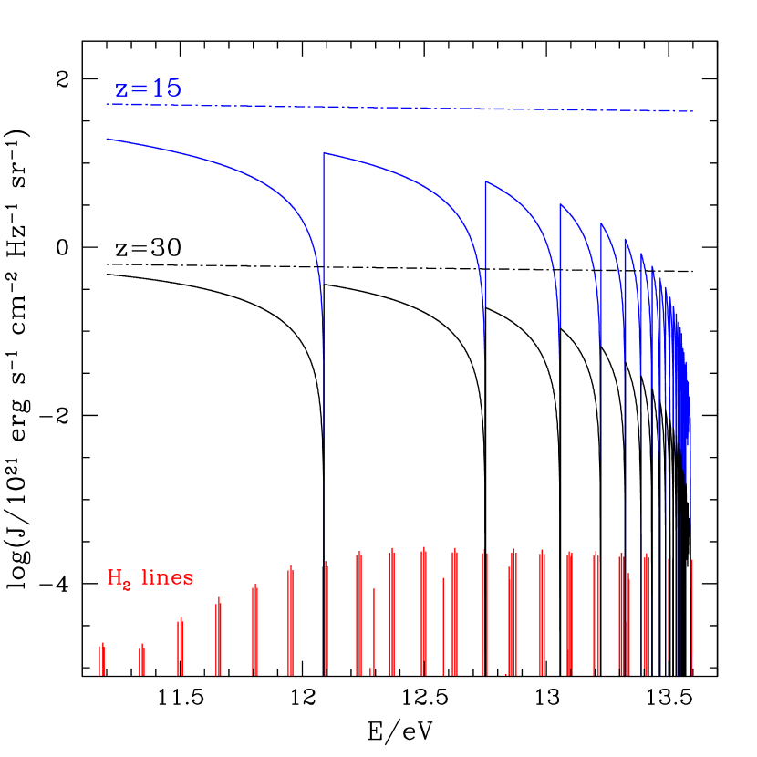
Figure 1.— The spectrum of the UV background at redshifts $z=30$ and $z=15$ in the cosmological model of Figure 7. The solid lines show the spectrum after absorption by neutral H in the high–redshift IGM; the dashed lines show the spectrum without this absorption. For reference, at the bottom of the figure we show the location of the 76 LW lines of ${\rm H_{2}}$. The length of each line indicates its relative contribution to ${\rm H_{2}}$ dissociations (see the Appendix and Figure 16 for the numerical values of the dissociation fractions and oscillator strengths.

Consider an observer at redshift $z_{\rm obs}$, measuring the UVB at the local frequency $\nu_{\rm obs}$, where $11.18{\rm eV}<h\nu_{\rm obs}<13.6{\rm eV}$. The photons collected at the frequency $\nu_{\rm obs}$ are arriving from sources located at $z_{\rm s}>z_{\rm obs}$, and have redshifted their original frequency $\nu_{\rm s}>\nu_{\rm obs}$ to $\nu_{\rm obs}$. If during its travel, the photon’s frequency equals the frequency of any atomic Lyman line, it is absorbed by the neutral IGM, because the optical depth of the IGM in these lines are exceedingly high, e.g. $\tau_{\rm Ly\alpha}\sim 10^{6}$ at $z\sim 20$. This statement applies to all Lyman lines with $2<n\;\hbox to0.0pt{\lower 2.5pt\hbox{$\sim$}\hss}\raise 1.5pt\hbox{$<$}\;150$. The Ly$\alpha$ absorption ($n=1$) has only a small effect on the background, since most of the absorbed photons are simply re-emitted at the same frequency, except those converted to lower frequency photons by two–photon decays. In any case, the Ly$\alpha$ resonance is at 10.2 eV, outside the frequency range of interest here. The very high Lyman lines ($n\;\hbox to0.0pt{\lower 2.5pt\hbox{$\sim$}\hss}\raise 1.5pt\hbox{$>$}\;150$) have small enough cross–sections so that the total optical depth of the IGM at these frequencies drops below unity. However, these resonances have a negligible contribution to the total absorption in the 11.8-13.6eV range. Here we make the simple assumption that a ”dark screen” blocks the view of all sources at redshifts above $z_{\rm max}$. The maximum redshift is given by

$$\frac{1+z_{\rm max}}{1+z_{\rm obs}}=\frac{\nu_{\rm i}}{\nu_{\rm obs}},$$ (1)

where $\nu_{\rm i}$ is the frequency of the Lyman line closest from above to the observed frequency, $\nu_{\rm obs}$.

The processing of the early UVB by the neutral IGM leads to a characteristic spectral shape, resembling a ”sawtooth”, since the closer $\nu_{\rm obs}$ is to a resonance, the nearer the screen is to the observer. The resulting spectrum is shown in a specific model (described below) in Figure 1. The redshift distribution of sources is important for the magnitude of this “sawtoothing” effect. If a large fraction of the sources contributing to the UVB are located near the observer, then the effect is smaller; if the sources are spread out over a wider range of redshifts, then the effect is larger. In the hierarchical models, new halos form exponentially rapidly at high redshifts. At any given time, most of the sources are expected to have formed recently, i.e. at redshifts only slightly above that of the observer. Since the formation rate of new halos decreases with redshifts, the sawtoothing will be increasingly pronounced at later times. This is illustrated in Figure 1: the flux is suppressed by a larger average factor at $z=15$ than it is at $z=30$.

2.2. Modulation From ${\rm\bf H_{2}}$ Molecules

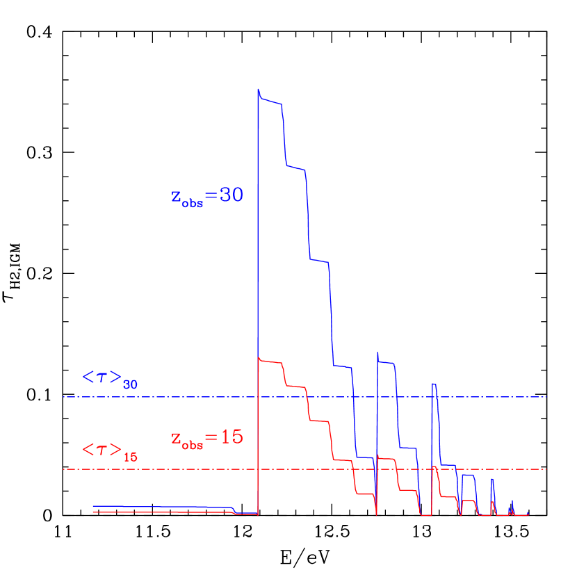
Figure 2.— The total ${\rm H_{2}}$ optical depth of the IGM for an observer at redshift $z=30$ and $z=15$. We assume a constant fixed $x_{\rm H_{2}}=2\times 10^{-6}$, and sum the optical depth of the Lyman-Werner lines of ${\rm H_{2}}$. At each observed frequency, we only include sources between $z_{\rm obs}$ and the nearest atomic Lyman resonance. The dashed lines show the effective optical depths averaged in the 11.18–13.6eV range.

In addition to absorption by neutral H, the UVB may also be modulated by the intergalactic ${\rm H_{2}}$. The ${\rm H_{2}}$ in the IGM removes photons from the UVB when these molecules are photo–dissociated, and decreases the rate of photo–dissociations inside collapsed halos. It is important, therefore, to assess the magnitude of the modulation from the intergalactic ${\rm H_{2}}$.

When a LW photon is absorbed by an ${\rm H_{2}}$ molecule, there is on average a $\sim 15$% chance that it causes a photo–dissociation of the molecule. This is the average probability that the molecule decays from its excited state to a continuum of two distinct H atoms (Solomon, cf. Field et al. 1966; Stecher & Williams 1967). We will assume here that in the other $\sim 85\%$ of absorptions, the LW photons is re-emitted at the same frequency, and there is no net effect. This is justified because the quadrupole transitions among the excited electronic states are much slower than decay back to the electronic ground state, and also because the small dipole moment that preferred the upper state in the absorption will preferentially populate the initial lower state in the decay (Herzberg 1950).

If the ${\rm H_{2}}$ fraction in the IGM is $x_{\rm H_{2}}=n_{\rm H_{2}}/n_{\rm H}$, then the total optical depth of the IGM at redshift $z$ and frequency $\nu$ to ${\rm H_{2}}$–dissociations is given by

$$\tau_{\rm H_{2}}(\nu,z)=x_{\rm H_{2}}\frac{\pi e^{2}}{m_{\rm e}c}\sum_{i=1}^{76}f_{\rm diss,i}f_{\rm osc,i}\int_{z}dz^{\prime}c\frac{dt}{dz^{\prime}}n_{\rm H}(z^{\prime})\phi(\nu_{z^{\prime}},\nu_{\rm i}),$$ (2)

where the sum is over the 76 LW lines of ${\rm H_{2}}$; $n_{H}=8.5\times 10^{-6}\Omega_{\rm b}h^{2}(1+z)^{3}$ is the neutral H number density in the IGM; $f_{\rm diss,i}$ is the probability that absorption into the ${\rm i^{th}}$ LW line is followed by a dissociative decay; $f_{\rm osc,i}$ is the oscillator strength of the ${\rm i^{th}}$ LW line; $\nu_{z^{\prime}}\equiv\nu(1+z^{\prime})/(1+z)$; $cdt/dz$ is the line element in our $\Lambda$CDM cosmology; and $\phi(\nu,\nu_{\rm i})$ is the absorption line profile centered around the resonance frequency $\nu_{\rm i}$. We included the equilibrium ortho to para ratio of 3:1 of H₂ implicitly in equation (2) by appropriately multiplying the oscillator strengths with 0.75 or 0.25 respectively. Furthermore, we assume that the line shapes follow a Voigt profile with thermal broadening by the IGM temperature (taken to be $T=0.0135(1+z)^{2}$ K, although the total optical depth, and therefore our results, are insensitive to this choice). More information on the details of H₂ pre–dissociation are given in the Appendix.

Equation 2 gives a formal sum total optical depth of the 76 LW resonances, each of which is at a different frequency. From the point of view of a photon traveling across the IGM, these resonances would be encountered at different redshifts. During its lifetime, a UV photon can therefore be subjected only to a subset of the LW resonances: as we argued in § 2.1 above, the maximum redshift interval a UV photon can travel before it is absorbed by a neutral H atom corresponds to the redshift between two neutral H resonances. A simple calculation of the optical depth using equation 2 would result in an overestimate by a factor of a few (depending on $z$ and $\nu$) of the true value relevant to the observed modulation of the UVB. To impose the fact that the UVB is simultaneously modulated both by the intergalactic H and ${\rm H_{2}}$, one needs to change the summation in Equation 2 from $i\in$(1,76) to $i\in$($i_{\rm min}$,$i_{\rm max}$), where $i_{\rm min}$ is the LW resonance closest in frequency from above to $\nu$, and $i_{\rm max}$ is the LW resonance farthest above $\nu$ before encountering an atomic Lyman line (see Figure 1 and Figure 16 for visualizations of the relative location of the H and ${\rm H_{2}}$ lines).

In Figure 2, we show the resulting optical depth as a function of the observed frequency, for two different redshifts, $z=15$ and $z=30$. As the figure shows, the optical depth is largest at $\sim$12.1eV. This is because the largest frequency gap between the atomic lines occurs between Ly$\beta$ and Ly$\gamma$, enclosing the largest subset of the ${\rm H_{2}}$ LW lines with significant contributions to ${\rm H_{2}}$ dissociations (see Figures 1 and 16). Figure  2 also shows that the maximum optical depth is 0.35 and 0.13 for $z=30$ and $z=15$, respectively (assuming $x_{\rm H_{2}}=2\times 10^{-6}$). Interestingly, the characteristic features in Figure 2 depend only on the relative frequencies of atomic vs. molecular resonant absorption lines (shown in Figure 16), i.e. only on atomic and molecular physics.

The total optical depths are near, but somewhat below unity. This result has several consequences. It is useful here to draw an analogy with the ionization of neutral H. The total optical depth of the IGM to H photo–ionizations (just above 13.6eV) is $\tau_{\rm H}\sim 100[(1+z)/21]^{3}$, which justifies the simple picture of isolated HII regions (”Strömgren spheres”), each bounded by a sharp ionization front, and continuously expanding around each ionizing source. The situation with ${\rm H_{2}}$ is different in two ways: the optical depth is less than unity, and is distributed among several LW lines, each of which is individually optically thin, and causes dissociations at a different redshift relative to each source. As a consequence, no sharp ${\rm H_{2}}$ dissociation “front” exists.

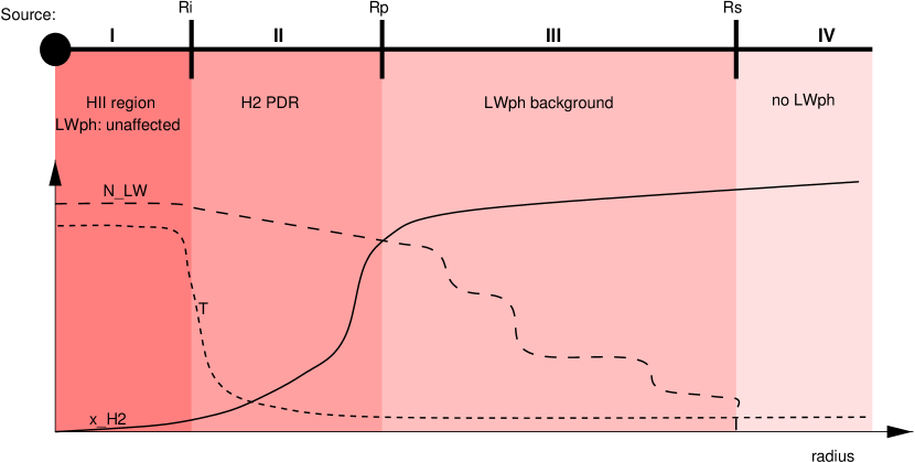
Figure 3.— Schematic sketch of the radial structure of a cosmological photo–dissociation region. Region I is the usual Strömgren sphere, bounded by the H I ionization front at $R_{\rm i}$. Inside this region, the temperature is high ($\sim 10^{4}$K) hydrogen is ionized, and the H₂ abundance tends to zero. Region II extends from $R_{\rm i}$ to the radius $R_{\rm p}$ where the H₂ photodissociation time becomes longer than the Hubble time. Here the temperature is that of the IGM, the H₂ fractions are still low, but slowly rise to the background value of $\sim 2\times 10^{-6}$. Region III extends from $R_{\rm p}$ to the radius $R_{\rm s}$, where Ly$\gamma$ shifts to Lyman$\beta$. In this region, the source contributes to the soft UV background, but its flux is diminished by absorption into the atomic Lyman series. In region IV beyond $R_{\rm s}$, all photons in the Lyman Werner bands are absorbed by an atomic Lyman line. Hence, at such large scales, an individual source does not contribute to the UVB and intergalactic H₂ dissociation. See § 2.2 for a more detailed discussion.

A schematic sketch of four distinct regions in the radial structure of an ${\rm H_{2}}$ photo–dissociation region is shown in Figure 3. Region I extends to the usual H I ionization front or Strömgren radius. Inside this region, the temperature is high ($\sim 10^{4}$K), hydrogen is ionized, H₂ is photo–dissociated, and the H₂ abundance tends to zero. Region II is defined to extend from $R_{\rm i}$ to the radius $R_{\rm p}\sim 2.5\,h^{-1/2}(1+z)_{30}^{-3/4}N_{LW,47}^{1/2}\;\;{\rm kpc}$, where the H₂ photodissociation time becomes longer than the Hubble time. Here $N_{LW,47}=N_{LW}/10^{47}{\rm s}^{-1}$ is the photon number flux in the Lyman Werner bands per second. In this region the temperature is that of the IGM, and the H₂ fractions are still low, but slowly rise to its background value of $\sim 2\times 10^{-6}$. Since the optical depth in the Lyman Werner lines are very small, the dissociation front is significantly diluted. Region III is defined to extend from $R_{\rm p}$ to the radius $R_{\rm s}\approx 2h^{-1}[(1+z)/31]^{-1.5}~{}{\rm Mpc}$ where Lyman $\gamma$ shifts to Lyman$\beta$. In this region, the source contributes to the soft UV background, but its flux is diminished by absorption into the atomic Lyman series. In region IV beyond $R_{\rm s}$, all photons in the Lyman Werner bands are absorbed by an atomic Lyman line. Hence, at such large scales, an individual source does not contribute to the UVB and intergalactic H₂ dissociation.

Although the maximum optical depths from the intergalactic ${\rm H_{2}}$ are relatively small, the UVB flux can be suppressed by as much as $1-\exp(-0.35)\sim 50$%. However, we are interested in the suppression of the ${\rm H_{2}}$ photo–dissociation rate when the UVB falls on a collapsed halo. This suppression is smaller than 50%, since the photo–dissociation rate is given by a weighted average of the observed flux in the 11.18–13.6eV range. We therefore define an “effective” optical depth $<\tau>_{z}$, that directly characterizes the suppression of the ${\rm H_{2}}$ photo–dissociation rate, as follows:

$$\begin{array}[]{l}k_{\rm diss,0}(z)=4\pi x_{\rm H_{2}}n_{\rm H}(z)\frac{\pi e^{2}}{m_{\rm e}c}\times\\ \mbox{ }\sum_{\rm i=i_{min}}^{\rm i_{max}}f_{\rm diss,i}f_{\rm osc,i}\int_{\nu}d\nu^{\prime}\phi(\nu^{\prime},\nu_{\rm i})\frac{J_{\nu^{\prime}}(z)}{h\nu^{\prime}},\end{array}$$ (3)

$$\begin{array}[]{l}k_{\rm diss}(z)=4\pi x_{\rm H_{2}}n_{\rm H}(z)\frac{\pi e^{2}}{m_{\rm e}c}\times\\ \sum_{\rm i=i_{min}}^{\rm i_{max}}f_{\rm diss,i}f_{\rm osc,i}\int_{\nu}d\nu^{\prime}\phi(\nu^{\prime},\nu_{\rm i})\frac{J_{\nu^{\prime}}(z)}{h\nu^{\prime}}\exp[-\tau_{\rm H_{2}}(\nu^{\prime},z)],\end{array}$$ (4)

$$<\tau>_{z}\equiv-\log[k_{\rm diss}(z)/k_{\rm diss,0}(z)].$$ (5)

Here $J_{\nu}(z)$ is the UVB flux before processing by the intergalactic ${\rm H_{2}}$, and $\tau_{\rm H_{2}}(\nu,z)$ is the optical depth at this frequency shown by the solid lines in Figure 2. When the sources are assumed to be distributed according to the Press–Schechter model (see below), the maximum reduction in the ${\rm H_{2}}$ photo–dissociation rate is 10% at $z=30$ and 4% at $z=15$ (see the dashed lines in Figure 2). Note, however, that these numbers assume a constant $x_{\rm H_{2}}=2\times 10^{-6}$. In reality (as will be shown below), the intergalactic ${\rm H_{2}}$ fraction drops sharply soon after the appearance of the first sources, before the UVB builds up to the level of causing any ${\rm H_{2}}$ feedback inside the collapsed clumps. This is because the ${\rm H_{2}}$ dissociation time in the IGM, $1/k_{\rm diss}$ becomes shorter than the Hubble time at $J\sim 10^{-3}$, while the feedback on the dense clumps typically turns on only later, when the UVB reaches $J\sim 10^{-2}$.

In summary, we have shown that the intergalactic ${\rm H_{2}}$ might cause a maximum of $\sim 50\%$ suppression of the UVB near 12 eV, but the overall effect on the ${\rm H_{2}}$ photo–dissociation rate is small: less than 10%, assuming a constant intergalactic ${\rm H_{2}}$ fraction of $2\times 10^{-6}$. We will show below that the intergalactic ${\rm H_{2}}$ fraction is substantially reduced, and therefore this small modulation disappears, by the redshifts of interest – when the UVB builds up to the levels to photo–dissociate ${\rm H_{2}}$ molecules in dense collapsed clumps.

3. ${\rm\bf H_{2}}$-Cooling in the Presence of the UV Background

In this section, we consider the behaviour of individual, centrally condensed gas clouds, when illuminated by an external UVB. Here, we assume the UVB to have a fixed amplitude, and postpone the treatment of the coupled evolution of the UVB, and the ${\rm H_{2}}$ abundance and star formation to § 4 below.

3.1. The ${\rm\bf H_{2}}$ Abundance in Collapsed Clouds

The radiative efficiency of a gas cloud by collisional excitations of ${\rm H_{2}}$ molecules depends on the gas temperature, density, and ${\rm H_{2}}$ abundance. Although the typical average overdensity of a virialized spherical perturbation is $\delta\sim 100-200$, in a centrally condensed cloud, the central density can reach a much higher value. This is important in the present context, because the formation of ${\rm H_{2}}$ molecules can be enhanced by the accelerated chemistry inside the central, dense regions. In addition, the total integrated column density of a centrally condensed cloud is higher than that of a homogeneous sphere with the same mass and density. Central condensation therefore tends to make the clouds more self–shielding against the external UVB, and help to preserve the internal ${\rm H_{2}}$ molecules.

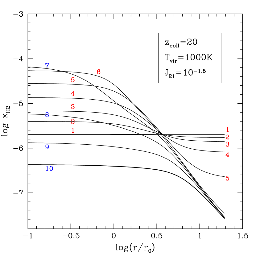
Figure 4.— The time–evolution of the ${\rm H_{2}}$ profile in a truncated isothermal sphere in the presence of an external flux. The example shown is for a truncated singular isothermal sphere with $T_{\rm vir}=10^{3}$K, $z_{\rm coll}=20$, and $J_{21}=10^{-1.5}$. Increasing numbers correspond to equal time–steps in logarithmic time, upto a Hubble time of $\sim 5\times 10^{15}$ sec. At the outskirts of the cloud the H₂ fraction decreases with time. In the core molecules are formed initially via $H^{-}\ +\ H\ \rightarrow\ H_{2}\ +\ e^{-}$ at a rate exceeding the photo–dissociation rate. At the point where the electron fraction drops below $10^{-5}$ photo–dissociation becomes dominant and H₂ is destroyed in the already self–shielding core.

To characterize the central condensation, here we adopt the density profiles of truncated isothermal spheres (TIS, Shapiro et al. 1999). These profiles are especially convenient, since they have a one–to–one correspondence with the final virialized state of the spherical top–hats used in the Press–Schechter formalism. The spheres are isothermal at the virial temperature, their average overdensity is $\sim 130$, and their central overdensity in the core reaches $\sim 10^{4}$. The TIS profiles are similar to the spherically averaged universal profiles found in numerical simulation of clusters (NFW, Navarro et al. 1998). The main difference from NFW is that the TIS has a central core (the existence of cores are indicated by recent simulations of galaxy groups, e.g. by Kravtsov et al. 1998).

We assume that the TIS is composed of the nine species ${\rm H}$, ${\rm H^{-}}$, ${\rm H^{+}}$, ${\rm He}$, ${\rm He^{+}}$, ${\rm He^{++}}$, ${\rm H_{2}}$, ${\rm H_{2}^{+}}$, and ${\rm e^{-}}$, with the initial abundances given by their post–recombination values (Anninos and Norman 1996). Our results are insensitive to the precise initial conditions, such as the electron fraction (${\rm x_{e}\approx 10^{-4}}$) and molecule fraction ($x_{\rm H_{2}}\approx 2\times 10^{-6}$). Although these abundances represent the chemical composition of the IGM, and we start with a cloud that is already collapsed and virialized, this should not effect our final results. In 1–D spherical simulations (Haiman, Thoul & Loeb 1996), we have found that the abundances stay near their initial IGM values until the formation of the virialization shock; soon after virialization the abundances loose memory of their initial values.

We solve the subsequent time evolution of the chemical abundances, as a function of radius throughout the cloud, assuming that the cloud is illuminated by the external UVB. The UVB flux is assumed to be a power law below 13.6eV,

$$J_{\nu}=J_{21}\left(\frac{\nu}{\nu_{\rm H}}\right)^{-1}~{}\times{\rm sawtooth~{}}~{}~{}~{}~{}h\nu<13.6{\rm eV},$$ (6)

and to be zero above 13.6eV, since the flux from stellar sources would suppressed by several orders of magnitude by the neutral IGM. The sawtooth modulation by the intergalactic H is described above, and the constant amplitude $J_{21}$ is in units of $10^{-21}~{}~{}{\rm erg~{}s^{-1}~{}cm^{-2}~{}Hz^{-1}~{}sr^{-1}}$. Our results are insensitive to the shape of the UVB, since we only utilize the flux between 11.18 and 13.6 eV. The possibility of a non–stellar flux, extending to higher energies will be discussed in section § 6 below. The chemical reaction rates and cross–sections are taken from Haiman, Thoul & Loeb (1996). We have solved the radiative transfer across the cloud, assuming spherical symmetry, and included the self–shielding due to both H and ${\rm H_{2}}$. The initial conditions are specified by the virial temperature $T_{\rm vir}$, and collapse redshift $z_{\rm coll}$ of the TIS, and the amplitude of the UVB, $J_{21}$.

An illustrative example of the evolution of the ${\rm H_{2}}$ abundance is shown in Figures 4 and 5. Figure 4 shows the radial profile of $x_{\rm H_{2}}$ at 10 different time–steps, equally spaced in logarithmic time, during a time–interval that corresponds to the Hubble time at $z=20$, $t\approx 5\times 10^{15}$ sec. The cloud is assumed to be a TIS with $z_{\rm coll}=20$ and $T_{\rm vir}=10^{3}$K, and the amplitude of the UVB is taken to be $J_{21}=10^{-1.5}$. As Figure 4 shows, initially the ${\rm H_{2}}$ fraction rises in the core: this is because new ${\rm H_{2}}$ molecules form via the charge transfer reactions ${\rm H+e^{-}\rightarrow H^{-}+\gamma}$ and ${\rm H^{-}+H\rightarrow H_{2}+e^{-}}$, utilizing the initial residual free electrons. By $t=10^{14}$ sec, $x_{\rm H_{2}}$ reaches a value near $\sim 10^{-4}$ (cf. the lines labeled 1–6). At this point, however, the free electron fraction has dropped by a factor of $\sim 2$, and although the core is self–shielding, photo–dissociation becomes faster than H₂ formation. As a consequence $x_{\rm H_{2}}$ drops continuously, to a level below the initial $\sim 10^{-6}$ by $t=10^{15}$ sec (cf. the lines labeled 7–10), while $x_{\rm e}$ drops to $\sim 2\times 10^{-6}$.

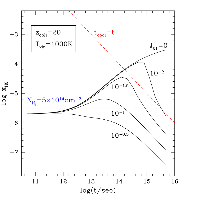
Figure 5.— Evolution of the ${\rm H_{2}}$ abundance in the core of the singular isothermal sphere shown in Figure 4; in the presence of various UV background fluxes (solid lines). Also shown is the ${\rm H_{2}}$ abundance at which the cooling time equals the time elapsed since the collapse of the cloud (short dashed line); and the ${\rm H_{2}}$ abundance at which the LW lines would become self–shielding (at an integrated ${\rm H_{2}}$ column density of $5\times 10^{14}~{}{\rm cm^{-2}}$, long dashed line). For $J>10^{-1.5}$ the cloud becomes self–shielding, but still cannot cool fast enough.

The evolution of $x_{\rm H_{2}}$ at the core radius $r=r_{0}$ is also shown by the middle solid curves in Figure 5 for various $J_{21}$. The shell at $r=r_{0}$ is normally representative of the whole core, because the density, as well as $x_{\rm H_{2}}$, is flat within $r<r_{0}$ (in some cases, however, the ${\rm H_{2}}$ fraction may still rise within the core, see § 6 below). For comparison, in this Figure we also show the evolution of $x_{\rm H_{2}}$ in the same shell under less intense ($J_{21}=0$ or $10^{-2}$) or stronger ($J_{21}=10^{-1}$ or $10^{-0.5}$) UV backgrounds. In the absence of any UVB, the ${\rm H_{2}}$ fraction rises continuously, and reaches $10^{-3}$ in a Hubble time (top curve); when a flux is turned on and increased (bottom 4 solid curves), the ${\rm H_{2}}$ fraction is continuously suppressed.

By performing similar calculations for clouds with virial temperatures and collapse redshifts in the ranges $10^{2}<T_{\rm vir}<10^{4}$K and $5<z_{\rm coll}<50$, we have found that the evolution shown in Figures 4 and 5 remains qualitatively the same in all cases. However, the level of flux required at which the ${\rm H_{2}}$ molecules are photo–dissociation depends on the values of both $z_{\rm coll}$ and $T_{\rm vir}$.

3.2. The ${\rm\bf H_{2}}$ Abundance and Criterion for Star Formation

In order for a cloud to fragment into stars, or continue collapsing to form a central black hole, it is necessary for the gas to radiate efficiently. A rough estimate of the “critical” ${\rm H_{2}}$ fraction can be obtained by requiring that the cooling time is shorter than either the dynamical time (HRL97), or the Hubble time (Tegmark et al 1997). Here we adopt a somewhat more elaborate criterion for star formation, as follows. For a given combination of $z_{\rm coll}$, $T_{\rm vir}$, and $J_{21}$, the cloud is assumed to be able to cool if, at any time during its evolution, the cooling time in the core exceeds the “present time”, defined as the time elapsed since the formation of the cloud at $z_{\rm coll}$. We assume this to be both a necessary and a sufficient criterion.

This definition explicitly takes into account the behaviour of the ${\rm H_{2}}$ fraction shown in Figures 4 and 5, especially the fact that the ${\rm H_{2}}$ fraction in the core first rises and then declines again. Our criterion imposes the requirement that the cloud not spend more than a cooling time at a given ${\rm H_{2}}$ fraction, before the ${\rm H_{2}}$ abundance is further reduced by photo–dissociation. This definition avoids star formation in a situation when the cooling time exceeds the dynamical time, but only for a brief interval that would be too short for a significant contraction to take place. In Figure 5, our criterion is implemented by requiring that the solid line (the evolving ${\rm H_{2}}$ fraction) goes above the short–dashed line (the critical ${\rm H_{2}}$ fraction at which $t_{\rm cool}$ equals the present time $t$).

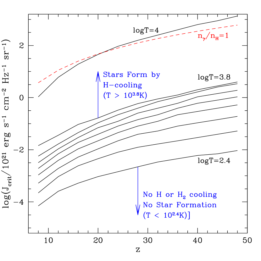
Figure 6.— The critical flux above which star formation in a halo with virial temperature $T_{\rm vir}$ and collapse redshift $z_{\rm coll}$ is prevented. Halos smaller than $T_{\rm vir}\approx 10^{2.4}$K cannot cool even in the absence of any flux. Halos larger than $T_{\rm vir}\approx 10^{3.8}$K can cool via atomic H, irrespective of the ${\rm H_{2}}$ abundance. For comparison, the dashed curve show the flux corresponding to one ionizing photon per H atom, the minimum flux necessary to reionize the universe.

Interestingly, we find that the cloud may undergo a brief interval during which it is self–shielding in the ${\rm H_{2}}$ LW bands, but then may become optically thin again as the ${\rm H_{2}}$ abundance drops due to subsequent photo–dissociation. This is demonstrated in Figure 5: the long dashed line shows the value of $x_{\rm H_{2}}$ that would imply an integrated ${\rm H_{2}}$ column density of $N_{\rm H_{2}}=5\times 10^{14}~{}{\rm cm^{-2}}$ across the cloud, at which the LW lines become self–shielding. As the figure shows, if the flux is below $J_{21}\approx 10^{-0.7}$, the ${\rm H_{2}}$ fraction does temporarily rise above this critical value; but for $J_{21}\;\hbox to0.0pt{\lower 2.5pt\hbox{$\sim$}\hss}\raise 1.5pt\hbox{$>$}\;10^{-1.5}$, our criterion for star formation is still not satisfied. This implies that self–shielding by itself does not guarantee that the molecules are preserved and enable efficient cooling. Requiring the cloud simply to self–shield would therefore not be a good star formation criterion. However, the decline in the H₂ fraction is due to the decreasing electron abundance which lowers the H₂ formation rate. Hence, if an additional process keeps the $e^{-}$ fraction greater than $\sim 10^{-5}$, more H₂ could be formed. This possibility is discussed in greater detail in § 6.

3.3. The Minimum Flux for Negative Feedback

In addressing the effect of the feedback from the UVB, the main question is: given a collapsed cloud with $z_{\rm coll}$ and $T_{\rm vir}$, what is the critical value of the background flux, $J_{\rm crit}$ so that star–formation in this collapsed cloud is suppressed? In the example shown in Figures 4 and 5, $(z_{\rm coll},T_{\rm vir})=(20,10^{3}{\rm K})$, $J_{\rm crit}$ can be read off directly from Figure 5, $J_{\rm crit}=10^{-1.5}$. In order to be able to investigate the evolution of the UVB in the Press–Schechter models, we have repeated the same calculation for a grid of values for $5<z_{\rm coll}<50$, and $2<\log(T_{\rm vir}/{\rm K})<4$. For each pair of values, we have found the critical flux for preventing star formation, $J_{\rm crit}$.

The resulting $J_{\rm crit}=J_{\rm crit}(z_{\rm coll},T_{\rm vir})$ are shown in Figure 6. In general, the higher the density (or $z_{\rm coll}$) or temperature, the higher the flux needs to be to prevent star formation. We have also found that for temperatures below $\log(T_{\rm vir}/{\rm K})<2.4$, the value of the flux becomes irrelevant for star formation, because the cooling function of ${\rm H_{2}}$ drops, and ${\rm H_{2}}$ cooling is inefficient at these low temperatures, even in the absence of any flux. Similarly, the value of the flux is irrelevant for $\log(T_{\rm vir}/{\rm K})>3.8$, because at these high temperatures, cooling from (collisional excitations of) neutral H always dominates over ${\rm H_{2}}$ cooling, i.e. stars can form irrespective of the ${\rm H_{2}}$ abundance.

The values of $J_{\rm crit}$ shown in Figure 6 are relatively low. For reference, the dashed curve in this figure shows the value of $J_{\rm crit}$ that corresponds to one ionizing photon per hydrogen atom, i.e. the minimum flux necessary to reionize the universe. Since the values of the flux necessary to prevent star–formation are 2–4 orders of magnitude below this minimum reionizing flux, a negative feedback necessarily turns on prior to reionization. If the star formation efficiency was a universal constant inside all halos that can cool efficiently, independent of redshift and halo size, then the negative feedback would turn on long before reionization – when the collapsed fraction of baryons $f_{\rm coll}$ is $\sim$4 orders of magnitude smaller then it is at reionization – and it would last until $f_{\rm coll}$ rises by a factor of $\sim 100$.

Since new sources appear exponentially fast in the Press–Schechter formalism, the relatively “long” interval in $f_{\rm coll}$ can translate into a “short” interval in redshift. However, it is clear from the above that the fundamental “evolutionary parameter” for the negative feedback, followed by reionization, is $f_{\rm coll}$, rather than the redshift to which it translates to. Our results may therefore vary in different cosmologies when stated in terms of redshift, but would be relatively robust to change in the background cosmology, when stated in terms of $f_{\rm coll}$. Finally, we emphasize that the actual redshift (and $f_{\rm coll}$) interval between the turn–on of the negative feedback and reionization would be shorter if the star–formation efficiency in small halos is intrinsically much smaller than in large halos (see discussion below).

4. ${\rm\bf H_{2}}$–Feedback and the Buildup of the Cosmic UV Background

In this section, we put together the results of the previous sections to compute the redshift evolution of the UV background, the intergalactic ${\rm H_{2}}$ fraction, and the mass–scale of the ${\rm H_{2}}$ feedback. The latter is more conveniently expressed by defining a critical virial temperature, $T_{\rm crit}(z)$, that corresponds to the minimum size of a cloud that satisfies our star formation criterion under a fixed UV background $J_{21}$ and collapse redshift $z_{\rm coll}$. The evolution of $T_{\rm crit}(z)$ and the UVB amplitude, $J_{21}(z)$ are then coupled together, since $T_{\rm crit}(z)$ is directly determined by $J_{21}(z)$, and conversely, $J_{21}(z)$ depends on the $T_{\rm crit}(z)$ above which we allow halos to contribute to the UVB. As argued above, the evolution of the intergalactic ${\rm H_{2}}$ can be considered separately, since it does not modulate the UVB at the level that would alter the ${\rm H_{2}}$ photodissociation rate inside halos.

Our model is based on the Press–Schechter formalism. We assume that the mass–function of dark halos is given by the Press–Schechter formula, $N_{\rm ps}(z,M)$. The mass function of collapsed baryonic clouds is obtained from $N_{\rm ps}(z,M)$ by the simple replacement $M\rightarrow\Omega_{\rm b}/\Omega_{\rm tot}M$. For the smallest masses, near the Jeans mass ($M\sim 10^{4-5}{\rm M_{\odot}}$), we apply a correction to take into account the non–zero gas pressure in these clouds. This is achieved by replacing $M\rightarrow f_{\rm b}\Omega_{\rm b}/\Omega_{\rm tot}M$, where $0\leq f_{\rm b}\leq 1$ is the fraction of baryons that settle in the potential well of a dark halo of mass $M$ by redshift $z$ (Haiman & Loeb 1997). We use the mass–virial temperature relation of the TIS solutions. Although this relation was derived in a standard CDM cosmology, the scaling of $T_{\rm vir}$ with redshift is changed only negligibly in our $\Lambda$CDM cosmology at the high redshifts of interest.

To parameterize the uncertainties regarding the ionizing photon production rate per collapsed baryon, we assume that each halo (provided it satisfies the star formation criterion) has a constant star formation rate for $t_{\rm on}$ years, during which it turns a total fraction $\epsilon$ of its baryonic mass into stars with a Scalo IMF. This parameterization could correspond to different physical scenarios. For instance, $\epsilon$ would remain the same if the star formation rate in each halo was doubled, but the escape fraction of ionizing photons reduced to 50%. Similarly, a nominal $\epsilon>100\%$ could correspond to a ”top heavy” IMF biased towards massive stars relative to Scalo, so that the number of UV photons produced per collapsed baryons is increased. We do not attempt to summarize all the relevant uncertainties here (instead, see Haiman & Loeb 1997), and view $t_{\rm on}$ and $\epsilon$ as representative parameters in the simplest possible model. It is important to note, however, that a combination of these parameters is constrained by the reionization redshift $6\;\hbox to0.0pt{\lower 2.5pt\hbox{$\sim$}\hss}\raise 1.5pt\hbox{$<$}\;z\;\hbox to0.0pt{\lower 2.5pt\hbox{$\sim$}\hss}\raise 1.5pt\hbox{$<$}\;40$ (Haiman & Knox 1999), requiring that a few ionizing photons per hydrogen atom be produced within this redshift interval.

Within this model, we start from a high redshift ($z=200$), and take small redshift steps towards z=0. At each step, the background flux is obtained by summing the flux of all sources that are within the imaginary redshift screen at $z_{\rm max}$ as discussed in § 2.1, and satisfy the star formation criterion of § 3.2,

$$J_{21}(z,\nu)=\int_{z}^{z_{\rm max}}dz^{\prime}c\frac{dt}{dz^{\prime}}j_{\nu^{\prime}}(z^{\prime}),$$ (7)

where $j_{\nu}(z)$ is the total emissivity from all luminous halos at redshift $z$ and frequency $\nu$,

$$j_{\nu}(z)=\frac{3.7\epsilon}{t_{\rm on}}\int_{z}^{z+dz(t_{\rm on})}dz^{\prime}\frac{dF(z^{\prime},T_{\rm crit}[z^{\prime}])}{dz^{\prime}},$$ (8)

where $F(z,T_{\rm crit}[z])$ is the total fraction of baryons in collapsed halos with virial temperatures above $T_{\rm crit}$. Here $t_{\rm on}$ is in units of seconds, and $j_{\nu}(z)$ is in $10^{-21}~{}~{}{\rm erg~{}s^{-1}~{}cm^{-3}~{}Hz^{-1}~{}sr^{-1}}$.

Once this flux is obtained, we find the critical virial temperature numerically for the new flux $J_{21}$ and redshift, using the information contained in Figure 6.

5. Results

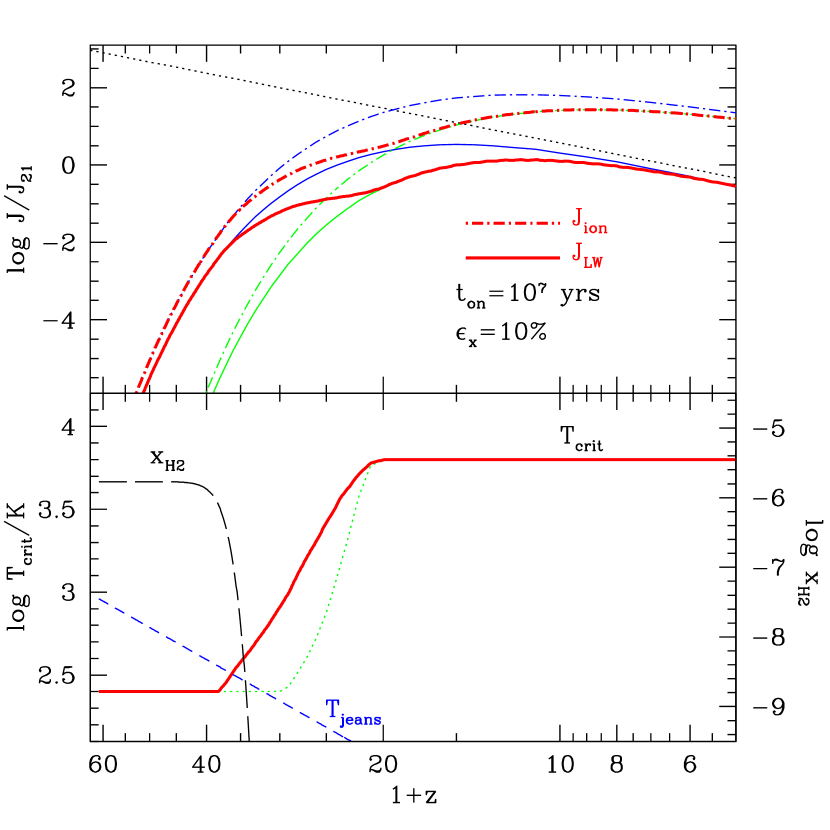
Figure 7.— Coupled evolution of the background flux $J$, critical virial temperature $T_{\rm crit}$, and intergalactic ${\rm H_{2}}$ fraction $x_{\rm H_{2}}$. We assume a UV production efficiency $\epsilon$=10% and source life time $t_{\rm on}=10^{7}$yrs. Upper panel: The evolution of the ionizing flux at 13.6eV (dot–dashed lines) and the average flux in the LW bands (solid lines). In both cases, the bottom and top curve assume a constant $T_{\rm crit}=10^{3.8}K$, and $10^{2.4}K$, respectively, and bracket our actual coupled solution, shown by the thick middle curve. The diagonal dotted line shows the minimum flux for reionization, corresponding to one photon per hydrogen atom. Lower panel: The evolution of the critical virial temperature in the coupled solution (thick solid curve), and using only the flux from halos with $T_{\rm vir}>10^{3.8}$K (dotted curve). The long–dashed line shows the evolution of the ${\rm H_{2}}$ fraction in the IGM. The short–dashed line shows the virial temperature of the mass scale that is just Jeans unstable at each redshift.

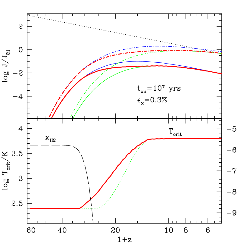
Figure 8.— Same as Figure 7, but assuming $\epsilon$=0.3%.

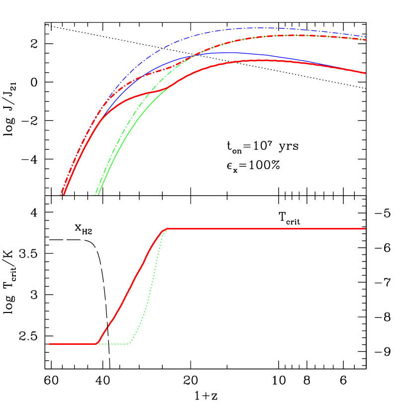
Figure 9.— Same as Figure 7, but assuming $\epsilon$=100%.

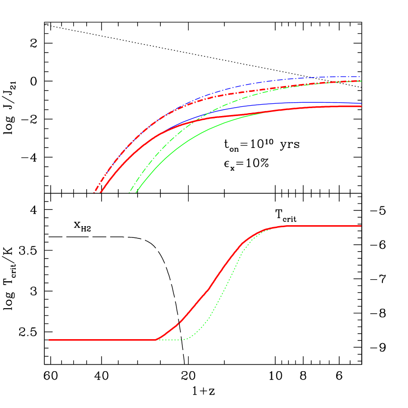
Figure 10.— Same as Figure 7, but assuming $t_{\rm on}=10^{10}$ yrs.

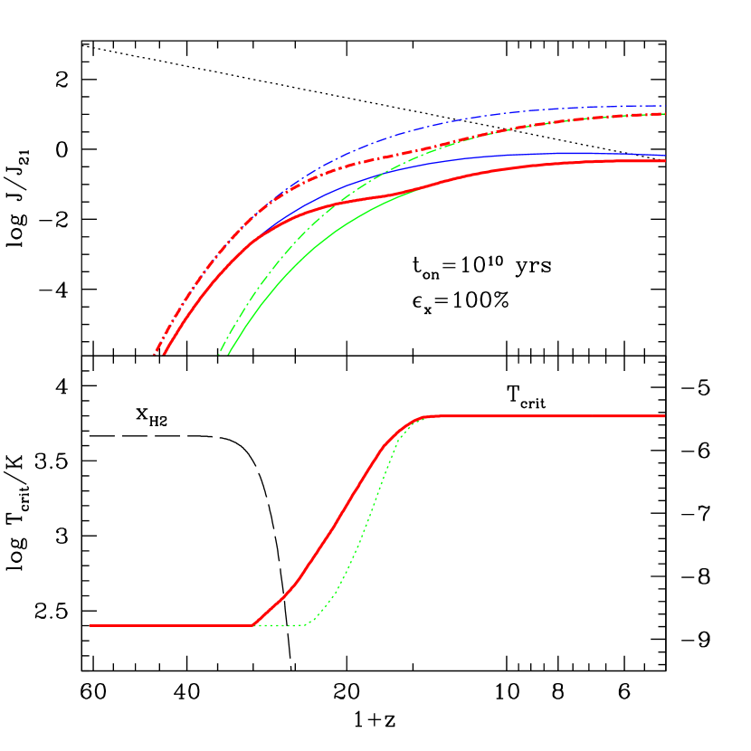
Figure 11.— Same as Figure 10, but assuming $\epsilon$=100%.

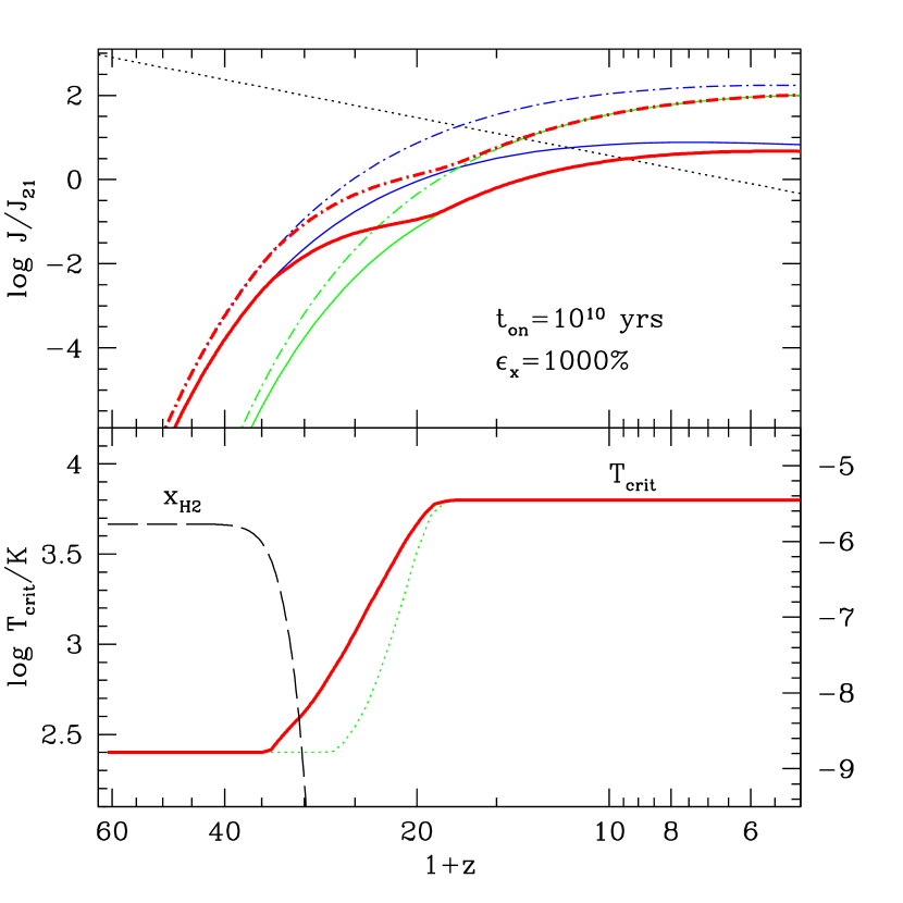
Figure 12.— Same as Figure 10, but assuming $\epsilon$=1000%.

Our main results are shown for six different combinations of lifetime and star formation efficiency ($t_{\rm on}$,$\epsilon$) in Figures 7– 12. In each case, the figure shows the evolution of the ionizing flux at 13.6 eV ($J_{\rm ion}$); the average flux in the LW bands, ($J_{rmLW}$); the critical virial temperature $T_{\rm crit}$; and the intergalactic ${\rm H_{2}}$ fraction.

Figure 7 shows the results in a model with ($t_{\rm on}$,$\epsilon$) = ($10^{7}~{}{\rm yr},10\%$). The three solid curves in the top panel show the evolution of $J_{\rm LW}$ in our model with feedback (middle curve), assuming that the critical virial temperature is fixed at $T_{\rm vir}=10^{2.4}$K (upper curve), and at $T_{\rm vir}=10^{3.8}$K (lower curve). The solid line in the bottom panel shows the evolution of the actual critical temperature, $T_{\rm crit}$, in the coupled solution. These curves demonstrate that initially the small halos are allowed to form stars, there is no feedback, and the flux builds up as in the constant $T_{\rm vir}=10^{2.4}$K case. At redshift $z\approx 35$, the feedback starts to be noticeable, as the flux builds up to $J_{\rm LW}\approx 10^{-2}$, and $T_{\rm crit}$ rises above $10^{2.4}$K. By redshift $z=20$, $T_{\rm crit}$ reaches $10^{3.8}$K. The dot–dashed lines in the top panel show the corresponding evolution of the ionizing flux, $J_{\rm ion}$; and the dotted line shows the minimum flux required for reionization (corresponding to one photon per hydrogen atom). As the figure shows, reionization in this model occurs at $z\sim 15$, and at this redshift the contribution from the small halos to $J_{\rm ion}$ is only $\sim$10% percent. The long dashed line in the bottom panel shows the evolution of the intergalactic ${\rm H_{2}}$ fraction. As expected, $x_{\rm H_{2}}$ drops rapidly to a negligible value by $z=35$, i.e. before the ${\rm H_{2}}$–feedback turns on. This justifies our neglect of the modulation of the UVB by the intergalactic ${\rm H_{2}}$. The short–dashed line shows the virial temperature of the mass scale that is just Jeans unstable at each redshift. This shows that the initial IGM pressure plays a role only for the smallest halos at the highest redshifts.

The next two figures illustrate the effect of changing the total star formation efficiency (or alternatively, the efficiency of UV photon production per collapsed baryon). Figure 8 is analogous to Figure 7, but $\epsilon$ is lowered to $0.3\%$, the smallest possible value that still produces reionization by $z=5$. The evolution is qualitatively similar to the $\epsilon=10\%$ case: the ${\rm H_{2}}$ feedback is active during the redshift interval $13\;\hbox to0.0pt{\lower 2.5pt\hbox{$\sim$}\hss}\raise 1.5pt\hbox{$<$}\;z\;\hbox to0.0pt{\lower 2.5pt\hbox{$\sim$}\hss}\raise 1.5pt\hbox{$<$}\;30$, before reionization takes place at $z\approx 5$. The star formation in small halos is suppressed, and their contribution to the background flux at $z=5$ is only $\sim 4\%$, less than in the $\epsilon=10\%$ case. This, however, is mostly an intrinsic effect, rather than a result of the negative feedback: as shown by the convergence of the top and bottom dashed curves, by the late time when reionization occurs, the background ionizing flux is anyway dominated by the large halos. The figure also shows that the negative feedback has a smaller effect than in the $\epsilon=10\%$ case (the middle and top dashed lines differ by a smaller factor). This is because the background flux builds up more slowly, and the feedback is delayed to a later redshift. By this later redshift, a larger fraction of the small halos have collapsed and formed stars.

Figure 9 demonstrates the opposite effect of increasing the star formation efficiency to a nominal $\epsilon=100\%$. In this case, reionization occurs earlier, at $z\approx 19$, and the ${\rm H_{2}}$ feedback operates at the earlier epoch between $24\;\hbox to0.0pt{\lower 2.5pt\hbox{$\sim$}\hss}\raise 1.5pt\hbox{$<$}\;z\;\hbox to0.0pt{\lower 2.5pt\hbox{$\sim$}\hss}\raise 1.5pt\hbox{$<$}\;42$. As shown by the large difference between the top and middle dashed curves, the negative feedback is more pronounced, and it suppresses star formation in a larger fraction of the small halos. The total contribution of small halos to the ionizing flux at $z=19$ in this case is $\sim 9\%$. In the absence of the feedback, the small halos would dominate the flux by a factor of more than 10 at $z=19$, and reionization would occur at $z\sim 25$.

Figures 10– 12 demonstrate the effect of increasing the source lifetime, $t_{\rm on}$ to $10^{10}$ yrs. This long lifetime would also mimic the scenario in which constant mergers result in multiple recycling of the gas (originally associated with a given halo) for star formation. Making the nominal lifetime longer is equivalent to decreasing the star formation rate, and has an effect similar to decreasing $\epsilon$: the buildup of the background flux is now delayed (although not eventually suppressed as it is when $\epsilon$ is decreased). As a result, the reionization redshift is delayed. When $\epsilon$=10%, then reionization is at $z\approx 5$, and the ${\rm H_{2}}$ feedback takes place in the interval $10\;\hbox to0.0pt{\lower 2.5pt\hbox{$\sim$}\hss}\raise 1.5pt\hbox{$<$}\;z\;\hbox to0.0pt{\lower 2.5pt\hbox{$\sim$}\hss}\raise 1.5pt\hbox{$<$}\;25$. The total contribution to the reionizing flux from small halos is nevertheless still negligible, only about 2%. Figures 11 and 12 show what happens when $\epsilon$ is increased to 100 or 1000% (note that it can not be decreased below 10% because then reionization would occur at $z<5$). In both cases, the ${\rm H_{2}}$ feedback turns on before reionization, and small halos contribute a negligible amount to the reionizing flux ($5\%$ at $z=10$ and $7\%$ at $z=14$, respectively).

In summary, Figures 7– 12 demonstrate that in all cases, the ${\rm H_{2}}$ feedback suppresses star formation inside the small halos, and that the contribution of the small halos to the reionizing flux is always below 10%. If reionization occurs late, then the ${\rm H_{2}}$ feedback makes little difference to the overall ionizing flux: the contribution from small halos to the reionizing flux is then small in any case, since by this late time, the collapsed baryon fraction, as well as the UV background, is dominated by the large halos even in the absence of the ${\rm H_{2}}$ feedback. This is the case in Figures 8 and 10. This would be especially true in different cosmologies, where structure forms earlier, so that by the time of a late reionization, the dominance of larger halos is even more pronounced. Although not important for reionization in these late–reionization models, the ${\rm H_{2}}$ feedback is still expected to occur. On the other hand, in models which would predict earlier reionization, primarily due to the small halos, the negative ${\rm H_{2}}$ feedback is more pronounced. In these models, it is the feedback that limits the contribution of the small halos to reionization, and delays reionization until larger halos form.

Although we have assumed a universal star formation efficiency, stars in small and large halos are likely to form differently, since the cooling mechanisms are different in the two cases. Thus, there is no a–priori reason to expect the same star formation efficiency in these two different environments. There is a preliminary indication from 3–D simulations that the efficiency in small halos might indeed be small ($<1\%$, Abel et al). If the star formation efficiency in the small halos were intrinsically much smaller than in the large halos, then the contribution to the flux from the small halos would be small, regardless of the ${\rm H_{2}}$–feedback. We emphasize that the ${\rm H_{2}}$ feedback described here would still occur prior to reionization, since the flux from the rare large halos alone is sufficient to suppress star formation inside the small halos. Note that this scenario is different from the one presented in, e.g. Figure 7, since in that case the small halos exert a feedback on their own population, while here the “feedback” is from a distinct population of larger halos. This is demonstrated explicitly in Figures 7– 12, where the dotted curves in each bottom panel shows the critical virial temperature $T_{\rm crit}$, obtained from the UV background due only to the large halos. As these figures show, in all cases, $T_{\rm crit}$ still rises above $10^{2.4}$K and reaches $10^{3.8}$K before reionization.

It is not surprising that the ${\rm H_{2}}$ feedback generically occurs in any model that satisfies the reionization constraint by $z=5$. This is because, as we have shown in § 3.3, the suppression of the ${\rm H_{2}}$ abundance and star formation inside clouds with the relevant range of densities and temperatures requires a UV flux that is only a fraction $10^{-2}-10^{-4}$ of the minimum flux level required for reionization (one photon per hydrogen atom). As the UVB builds up to the reionizing level, it must necessarily first reach the level at which the ${\rm H_{2}}$ feedback sets in.

6. Early Mini–Quasars and the Effects of X–rays

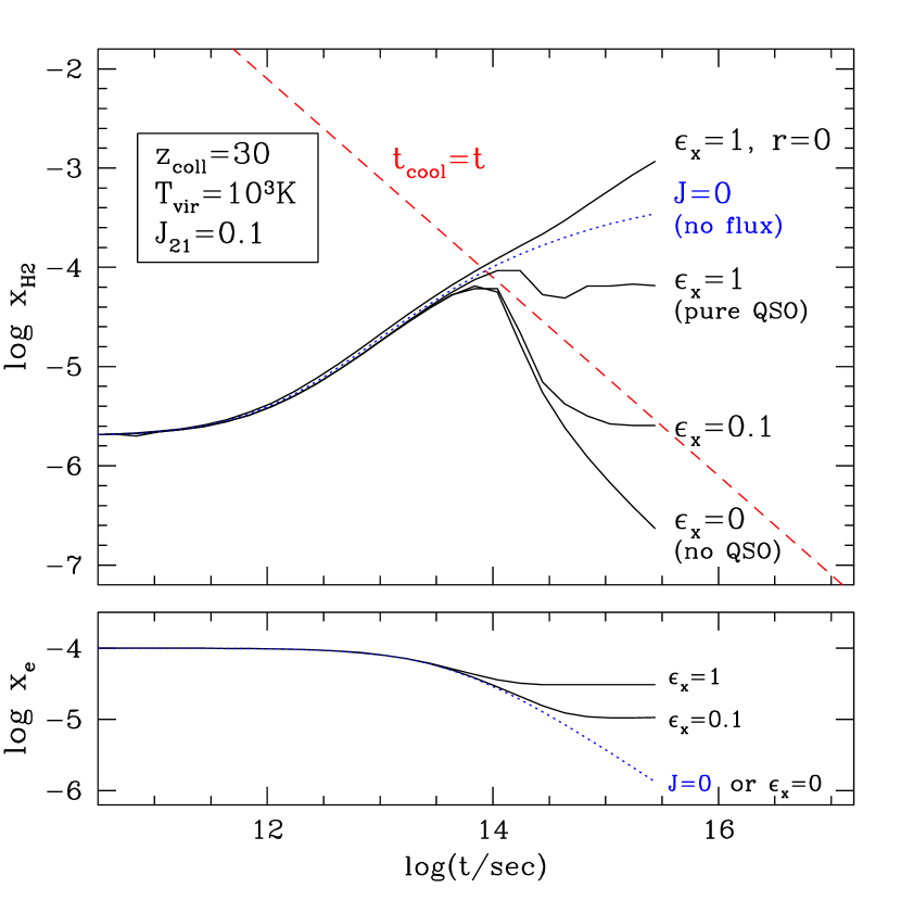
Figure 13.— Effect of X–rays on the evolution of the ${\rm H_{2}}$ abundance. The top panel is similar to Figure 5, except that $z_{\rm coll}=30$, and $J_{21}=0.1$, and we have added an X–ray contribution to the background flux. The curve labeled J=0 shows the evolution of the ${\rm H_{2}}$ abundance in the absence of any flux. The label $\epsilon_{\rm x}$ on the other curves is a measure of the X–ray/UV flux ratio, where $\epsilon_{\rm x}=0$ corresponds to a pure stellar spectrum with no X–rays, and $\epsilon_{\rm x}=1$ corresponds to a pure “mini–quasar” spectrum with a spectral index of -1. The bottom panel shows the evolution of the free electron fraction in each case.

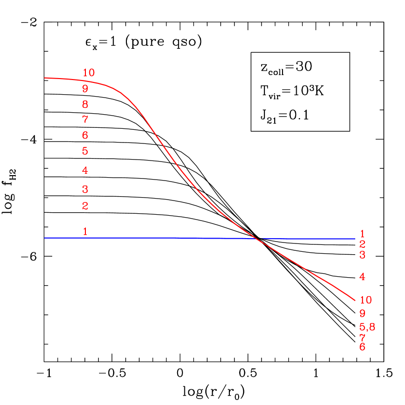
Figure 14.— Effect of X–rays on the profile of the ${\rm H_{2}}$ abundance, for the same truncated isothermal sphere as in Figure 13. Increasing numbers correspond to equal time–steps in logarithmic time, upto a Hubble time of $\sim 3\times 10^{15}$ sec. Note that the ${\rm H_{2}}$ fraction still rises within the core $r<r_{0}$ by an order of magnitude.

So far, we have assumed that the early sources have “stellar” spectra, and have simply truncated the observed flux above 13.6 eV. Since all of our results above depend on the flux only in a narrow frequency range below 13.6eV, they are indeed insensitive to the precise shape of the spectrum.

An alternative possibility is that a halo collapsing at high redshift forms a central black hole, and turns into a ”mini–quasar”, with a hard spectrum extending into the X-ray regime (Haiman & Loeb 1998). The ionization cross–section of neutral hydrogen drops rapidly with frequency (as $\nu^{-3}$), and at frequencies above $h\nu\;\hbox to0.0pt{\lower 2.5pt\hbox{$\sim$}\hss}\raise 1.5pt\hbox{$>$}\;1$keV, the neutral IGM is optically thin. If the spectra of the early sources have a non–negligible contribution at these frequencies, they would establish an early X–ray background (XRB), and change the chemistry qualitatively.

The importance of the X–rays is that they provide additional free electrons, both by direct photo–ionization of H and He, as well as indirectly, by collisional ionization of H by the fast photo–electrons. The resulting extra free electrons catalyze the formation of $H^{-}$, and therefore tend to increase the ${\rm H_{2}}$ abundance. In an earlier paper (HRL96), we have found that inside dense regions ($n_{\rm H}\;\hbox to0.0pt{\lower 2.5pt\hbox{$\sim$}\hss}\raise 1.5pt\hbox{$>$}\;1~{}{\rm cm^{-3}}$), the overall effect of a background flux extending to hard X–rays is to enhance, rather than to suppress, the ${\rm H_{2}}$ abundance. The central densities of centrally condensed virialized clouds are expected to reach $n_{\rm H}\sim 1~{}{\rm cm^{-3}}$. In the case of the TIS solutions adopted here, this density is exceeded for halos that collapse at $z_{\rm coll}\;\hbox to0.0pt{\lower 2.5pt\hbox{$\sim$}\hss}\raise 1.5pt\hbox{$>$}\;7$, and therefore a positive feedback is expected when the UV and X–ray backgrounds together illuminate these halos.

In order to illustrate the effect of the X–rays, we have recomputed the evolution of the ${\rm H_{2}}$ profiles in the TIS models. These computations are identical to the ones discusses in § 3.1, except that the flux in equation 6 is modified to

$$\small{J_{\nu}=\left\{\matrix{J_{21}\left(\frac{\nu}{\nu_{\rm H}}\right)^{-1}\times{\rm sawtooth},\hfill&h\nu<13.6{\rm eV}\hfill\cr\epsilon_{\rm x}J_{21}\left(\frac{\nu}{\nu_{\rm H}}\right)^{-1}e^{(-10^{22}[\sigma_{\rm H,\nu}+0.08\sigma_{\rm He,\nu}])},\hfill&13.6-10{\rm keV}\hfill\cr 0,\hfill&h\nu>10{\rm keV}\hfill\cr}\right.}$$ (9)

Here $\sigma_{\rm H,\nu}$ and $\sigma_{\rm He,\nu}$ are the ionization cross–sections of H and He, and the exponential factor mimics the absorption above 13.6 eV by the neutral IGM by assuming a fixed hydrogen column density of $N_{\rm H}=10^{22}~{}{\rm cm^{-2}}$ and a helium column density a factor of 0.08 smaller. The fiducial value for $N_{\rm H}$ was chosen based on a comparison of background fluxes computed in our Press–Schechter model with and without absorption by neutral H and He at $z=20$. The units of $J_{21}$ are $10^{-21}~{}~{}{\rm erg~{}s^{-1}~{}cm^{-2}~{}Hz^{-1}~{}sr^{-1}}$. We have also introduced a parameter $\epsilon_{\rm x}$ to characterize the ratio of X–ray to UV flux: for pure stellar sources, $\epsilon_{\rm x}=0$; for typical quasar spectra (Elvis et al.), $\epsilon_{\rm x}\sim 1$. Values of $\epsilon_{\rm x}$ in–between 0 and 1 could describe either miniquasars with softer spectra, or a mixed population of stars and mini–quasars. We have verified that our conclusions are not sensitive to the upper energy cutoff, provided this cutoff is above $\sim$1keV.

In Figure 13, analogously to Figure 5, we show the evolution of the ${\rm H_{2}}$ fraction at the core radius of a TIS. For this illustrative example, we assumed that the TIS has $z_{\rm coll}=30$ and $T_{\rm vir}=10^{3}$K, and that it is illuminated by a flux with $J_{21}=0.1$ and $\epsilon_{\rm x}=0,0.1,$ and 1, corresponding to increasing amounts of X–ray contribution. As in the example shown in Figure 5, in the absence of any flux the ${\rm H_{2}}$ fraction rises continuously, in this case to $\sim 10^{-3.5}$ (dotted curve). If the UVB is turned on, the final ${\rm H_{2}}$ fraction is suppressed to $\sim 10^{-7}$ (bottom solid curve). However, if increasing amounts of X–rays are also added (solid curves, second and third from the bottom), then the ${\rm H_{2}}$–suppression (relative to the dotted curve) is less pronounced.

We find that a $\sim$ 10% X-ray contribution ($\epsilon_{\rm x}\approx 0.1$) is enough to keep the ${\rm H_{2}}$ fraction at a high enough level ($\sim 10^{-5.5}$) that satisfies our star formation criterion. This is seen in Figure 13, as the solid curve labeled $\epsilon_{\rm x}=0.1$ reaches the short–dashed curve. For still larger X–ray contributions, the final ${\rm H_{2}}$ fraction is even higher. It is interesting to note that deeper inside the cloud, the sign of the feedback is entirely reversed, and the ${\rm H_{2}}$ abundance is increased relative to the case with no flux. The top solid curve in Figure 13 shows the ${\rm H_{2}}$ fraction at the center $r=0$, rather than at the core radius, in the $\epsilon_{\rm x}=1$ case. Indeed, $x_{\rm H_{2}}$ rises above $10^{-3}$, and reaches a $\sim 3$ value than it would in the absence of any background flux. Figure 14 shows the profile of $x_{\rm H_{2}}$ across the cloud at various time–steps, and demonstrates that the ${\rm H_{2}}$ fraction still rises within the core ($r<r_{0}$) by over an order of magnitude. As described above, the enhancement of the final ${\rm H_{2}}$ fraction is due to the additional free electrons produced by the X–rays. The bottom panel in Figure 13 shows the evolution of the electron fraction in each case: as expected, $x_{\rm e}$ is increased by the presence of X–rays.

By experimenting with different combinations of $z_{\rm coll}$ and $T_{\rm vir}$, we have found that the situation shown in Figure 13 is typical of collapsed clouds with $5<z_{\rm coll}<50$ and $10^{2.4}{\rm K}<T_{\rm vir}<10^{4}$K. Generally, a $\sim 10\%$ contribution by X–rays to the flux is sufficient to keep the ${\rm H_{2}}$ fraction high enough to allow star formation, and hence to eliminate the negative feedback caused by the UV background. To arrive at this conclusion, we have imposed our star–formation criterion at the core radius $r=r_{0}$. However, we have also found that at still smaller radii, the ${\rm H_{2}}$ fraction is typically much larger, and can rise above the value expected in the absence of any background flux. Inside the core, net feedback on the ${\rm H_{2}}$ fraction is therefore positive, rather than negative. In summary, we expect that if the early background had a non–negligible contribution from “mini–quasars” with hard spectra, extending to $\sim 1$ keV, then the negative ${\rm H_{2}}$ feedback described here would not occur.

7. Conclusions

We have examined the build–up of the UV background in hierarchical models, based on the Press–Schechter formalism, and its effect on star formation inside small halos that collapse prior to reionization. We have confirmed our previous conjecture that there exists a negative feedback before reionization. Star formation inside small halos shuts off prior to reionization, as an early UV background below builds up below 13.6 eV, and suppresses the ${\rm H_{2}}$ abundance in these halos.

We have also found that as a result, the contribution to the reionizing flux from the small halos is limited to be less than a $\sim$10% percent in any hierarchical model. It is possible that the star formation efficiency via ${\rm H_{2}}$ cooling in small halos is intrinsically small, as indicated by recent 3–D simulations (Abel et al.). The efficiency can also be kept low by internal feedback mechanisms inside each halo, such as destruction of ${\rm H_{2}}$ molecules by an internal UV source (Silk 1977, Omukai & Nishi 1999), or blow–out of the gas by supernovae (Mac Low & Ferrara 1998). In this case, the contribution of the small halos to reionization can be negligible regardless of the existence of the negative feedback. However, we have shown that the negative feedback would still occur from the flux of the large halos alone.

Another possibility is that even though the integrated star formation efficiency is high, the star formation rate is low, so that the UV flux is built up with a significant delay relative to the collapse of the halos. In this scenario, reionization occurs late (near $z\sim 5$), when the collapsed baryon fraction is already dominated by large halos. Again, in this case, the negative feedback would still occur early on, but would not have a significant effect on reionization.

More generally, we have shown that the contribution of the small halos to the reionizing flux is small in essentially any model where the first collapsed halos do not produce hard (E $\sim$$>$ 1keV) X–rays. The reason for this is that the flux necessary to suppress the ${\rm H_{2}}$ abundance and cooling in small halos is $10^{2-4}$ times lower than the minimum flux necessary for reionization, corresponding to an one UV photon per baryon.

Finally, we have shown that the negative feedback would be turned into a positive one if there was a significant ( $\sim$$>$ 10%) contribution to the early UV background from “mini–quasars” with hard spectra extending to the X–rays (upto $\sim$1keV). In this case, the X–rays catalyze the formation of ${\rm H_{2}}$ molecules by providing additional electrons, and the overall effect is to enhance, rather then to suppress, the ${\rm H_{2}}$ abundance. The evolution of the small early halos is therefore distinctly different in stellar and mini–quasar models: this may help shed light on the question of what type of sources were responsible for ending the “dark age”, and reionized the Universe.

Appendix A The Relevant Lyman–Werner Lines of ${\rm\bf H_{2}}$ Molecules

The bulk of the intergalactic H₂ is in the lowest states vibrational and rotational state of the ground electronic state. Hence only v=0 with J=0 (para) and 1 (ortho) are populated. There are numerous Lyman Werner band transitions that can yield photo-dissociation via a decay from excited electronic states to the continuum of two distinct H atoms. These are typically classified as R or P transitions, depending on whether the rotational quantum number changes by -1 or +1 from the electronic ground to the electronic excited state (angular momentum must change due to parity conservation). Hence, assuming that both para and ortho hydrogen molecules are abundant in their ground states, all R(0) [i.e. $J=0\rightarrow J=1$], R(1) [i.e. $J=1\rightarrow J=2$], and P(1) [i.e. $J=1\rightarrow J=0$] transitions are possible, for each excited vibrational level. The above is true both for the Lyman and Werner bands. For the Werner band ($X\,^{1}\Sigma_{g}^{+}-C\,^{1}\Pi_{u}$), there is an additional Q–branch in which $\triangle J=0$ is allowed. Figure 15 illustrates all possible transitions from the lowest energy states of ortho and para H₂.

There is a total of 76 possible transitions from the lowest roto-vibrational state of ortho and para molecular hydrogen that are below the Lyman limit of atomic hydrogen (13.6eV). Figure 16 gives an overview of these 76 lines that are relevant for cosmological H₂ photo–dissociation. The quantity $f_{osc}\times f_{diss}$ quantifies the contribution of an individual line to the overall photo–dissociation. The $J$–dependent dissociation fractions in this figure were taken from Abgrall et al.  (1992). From their work one sees that the dissociation fractions of the Werner Q–branch (which couples to the $\Pi^{-}$ state) are extremely small. For the R–branch, however, the $f_{diss}$ are quite significant (especially for $v^{\prime}=3$ of the Werner band). As the figure shows, photons with $h\nu\;\hbox to0.0pt{\lower 2.5pt\hbox{$\sim$}\hss}\raise 1.5pt\hbox{$<$}\;11.9{\rm\,eV}$ do not contribute significantly to the dissociation rate due to their small $f_{osc}$. In addition, the Werner bands with $v^{\prime}\neq 3$ do not contribute much to the dissociation rate.

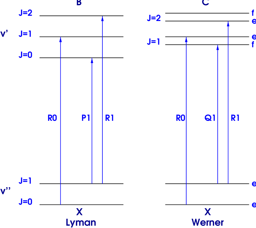
Figure 15.— Illustration of all possible absorption lines from the lowest energy states of ortho and para H₂.

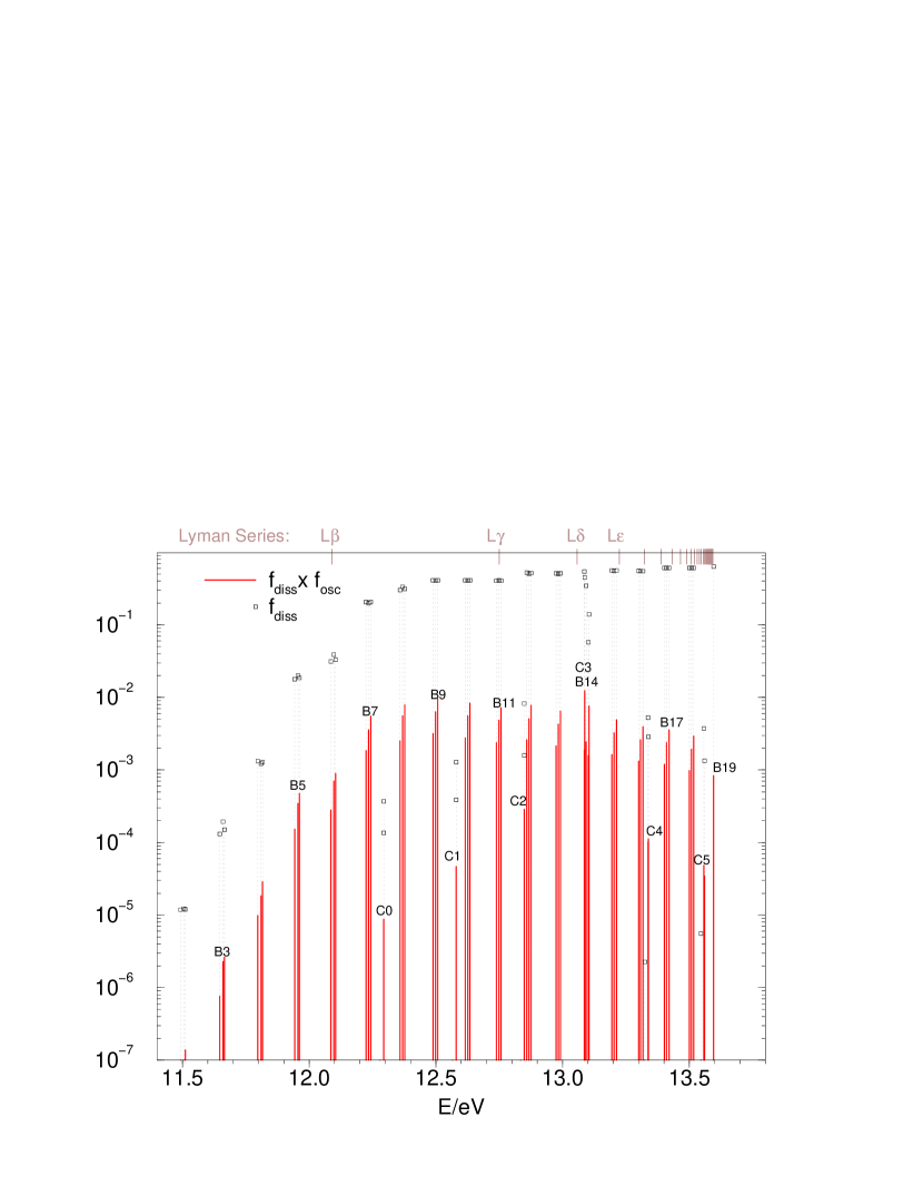
Figure 16.— The relevant Lyman Werner bands for intergalactic H₂ photo-dissociation. The solid columns indicate the value of $f_{diss}\times f_{osc}$ and the dotted ones show the dissociation fractions. Lines of the Lyman (Werner) system are labeled by B$v^{\prime}$ (C$v^{\prime}$) where $v^{\prime}$ is the vibrational quantum number of the excited state. The location of the atomic hydrogen Lyman series are indicated on the top of the graph.

References

- (1)
- (2) Abel, T., & Mo, H. J. 1998, ApJL, 494, 151
- (3)
- (4) Abel, T., Bryan, G. L., & Norman, M. L. 1998, in Proc. of the MPA/ESO Conference ”Evolution of LSS: from Recombination to Garching”, Garching, Germany, Aug. 1998, astro-ph/9810215
- (5)
- (6) Abgrall, H., Bourlot, J. Le, Pineau des Forêts, G., Roueff, E., Flower, D.R., Heck, L. 1992, A&A, 253, 525.
- (7)
- (8) Anninos, P., Zhang, Y., Abel, T., Norman, M. L. 1997, New Ast., 2, 209
- (9)
- (10) Barkana, R., & Loeb, A. 1999, ApJ, submitted, astro-ph/9901114
- (11)
- (12) Elvis, M., Wilkes, B. J., McDowell, J. C., Green, R. F., Bechtold, J., Willner, S. P., Oey, M. S., Polomski, E., & Cutri, R. 1994, ApJS, 95, 1
- (13)
- (14) Field, G. B., Somerville, W. B., and Dressler, K. 1966, ARA&A 4, 207
- (15)
- (16) Haiman, Z., & Knox, L. 1999, in Sloan Summit on Microwave Foregrounds, eds. A. de Oliveira-Costa and M. Tegmark, in press, astro-ph/9902311
- (17)
- (18) Haiman, Z., & Loeb, A. 1997, ApJ, 483, 21
- (19)
- (20) Haiman, Z., & Loeb, A. 1998, ApJ, 503, 505
- (21)
- (22) Haiman, Z., Rees, M. J., & Loeb, A. 1996, ApJ, 467, 522 (HRL96)
- (23)
- (24) Haiman, Z., Rees, M. J., & Loeb, A. 1997, ApJ, 476, 458 (HRL97)
- (25)
- (26) Haiman, Z., Thoul, A., & Loeb, A. 1996, ApJ, 464, 523
- (27)
- (28) Herzberg, G. 1950, Spectra of Diatomic Molecules, Van Nostrand Reinhold Co., New York
- (29)
- (30) Kashlinsky, A., & Rees, M.J. 1983, MNRAS, 205, 955
- (31)
- (32) Kravtsov, A. V., Klypin, A. A., Bullock, J. S., & Primack, J. R. 1998, ApJ, 502, 48
- (33)
- (34) Mac Low, M.-M., & Ferrara, A. 1998, in The Magellanic Clouds and Other Dwarf Galaxies, Proc. of the Bonn/Bochum-Graduiertenkolleg Workshop, held at the Physikzentrum Bad Honnef, Germany, January 19-22, 1998, Eds.: T. Richtler and J.M. Braun, Shaker Verlag, Aachen
- (35)
- (36) Madau, P., Ferguson, H. C., Dickinson, M. E., Giavalisco, M., Steidel, C. C., Fruchter, A. 1996, MNRAS, 283, 1388
- (37)
- (38) Miralda-Escudé, J., Haehnelt, M., & Rees, M. J. 1999, ApJ, submitted, preprint astro-ph/9812306
- (39)
- (40) Navarro, J. F., Frenk, C. S., & White, S. D. M. 1997, ApJ, 490, 493
- (41)
- (42) Omukai, K., & Nishi, R. 1999, ApJL, in press
- (43)
- (44) Press, W. H., & Schechter, P. L. 1974, ApJ, 181, 425
- (45)
- (46) Shapiro, P. R., Iliev, I., & Raga, A. C. 1998, MNRAS, submitted, astro-ph/9810164
- (47)
- (48) Silk, J. 1977, ApJ, 211, 638
- (49)
- (50) Smith, E. P., & Koratkar, A. eds, 1998, Science with the Next Generation Space Telescope, Ast. Soc. of the Pacific Conf. Series, vol. 133
- (51)
- (52) Stecher, T. P., & Williams, D. A. 1967, ApJ, 149, L29
- (53)
- (54) Tegmark, M., Silk, J., Rees, M. J., Abel, T., & Blanchard, A. 1997, ApJ, 474, L1
- (55)