[

Cosmological Limits on the Neutrino Mass from the Ly$\alpha$ Forest

Abstract

The Ly$\alpha$ forest in quasar spectra probes scales where massive neutrinos can strongly suppress the growth of mass fluctuations. Using hydrodynamic simulations with massive neutrinos, we successfully test techniques developed to measure the mass power spectrum from the forest. A recent observational measurement in conjunction with a conservative implementation of other cosmological constraints places upper limits on the neutrino mass: $m_{\nu}<5.5$ eV for all values of $\Omega_{m}$, and $m_{\nu}\lesssim 2.4(\Omega_{m}/0.17-1)$ eV, if $0.2\leq\Omega_{m}\leq 0.5$ as currently observationally favored (both $95\%$ C.L.).

]

Experimental evidence for finite neutrino masses and flavor oscillations continues to mount. Recently the Super-Kamiokande experiment has provided strong evidence that oscillations from $\nu_{\mu}$ to another species involve a mass greater than $\sqrt{\delta m^{2}}=0.07^{+0.02}_{-0.04}$eV [1]. The LSND experiment suggests the existence of $\nu_{\mu}$ to $\nu_{e}$ oscillations with $\sqrt{\delta m^{2}}\sim 0.4$ eV [2]. Finally, the solar neutrino deficit requires $\sqrt{\delta m^{2}}\sim 0.003$ eV [3]. These mass splitting results are consistent with one to three weakly interacting neutrinos in the eV mass range [4].

Neutrinos in this mass range are important cosmologically since, if they exist, they would represent a non-negligible contribution to the dark matter content of the Universe. In units of the critical density, neutrinos contribute $\Omega_{\nu}=Nh^{-2}m_{\nu}/94$ eV, where $h$ is the dimensionless Hubble constant ($H_{0}=100h$ km s^-1 Mpc^-1), and $N$ is the number of degenerate mass neutrinos. As light neutrinos do not cluster on small scales, they retard the gravitational growth of density fluctuations. Any measure of small-scale clustering is thus sensitive to neutrino masses in this range. One such useful measure is the clustering of the intergalactic medium revealed by the absorption features in quasar spectra known as the Ly$\alpha$ forest [5]. As we will discuss below, the Ly$\alpha$ forest has the distinct advantage that clustering properties of the mass distribution can be inferred from it, which greatly facilitates comparisons with theory, and makes large searches of parameter-space possible.

In this Letter, we make use of a recent Ly$\alpha$ forest measurement of the power spectrum of mass fluctuations [6] to place limits on the mass of the neutrino(s). Conversion of the power spectrum measurements into neutrino mass limits requires a framework for cosmological structure formation. There is growing evidence that structure formed by the gravitational instability of cold dark matter (CDM) with adiabatic, Gaussian initial fluctuations. Upcoming Cosmic Microwave Background (CMB) experiments should conclusively determine whether this assumption is a good one [7]. For now, we note that this framework, which we adopt, includes all currently favored models, and also that whatever the true model for structure formation, Ly$\alpha$ forest measurements should respond sensitively to the presence of massive neutrinos.

Our adiabatic CDM dominated universes are described by 6 free parameters: the matter density $\Omega_{m}$, dimensionless Hubble constant $h$, baryon density $\Omega_{b}$, neutrino density $\Omega_{\nu}$, density fluctuation amplitude $A$, and tilt $n$, which define the initial density power spectrum $P_{\rm init}(k)=Ak^{n}$. We also initially assume that spatial geometry is flat, as implied by recent measurements of distant supernovae and CMB anisotropies [8], before investigating the consequences of relaxing this assumption.

We begin by describing the Ly$\alpha$ forest power spectrum measurement method and test it on hydrodynamic simulations. We then apply the observational constraint to the 6 dimensional CDM parameter space to find an upper limit on the neutrino mass. Given this large parameter space, we conservatively employ other cosmological constraints, notably from the abundance of galaxy clusters and the age of globular clusters, to constrain other parameters that can mimic the effects of massive neutrinos. Finally, we consider prospects for making a precise measurement of $m_{\nu}$ using future Ly$\alpha$ forest observations and upcoming CMB experiments.

Testing Ly$\alpha$ forest simulations with $m_{\nu}>0$.— The Ly$\alpha$ forest of neutral hydrogen absorption seen in quasar spectra [5] arises naturally in cosmological scenarios where structure forms by the action of gravitational instability. In hydrodynamic simulations of such models [9] most of the absorption arises in gas of moderate overdensity, whose physical state is governed by simple processes (mainly photoionization heating and adiabiatic cooling, see also the analytical modeling of [10]). The density field can then be locally related to the optical depth for Ly$\alpha$ absorption [11] and hence a directly observable quantity, the transmitted flux in a quasar spectrum.

The Ly$\alpha$ forest can therefore be used to determine the statistical properties of the density distribution, and in particular $P(k)$, the power spectrum of density fluctuations. A method for carrying this out was described by [12], who also tested it on hydrodynamic simulations with CDM only. The method relies explicitly on the assumptions that the initial fluctuations were Gaussian, and that gravitational instability was responsible for their growth. A measurement from an observational dataset was made by [6]. As we will use this result to constrain the neutrino mass, we first test the method on a hydrodynamic simulation which includes massive neutrinos.

The measurement of $P(k)$ from Ly$\alpha$ forest spectra is carried out in two stages. First, the shape of $P(k)$ is measured from the power spectrum of the Ly$\alpha$ forest flux. Second, normalizing simulations are used to set the amplitude of the linear mass $P(k)$. We refer the reader to [12] for details.

The hydrodynamic simulation itself is described in detail by [13]. We follow the evolution of structure in a model with two mass-degenerate neutrino species, using the Parallel TreeSPH hydrodynamic code [14]. The model parameters are $\Omega_{m}=1,h=0.5,\Omega_{b}=0.075$, and $\Omega_{\nu}=0.2$, so that the mass in both species combined is $5$ eV. This so-called cold plus hot dark matter model (CHDM) is normalized to fit the COBE results [15], so that the amplitude of mass fluctuations in $8\ h^{-1}{\rm\,Mpc}$ spheres at $z=0$, $\sigma_{8}=0.7$. We use a box of size $11.111\ h^{-1}{\rm\,Mpc}$, periodic boundary conditions and initial conditions taken from [16]. The CDM and gas components are represented by $64^{3}$ particles each, and the neutrinos by $2\times 64^{3}$ particles. We use the distribution and physical state of the gas at $z=2.5$ to generate artificial Ly$\alpha$ spectra, for 1200 randomly chosen lines of sight through the simulation volume.

We then apply the $P(k)$ recovery method of [12] to these spectra. We use normalizing simulations run under the PM approximation [17, 12] with $64^{3}$ particles and an $11.111h^{-1}{\rm\,Mpc}$ box. We use the same estimator for the amplitude of $P(k)$ as in the observational analysis paper, [6]. The results of the test are shown in Fig. 1, where we plot the recovered $P(k)$, together with the linear theory prediction for the model. We also show the linear power spectrum of a CDM-only model (with $\Omega_{m}=1,h=0.5$), again normalized to COBE, so that $\sigma_{8}=1.2$.

The error bars on the $P(k)$ points are representative of the “cosmic variance” error which arises from only having one hydrodynamic simulation volume. We estimate this uncertainty by running 10 additional PM approximation simulations of the CHDM model, and extracting 1200 lines of sight from each. The standard deviation of their results for each $P(k)$ point provides the error bar. There is an additional overall amplitude uncertainty associated with the normalization. We estimate this by applying the normalizing procedure to the PM CHDM simulations taken individually, finding that the additional error in this test case is a negligible $4\%$ in $P(k)$.

We use the simulation to test for systematic errors in the technique. The observational result was given by [6] in terms of a power law fit to the $P(k)$ data points with $2.7\times 10^{3}{\rm\,(kms^{-1})}^{-1}<k<1.42\times 10^{2}{\rm\,(kms^{-1})}^{-1}$ (which corresponds to $0.5\ h{\rm\,Mpc}^{-1}<k<2.7\ h{\rm\,Mpc}^{-1}$ for an Einstein-de Sitter model). We fit the simulation data points to a power-law over this range, finding an amplitude $\Delta^{2}(k)=0.16\pm 0.028$ ($1\sigma$) at $k=1.5h{\rm\,Mpc}^{-1}$ [$=0.008{\rm\,(kms^{-1})}^{-1}$]. Here $\Delta^{2}(k)=k^{3}P(k)/2\pi^{2}$, the contribution to the density field variance from a unit interval in $\log k$. The logarithmic slope, $n=-2.18^{+0.34}_{-0.28}$ ($1\sigma$). The linear theory prediction for CHDM is $\Delta^{2}(k)=0.21$, $n=-2.40$. Our recovered $P(k)$ is therefore about $2\sigma$ too low in amplitude, and has a slightly flatter slope. By examining results from the more numerous PM simulations, we find that the largest scale data point is systematically lowered by peculiar velocity distortions (as predicted by [18]), an effect which is not accounted for in our estimate of the $P(k)$ shape. Including or leaving out this point (which has the largest statistical errors) has only a small effect on the power law fit. It is possible, however, that taking these effects into account or further refining the analysis would improve the result. For the moment it is sufficient to note that the observational result of [6] currently has a statistical uncertainty of $\sim 70\%$ ($2\sigma$), larger than any biases revealed by our test.

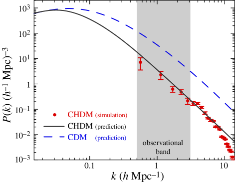
FIG. 1.: A test of the $P(k)$ recovery method. The points are $P(k)$ recovered from a hydrodynamic simulation of the Ly$\alpha$ forest in a massive neutrino model (CHDM see text). The turndown for $k>5h{\rm\,Mpc}^{-1}$ is caused mainly by the limited resolution of the simulation and lies outside of the observational band (shaded). The lines show the linear $P(k)$ predictions for the massive neutrino model, and for a CDM-only model.

Constraining the neutrino mass.— Although the suppression of power in the Ly$\alpha$ forest due to a finite neutrino mass is large ($\sim 800\Omega_{\nu}/\Omega_{m}$ percent [19]), other aspects of the cosmological model can counterbalance this effect; limits on the neutrino mass consequently depend on the range of models allowed by other cosmological constraints.

In addition to the Ly$\alpha$ forest power spectrum measurement of $\Delta^{2}(0.008[$ km s${}^{-1}]^{-1})=0.57^{+0.54}_{-0.27}$ (95% CL) (we do not use the Ly$\alpha$ slope measurement, which has no significant effect) at $z=2.5$, we consider 6 other cosmological constraints. The Hubble constant is measured to be $h=0.72\pm 0.17$ (95% CL), where we have added statistical and systematic errors in quadrature and doubled the $1\sigma$ errors [20]. The amplitude of the fluctuations is determined by the COBE detection of large angle anisotropies [15]; we ignore the 7% measurement uncertainties on the temperature fluctuations which are substantially smaller than the other uncertainties. The abundance of galaxy clusters today constrains models at the 8$h^{-1}$Mpc scale, where the amplitude of fluctuations in top-hat spheres (at $z$=0) is $\sigma_{8}=0.56\Omega_{m}^{0.47}$ with 95% CL of $+20\Omega_{m}^{0.2\log\Omega_{m}}$ percent and $-18\Omega_{m}^{0.2\log\Omega_{m}}$ percent [21].

Galaxy surveys measure the shape of the power spectrum; we use the compilation of [22] and take measurements only from the range $0.025h$ Mpc${}^{-1}<k<0.25h$ Mpc^-1 to avoid spurious survey volume effects on the large scale and uncertainties in the nonlinear corrections on the small scale. For the galaxy survey data, we employ a $\Delta\chi^{2}$ statistic and take $\Delta\chi^{2}=4$ to represent the $95\%$ confidence limits on the shape of the power spectrum. In carrying this out, we assume that a linear “bias” is operating so that the matter power spectrum is related to the galaxy power spectrum by a constant multiplicative factor (which we find as part of our $\chi^{2}$ minimization). We also employ nucleosynthesis constraints on the baryon density of $\Omega_{b}h^{2}=0.019\pm 0.0024$ (95% CL) [23]. Finally, we place a lower limit on the age of the universe by assuming that it must at least as old as the oldest globular clusters $(13.2\pm 2.9)$Gyrs (95% CL) [24]).

Given these constraints, we could construct a joint likelihood to find the best fitting neutrino mass. We have decided to be more conservative, however, and consider a model ruled out if it violates the (95%) confidence limits on any constraint taken individually. With these “$2\sigma$” constraints on the parameter space, we use the analytic approximations of [26] to explore the remaining space rapidly and find the model that maximizes the neutrino mass as a function of $\Omega_{m}$. The result for one massive species is displayed in Fig. 2a. We also show the effect of omitting the Ly$\alpha$ forest measurement. The measurement has a powerful constraining effect at low and high $\Omega_{m}$ since the amount of tilt required to match the cluster abundance and galaxy power spectrum shape violates the upper and lower Ly$\alpha$ forest bounds respectively. For no value of $\Omega_{m}$, can $m_{\nu}$ be greater than $5.5$eV.

To address the robustness of our upper limits, we show the effect of scaling all errors by a factor of 1.5 to approximate “$3\sigma$” constraints in Fig. 2. We also test for single point failures by dropping each constraint sequentially. Omission of either the age or cluster abundance constraint changes the maximal neutrino mass to $\sim 7$eV. While dropping the galaxy power spectrum constraint does not increase the maximal mass substantially, it does weaken the bounds by up to 2 eV for $\Omega_{m}\lesssim 0.5$. Omission of the $h$ or $\Omega_{b}h^{2}$ constraint has essentially no effect.

In applying our constraints, we assume that the universe is flat ($\Omega_{m}+\Omega_{\Lambda}=1$) and that gravity waves do not contribute to the COBE normalization. However, assuming an open universe or gravity waves from power law inflation does not change the $m_{\nu}$ limits significantly since the tilt can be used to offset small changes in normalization. The simplest inflationary models can also predict a variation of the spectral index with scale. This is a small effect compared to the neutrino power suppression, so that we do not include it. Future CMB observations should address this point definitively.

We also show the results assuming 2 neutrino species with identical masses in Fig. 2b. These limits are roughly half the single species results since the change in the growth rate is mainly governed by $\Omega_{\nu}$. However dividing the total mass into 2 species makes each species more relativistic and enhances the suppression of the power on scales relevant to the galaxy power spectrum and cluster abundance constraints [27].

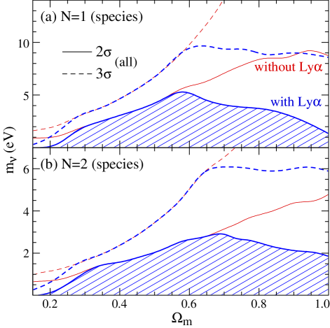
FIG. 2.: Constraints on the neutrino mass (a) single massive species (b) two (degenerate) mass species with and without the Ly$\alpha$ constraint.

Future prospects.— Additional Ly$\alpha$ forest data from quasar surveys such as the Sloan Digital Sky Survey (SDSS [25]) have the potential to increase the precision of these mass constraints substantially. Furthermore, we expect that the next generation of CMB satellites will not only verify the existence of the underlying framework for structure formation, which we currently assume, but also provide limits on the neutrino mass itself.

How precise must these Ly$\alpha$ measurements be to improve on projected CMB limits on the neutrino mass? To answer this question, we employ Fisher information matrix techniques to approximate the joint covariance matrix. For the Ly$\alpha$ forest power spectrum measurement, the Fisher matrix is given by ${\bf F}_{ij}=(\Delta P/P)^{-2}(\partial\ln P/\partial p_{i})(\partial\ln P/\partial p_{j})$. We add this to the CMB Fisher matrix projected for the MAP and Planck satellites including polarization information [28]. The variance of the optimal unbiased estimator of $p_{i}$ marginalized over the other parameters is $(F^{-1})_{ii}$.

A fractional error of $\Delta P/P=0.1$ (1$\sigma$) on the Ly$\alpha$ power spectrum would improve the MAP upper limit from 1.1 eV to 0.54 eV and the Planck limit from 0.51 eV to 0.29 eV both at 2$\sigma$. Note that these represent limits in a wider 10 parameter space including spatial curvature and gravity waves. These improvements would exceed those that can be achieved the SDSS galaxy survey [28]. CMB polarization information here is critical for these improvements since they rely on an absolute normalization of the power spectrum from degree scale anisotropies. Polarization information eliminates the degeneracy between the normalization and the optical depth due to reionization.

Is 10% precision in power achievable from Ly$\alpha$ forest measurements? The constraint in this paper relies on data from $\sim 10$ full quasar spectra [6]. The SDSS quasar survey [25] will yield spectra of roughly similar quality (resolution $2.5$ Å compared to $\sim 1.5$ Å for [6]) for $\sim 10^{5}$ quasars. The mean distance between sightlines in the SDSS will be somewhat larger than the scale on which clustering was measured by [6], so that the decrease in statistical errors will not be too far off the factor $\sim(10^{5}/10)^{1/2}\sim 100$ which would be expected if the sightlines were independent. A $1\sigma$ statistical error of $\Delta P/P<1\%$ should therefore be possible in the future, so that systematic errors will become dominant. Studying larger hydrodynamic simulations should enable us to understand these systematic effects and refine our analysis techniques. The vast size of the SDSS dataset will also enable us to pin down non-gravitational contributions to Ly$\alpha$ forest clustering, for example by analyzing the evolution of the forest with redshift. The signature of massive neutrinos, if they are present, should therefore be obvious, even if $m_{\nu}$ is a fraction of an eV.

RACC acknowledges support from NASA Astrophysical Theory Grant NAG5-3820. WH is supported by NSF PHY-9513835, by a Sloan Fellowship and by the WM Keck Foundation. RD is supported by NASA Astrophysical Theory Grant NAG5-7066 and by a Lyman Spitzer Fellowship.

REFERENCES

- [1] Y. Fukuda et al., Phys. Lett. B 433 9 (1998), Phys. Lett. B 436 33 (1998); Phys. Rev. Lett., 81 1562 (1998).
- [2] C. Athanassopoulos et al., Phys. Rev. Lett. 75, 2650 (1995); ibid, Phys Rev. C 54, 2685 (1996).
- [3] J. N. Bahcall, Astrophys. J. 467, 475 (1996); N. Hata and P. Langacker, Phys. Rev. D 56, 6107 (1997).
- [4] A sterile species may be required. See K. S. Babu, R. K. Schaefer, and Q. Shafi, Phys. Rev. D 53, 606 (1996); G. L. Fogli, E. Lisi, D. Montanino, and G. Scioscia, Phys. Rev. D 56, 4365 (1997).
- [5] C.R. Lynds, Astrophys. J. 164, L73 (1971); W.L.W. Sargent, P.J. Young, A. Boksenberg, and D. Tytler, Astrophys. J. Supp., 42, 41 (1980); M. Rauch, Ann. Rev. Astron. and Astrophys., 36 267 (1998).
- [6] R.A.C. Croft, D.H. Weinberg, M. Pettini, L. Hernquist, and N. Katz, Astrophys. J, in press, (1999) astro-ph/9809401.
- [7] W. Hu, N. Sugiyama, and J. Silk, Nature, 386, 37 (1997).
- [8] M. White, Astrophys. J., 506, 495 (1998).
- [9] R. Cen, J. Miralda-Escudé, J.P. Ostriker, and M. Rauch, Astrophys. J. 437, L9 (1994); Y. Zhang, P. Anninos, and M.L. Norman, ibid, 453, L57 (1995); L. Hernquist, N. Katz, D.H. Weinberg, and J. Miralda-Escudé, ibid, 457, L5 (1996).
- [10] H.G. Bi, Astrophys. J. 405, 479 (1993); L. Hui and N. Gnedin, Mon. Not. Roy. Ast. Soc., 292, 27 (1997).
- [11] R.A.C. Croft, D.H. Weinberg, N. Katz, and L. Hernquist, Astrophys. J, 488, 532 (1997).
- [12] R.A.C. Croft, D.H. Weinberg, N. Katz, and L. Hernquist, Astrophys. J, 495, 44 (1998).
- [13] R. Davé, L. Hernquist, N. Katz, and D. Weinberg, Astrophys. J, 511, 521 (1999).
- [14] R. Davé, J. Dubinski, L. Hernquist, New Astron., 2, 277 (1997).
- [15] E.F. Bunn & M. White, Astrophys. J., 480, 6 (1997).
- [16] A. Klypin, and J. Holtzmann, preprint, astro-ph/9712217 (1997).
- [17] N. Gnedin, and L. Hui, Mon. Not. Roy. Astr. Soc., 296, 44 (1998).
- [18] P. McDonald, and J. Miralda-Escudé, Astrophys. J, submitted, (1999), astro-ph/9807137; L. Hui, A. Stebbins, and S. Burles, Astrophys. J, 511, L5 (1999).
- [19] W. Hu, D.J. Eisenstein, & M. Tegmark, Phys. Rev. Lett. 80, 5255 (1998).
- [20] B.F. Madore, et al., astro-ph/9812157 (1999).
- [21] P.T.P. Viana & A.R. Liddle, preprint, astro-ph/9803244.
- [22] J.A. Peacock & S.J. Dodds, Mon. Roy. Astron. Soc., 267, 1020 (1994).
- [23] S. Burles, K.M. Nollett, J.N. Truran, & M.S. Turner, preprint, astro-ph/9901157 (1999).
- [24] E. Carretta, R.G. Gratton, G. Clementini, F. Fusi Pecci, preprint, astro-ph/9902086 (1999).
- [25] SDSS: http://www.astro.princeton.edu/BBOOK.
- [26] D.J. Eisenstein & W. Hu, Astrophys. J., 511, 5 (1998).
- [27] J.R. Primack, J. Holtzman, A. Klypin, and D.O. Caldwell, Phys. Rev. Lett., 74, 2160 (1995).
- [28] D.J. Eisenstein, W. Hu, & M. Tegmark, Astrophys. J. (in press, astro-ph/9807130) (1999).