Critical Protoplanetary Core Masses in Protoplanetary Disks and the Formation of Short–Period Giant Planets

Abstract

We study a solid protoplanetary core undergoing radial migration in a protoplanetary disk. We consider cores in the mass range $\sim 1-10$ M_⊕ embedded in a gaseous protoplanetary disk at different radial locations.

We suppose the core luminosity is generated as a result of planetesimal accretion and calculate the structure of the gaseous envelope assuming hydrostatic and thermal equilibrium. This is a good approximation during the early growth of the core while its mass is less than the critical value, $M_{crit}$, above which such static solutions can no longer be obtained and rapid gas accretion begins. The critical value corresponds to the crossover mass above which rapid gas accretion begins in time dependent calculations.

We model the structure and evolution of the protoplanetary nebula as an accretion disk with constant $\alpha$. We present analytic fits for the steady state relation between disk surface density and mass accretion rate as a function of radius.

We calculate $M_{crit}$ as a function of radial location, gas accretion rate through the disk, and planetesimal accretion rate onto the core. For a fixed planetesimal accretion rate, $M_{crit}$ is found to increase inwards. On the other hand it decreases with the planetesimal accretion rate and hence the core luminosity.

We consider the planetesimal accretion rate onto cores migrating inwards in a characteristic time $\sim 10^{3}-10^{5}$ yr at 1 AU as indicated by recent theoretical calculations. We find that the accretion rate is expected to be sufficient to prevent the attainment of $M_{crit}$ during the migration process if the core starts off significantly below it. Only at those small radii where local conditions are such that dust, and accordingly planetesimals, no longer exist can $M_{crit}$ be attained.

At small radii, the runaway gas accretion phase may become longer than the disk lifetime if the mass of the core is too small. However, within the context of our disk models, and if it is supposed that some process halts the migration, massive cores can be built–up through the merger of additional incoming cores on a timescale shorter than for in situ formation. A rapid gas accretion phase may thus begin without an earlier prolonged phase in which planetesimal accretion occurs at a reduced rate because of feeding zone depletion in the neighborhood of a fixed orbit.

Accordingly, we suggest that giant planets may begin to form through the above processes early in the life of the protostellar disk at small radii, on a timescale that may be significantly shorter than that derived for in situ formation.

1. Introduction

The hypothesis that the planets in the solar system were formed in a flattened differentially rotating gaseous disk was originally proposed by Kant (1755) and Laplace (1796). Since then, the presence of disks around low–mass young stellar objects has been inferred from their infrared excess (Adams, Lada & Shu 1987). Recently they have also been imaged directly with the Hubble Space Telescope (McCaughrean & O’Dell 1996; Burrows et al. 1996; McCaughrean et al. 1998; Krist et al. 1998; Stapelfeldt et al. 1998). Surveys in the Orion nebula (Stauffer et al. 1994) and the Taurus–Auriga dark clouds (Beckwith et al. 1990) indicate that these disks are common, apparently surrounding between 25 and 75% of the young stellar objects. Their infrared emission may be produced by the gravitational potential energy liberated by matter flowing inwards at a rate $\dot{M}\sim 10^{-8\pm 1}$ M_☉ yr^-1 (Hartmann et al. 1998). The nonobservation of disks around older T Tauri stars together with these values of $\dot{M}$ suggest a disk lifetime of between $10^{6}$ and $10^{7}$ yr (Strom, Edwards & Skrutskie 1993). Masses between $10^{-3}$ and $10^{-1}$ M_⊙ and dimensions in the range 10–100 AU have been estimated (Beckwith & Sargent 1996).

Most theoretical protostellar disk models have relied on the $\alpha$–parametrization proposed by Shakura & Sunyaev (1973). In this context, the disk anomalous turbulent viscosity, which enables angular momentum to be transported outwards and therefore matter to flow inwards and be ultimately accreted by the central star, is assumed to give rise to a stress tensor which is simply proportional to the gas pressure. So far, only MHD instabilities (Balbus & Hawley 1991) have been shown to be able to produce and sustain turbulence in accretion disks, and they do lead to an $\alpha$–type disk (Balbus & Hawley 1998). However, because these instabilities develop only in an adequately ionized fluid, they may not operate everywhere in protostellar disks (Gammie 1996). Therefore it is likely that the parameter $\alpha$, to which the viscosity is simply related, is not constant through these disks. It may even be that only parts of these disks can be described using this $\alpha$ prescription for the viscosity. However, we may still learn about disks from these models in the same way as we learned about stars from simple polytropic models. Therefore, for the purpose of considering planet formation, as we are interested in here, we will use such models.

Planets are believed to form out of protostellar disks by either gravitational instability (Kuiper 1951; Cameron 1978; Boss 1998) or by a process of growth through planetesimal accumulation followed, in the giant planet case, by gas accretion (Safronov 1969; Wetherill & Stewart 1989; Perri & Cameron 1974; Mizuno 1980; Bodenheimer & Pollack 1986). The first mechanism is expected to produce preferentially massive objects in the outer parts of the disk, if anything. In this paper we will study planetary formation within the context of the second mechanism, which is commonly accepted as the most likely process by which planets form in at least the inner ten astronomical units of protostellar disks. We note however that important issues related to this model still remain to be resolved (see Lissauer 1993 for a review).

Up to now, planetary formation has been studied at a given location in a disk. Most work has concentrated on orbital distances corresponding to the neighborhood of Jupiter. More recently, prompted by the detection of planets orbiting at short distances from their host star, in situ formation of giant planets at these locations has also been considered (Ward 1997a; Bodenheimer 1998; Bodenheimer, Hubickyj & Lissauer 1998).

However, the importance of orbital migration as recently indicated by both observations (see Marcy and Butler 1998 and references therein) and theory (see Lin & Papaloizou 1993 and references therein; Ward 1997b) suggests that planets may not form at a fixed location in the disk, but more likely grow while migrating through the nebula. It is the purpose of this paper to investigate the effect of migration on planetary formation.

In § 2 we construct steady state $\alpha$–disk models for $\alpha=10^{-2}$ and $\alpha=10^{-3}$. A range of gas accretion rates, $\dot{M}$, varying between $10^{-6}$ and $10^{-9}$ M_⊙ yr^-1 are considered. The steady state assumption is reasonable in the inner regions, below 5 AU from the central star, where the local viscous timescale is short, typically on the order of $10^{4}$ yr for $\dot{M}=10^{-7}$ M_⊙ yr^-1. We present analytic fits for the steady state relation between disk surface density and mass accretion rate as a function of disk location. These fits can be used to solve the diffusion equation which governs the disk evolution.

In § 3 we describe the construction of the protoplanet models based on a solid core with gaseous envelope. We review the theory of giant planet formation in § 3.1 and give the equations governing a protoplanet atmosphere in § 3.2. In § 3.3 we give the results of numerical calculations for the critical core mass above which the atmosphere cannot remain in hydrostatic and thermal equilibrium but must evolve, with the protoplanet entering a rapid gas accretion phase. These calculations are done at different locations in our disk models. For a given planetesimal accretion rate which supplies the core luminosity necessary to support the envelope, critical core masses are found to increase significantly by factors of 2–3 between 5 AU and 0.05 AU, at which point local conditions may not enable planetesimals to exist.

In § 4 we consider migration of the protoplanetary cores which, according to recent estimates of the effects of tidal interactions with the disk by Ward (1997b), may occur on a timescale between $10^{4}$ yr and $10^{5}$ yr for a core mass of several earth masses at 5 AU. This is also comparable to the proposed formation time. We perform simulations which indicate that such a migrating protoplanet is likely to accrete 24% or more of the planetesimals initially interior to it. This accretion is likely to maintain the core luminosity such that attainment of the critical mass does not occur until it reaches small radii $\sim 0.1$ AU where planetesimals no longer exist.

In § 5.1 we discuss our results in the context of short–period giant planets. We point out that the processes investigated in this paper are likely to result in a giant planet orbiting at small radii on a timescale significantly shorter than that derived for in situ formation. Finally in § 5.2 we summarize our results.

2. Disk Models

2.1. Vertical Structure

2.1.1 Basic Equations

Here we consider the equations governing the disk vertical structure in the thin–disk approximation. Using cylindrical coordinates $(r,\varphi,z)$ based on the central star and such that the $z=0$ plane corresponds to the disk midplane, we adopt the equation of vertical hydrostatic equilibrium in the form:

$$\frac{1}{\rho}\frac{\partial P}{\partial z}=-\Omega^{2}z,$$ (1)

together with the energy equation, which states that the rate of energy removal by radiation is locally balanced by the rate of energy production by viscous dissipation:

$$\frac{\partial F}{\partial z}=\frac{9}{4}\rho\nu\Omega^{2},$$ (2)

where $F$ is the radiative flux of energy through a surface of constant $z$ which is given by:

$$F=\frac{-16\sigma T^{3}}{3\kappa\rho}\frac{\partial T}{\partial z}.$$ (3)

Here $\rho$ is the mass density per unit volume, $P$ is the pressure, $T$ is the temperature, $\Omega$ is the angular velocity, $\nu$ is the kinematic viscosity, $\kappa$ is the opacity, which in general depends on both $\rho$ and $T$, and $\sigma$ is the Stefan–Boltzmann constant. We consider thin disks which are in Keplerian rotation around a star of mass $M_{\ast}$, so that $\Omega^{2}=GM_{\ast}/r^{3}$, $G$ being the gravitational constant. In writing equation (3), we have assumed that the disk at the radius considered is optically thick. However, when the disk is optically thin, i.e. when $\kappa\rho$ integrated over the disk thickness is small compared to unity, the temperature gradient given by equation (3) is small, so that the results we get are consistent in that case also.

To close the system of equations, we relate $P$, $\rho$ and $T$ through the equation of state of an ideal gas:

$$P=\frac{\rho kT}{\mu m_{H}},$$ (4)

where $k$ is the Boltzmann constant, $\mu$ is the mean molecular weight and $m_{H}$ is the mass of the hydrogen atom. Here we shall limit our calculations to temperatures lower than 4,000 K, so that, at the densities of interest, hydrogen is in molecular form. Since the main component of protostellar disks is hydrogen, it is a reasonable approximation to take $\mu=2$. Tests using a more sophisticated equation of state such as that of Chabrier et. al. (1992) indicate only minor differences in the results for the range of temperatures and densities considered. Similarly transport of energy by convection can be neglected here (see also Lin & Papaloizou 1985).

We adopt the $\alpha$–parametrization of Shakura & Sunyaev (1973), so that the kinematic viscosity is written $\nu=\alpha c_{s}^{2}/\Omega$, where $c_{s}$ is the isothermal sound speed ($c_{s}^{2}=P/\rho$). Although in general $\alpha$ may be a function of both $r$ and $z$, we shall limit our calculations presented below to cases with constant $\alpha$ (see discussion in § 1). With this formalism, equation (2) becomes:

$$\frac{\partial F}{\partial z}=\frac{9}{4}\alpha\Omega P.$$ (5)

2.1.2 Boundary Conditions

We have to solve three first order ordinary differential equations for the three variables $F$, $P$ (or equivalently $\rho$), and $T$ as a function of $z$ at a given radius $r$. Accordingly, we need three boundary conditions at each $r$. We denote with a subscript $s$ values at the disk surface.

A boundary condition is obtained by integrating equation (2) over $z$ between $-H$ and $H$ which define the lower and upper boundary of the disk, respectively. Since by symmetry $F(z=0)=0$, this gives:

$$F_{s}=\frac{3}{8\pi}\dot{M}_{st}\Omega^{2},$$ (6)

where we have defined $\dot{M}_{st}=3\pi\langle{\nu}\rangle\Sigma$ with $\Sigma=\int_{-H}^{H}\rho dz$ being the disk surface mass density and $\langle\nu\rangle=\int_{-H}^{H}\rho\nu dz/\Sigma$ being the vertically averaged viscosity. If the disk were in a steady state, $\dot{M}_{st}$ would not vary with $r$ and would be the constant accretion rate through the disk. In general however, the disk is not in a steady state (but see § 2.2) such that this quantity does depend on $r$ and the disk undergoes time dependent evolution.

Another boundary condition is obtained by integrating equation (1) over $z$ between $H$ and infinity. A detailed derivation of this condition is presented in Appendix A. Here we just give the result:

$$P_{s}=\frac{\Omega^{2}H\tau_{ab}}{\kappa_{s}},$$ (7)

where $\tau_{ab}$ is the optical depth above the disk. This condition is familiar in stellar structure, where $\Omega^{2}H$ would be replaced by the acceleration of gravity at the stellar surface (e.g. Schwarzschild 1958). Since we have defined the disk surface such that the atmosphere above the disk is isothermal, we have to take $\tau_{ab}\ll 1$. Providing this is satisfied, the results do not depend on the value of $\tau_{ab}$ we choose (see § 2.1.3).

A third and final boundary condition is given by the expression of the surface temperature (see Appendix A for a detailed derivation of this expression):

$$2\sigma\left(T_{s}^{4}-T_{b}^{4}\right)-\frac{9\alpha kT_{s}\Omega}{8\mu m_{H}\kappa_{s}}-\frac{3}{8\pi}\dot{M}_{st}\Omega^{2}=0.$$ (8)

Here the disk is assumed immersed in a medium with background temperature $T_{b}$. The surface opacity $\kappa_{s}$ in general depends on both $T_{s}$ and $\rho_{s}$ and we have used $c_{s}^{2}=kT/(\mu m_{H})$. The boundary condition (8) is the same as that used by Levermore & Pomraning (1981) in the Eddington approximation (their eq. [56] with $\gamma=1/2$). In the simple case when $T_{b}=0$ and the surface dissipation term involving $\alpha$ is set to zero, with $\dot{M}_{st}$ being retained, it simply relates the disk surface temperature to the emergent radiation flux.

2.1.3 Model Calculations

At a given radius $r$ and for a given value of the parameters $\dot{M}_{st}$ and $\alpha$, we solve equations (1), (3) and (5) with the boundary conditions (6), (7) and (8) to find the dependence of the state variables on $z$. The opacity is taken from Bell & Lin (1994). This has contributions from dust grains, molecules, atoms and ions. It is written in the form $\kappa=\kappa_{i}\rho^{a}T^{b}$ where $\kappa_{i}$, $a$ and $b$ vary with temperature.

The equations are integrated using a fifth–order Runge–Kutta method with adaptive step length (Press et al. 1992). For a specified $\dot{M}_{st}$ and $\alpha$, we first calculate the surface flux $F_{s}$ and temperature $T_{s}$ from equations (6) and (8), respectively. If $T_{s}$ is smaller than about 1,000 K, the opacity $\kappa_{s}$ at the disk surface does not depend on $\rho_{s}$. For larger values of $T_{s}$, it turns out that the second term in equation (8), which contains $\kappa_{s}$, is negligible compared to the third term. Therefore $T_{s}$ can always be calculated independently of $\rho_{s}$ (or equivalently $P_{s}$). We then determine the value of $H,$ the vertical height of the disk surface, iteratively. Starting from an estimated value of $H,$ we calculate $P_{s}$ and integrate the equations from $H$ down to the midplane $z=0$. The condition that $F=0$ at $z=0$ will not in general be satisfied. An iteration procedure is then used to adjust the value of $H$ until $F=0$ at $z=0$ to a specified accuracy.

An important point to note is that as well as finding the disk structure, we also determine the surface density $\Sigma$ for a given $\dot{M}_{st}=3\pi\langle\nu\rangle\Sigma$. In this way, a relation between $\langle\nu\rangle$ and $\Sigma$ is derived.

In the calculations presented here, we have taken $M_{\ast}=1$ M_☉, the optical depth of the atmosphere above the disk surface $\tau_{ab}=10^{-2}$ and a background temperature $T_{b}=10$ K. In the optically thick regions of the disk, the value of $H$ is independent of the value of $\tau_{ab}$ we choose. However, this is not the case in optically thin regions where we find that, as expected, the smaller $\tau_{ab},$ the larger $H$. However, this dependence of $H$ on $\tau_{ab}$ has no physical significance, since the surface mass density, the optical thickness through the disk and the midplane temperature hardly vary with $\tau_{ab}$. This is because the mass is concentrated towards the disk midplane in a layer with thickness independent of $\tau_{ab}.$

2.2. Time Dependent Evolution and Quasi–Steady States

In general an accretion disk is not in a steady state but undergoes time dependent evolution. The global evolution of the disk is governed by the well known diffusion equation for the surface density which can be written in the form (see Lynden–Bell & Pringle 1974, Papaloizou & Lin 1995 and references therein):

$${\partial\Sigma\over\partial t}={3\over r}{\partial\over\partial r}\left[r^{1/2}{\partial\over\partial r}\left(\Sigma\langle\nu\rangle r^{1/2}\right)\right].$$ (9)

The characteristic diffusion time scale at radius $r$ is then:

$$t_{\nu}={r^{2}\over 3\langle\nu\rangle}\sim\frac{1}{3\alpha}\left({r\over H}\right)^{2}\Omega^{-1}.$$ (10)

For disks with approximately constant aspect ratio $H/r,$ as applies to the models considered here, $t_{\nu}$ scales as the local orbital period. One thus expects that the inner regions relax relatively quickly to a quasi–steady state which adjusts its accretion rate according to the more slowly evolving outer parts (see Lynden–Bell & Pringle 1974 and Lin & Papaloizou 1985). For estimated sizes of protostellar disks of about 50 AU (Beckwith & Sargent 1996), the evolutionary timescale associated with the outer parts is about 30 times longer than that associated with the inner parts with $r<5$ AU, which we consider here in the context of planetary formation. Thus these inner regions are expected to be in a quasi–steady state through most of the disk lifetime. We have verified that this is the case by considering solutions of equation (9).

In order to investigate these solutions and for other purposes we found it convenient to utilize analytic piece–wise power law fits to the $\langle\nu\rangle$–$\Sigma$ relation derived above (see § 2.1.3). Details of these fits are given in Appendix B. In Figures 1a–b we plot both the curves $\dot{M}_{st}\left(\Sigma\right)$ obtained from the vertical structure integrations and those obtained from the piece–wise power law fits. Figures 1a and 1b are for $\alpha=10^{-2}$ and $\alpha=10^{-3}$, respectively. In each case the radius varies between 0.01 and 100 AU, and the calculations are limited to temperatures lower than 4,000 K (see § 2.1.1). The average errors are 18% and 13% for $\alpha=10^{-3}$ and $10^{-2}$, respectively. Thus the fits give an adequate approximation.

2.3. Steady State Models

Here, we present solutions corresponding to steady state accretion disks. In Figures 2a–c and  3a–c, we plot $H/r$, $\Sigma$ and the midplane temperature $T_{m}$ versus $r$ for $\dot{M}_{st}$ between $10^{-9}$ and $10^{-6}$ M_⊙ yr^-1 (assuming this quantity is the same at all radii, i.e. the disk is in a steady state) for $\alpha=10^{-2}$ and $\alpha=10^{-3}$, respectively.

An inspection of Figures 2a and 3a indicates that the outer parts of the disk are shielded from the radiation of the central star by the inner parts, apart possibly from the very outer parts, which are optically thin anyway and therefore do not reprocess any radiation. This is in agreement with the results of Lin & Papaloizou (1980) and Bell et al. (1997). For $\alpha=10^{-3}$, the radius beyond which the disk is not illuminated by the central star varies from 0.2 AU to about 3 AU when $\dot{M}_{st}$ goes from $10^{-9}$ to $10^{-6}$ M_⊙ yr^-1. These values of the radius move to 0.1 and 2 AU when $\alpha=10^{-2}$. Since reprocessing of the stellar radiation by the disk is not an important heating factor below these radii, this process will in general not be important in these models of protostellar disks. We note that this result is independent of the value of $\tau_{ab}$ we have taken. Indeed, as we pointed out above, only the thickness of the optically thin parts of the disk gets larger when $\tau_{ab}$ is decreased.

However, there are some indications that disks such as HH30 may be flared (Burrows et al. 1996). In this context, Chiang & Goldreich (1997) have considered a model based on reprocessing in which the dust and gas are at different temperatures. However, as they pointed out, some issues regarding this model remain to be resolved. In any case, it is possible that a multiplicity of solutions exists when reprocessing is taken into account, with it being important for cases in which the disk is flared and unimportant when it is not, such as maybe HK Tau (Stapelfeldt et al. 1998, Koresko 1998).

The values of $H/r$, $\Sigma$ and $T_{m}$ we get are similar to those obtained by Lin & Papaloizou (1980), who adopted a prescription for viscosity based on convection, and Bell et al. (1997). Since $H$ is measured from the disk midplane to the surface such that $\tau_{ab}$ is small, it is larger than what would be obtained if a value of 2/3 were adopted for $\tau_{ab}$, as is usually the case. However, this does not affect other physical quantities. We also recall that $H,$ as defined here, is about 2–3 times larger than $c_{s}/\Omega,$ with $c_{s}$ being the midplane sound speed, which is commonly used to define the disk semithickness.

In this paper we shall consider the migration of protoplanetary cores from $\sim 1$–5 AU, where they are supposed to form under conditions where ice exists, down to the disk inner radii (see § 4). It is therefore of interest to estimate the mass of planetesimals contained inside the orbit of a core when it forms, since this can potentially be accreted by the core during its migration. From Figures 2b and 3b, we estimate the mass of planetesimals $M_{p}(r)$ contained within a radius $r$ using $M_{p}(r)=10^{-2}\times\pi r^{2}\Sigma(r)$ for $r=1$ AU and $r=5$ AU. Here we have assumed a gas to dust ratio of 100. The values of $M_{p}$ corresponding to $\alpha=10^{-2}$ and $10^{-3}$ and $\dot{M}=10^{-6}$ and $10^{-7}$ M_☉ yr^-1 are listed in Table 1. We have checked that the disk with $\alpha=10^{-3}$ and $\dot{M}=10^{-6}$ M_☉ yr^-1, although relatively massive, is gravitationally stable locally. Namely the Toomre parameter $Q=(M_{\ast}/M(r))(H/r),$ with $M(r)=\pi r^{2}\Sigma(r)$, is larger than unity.

It is also of interest, in relation to the possibility of giant planets being located at small radii, to estimate the mass of gas contained within a radius of 0.1 AU. Figure 3b indicates that, when $\alpha=10^{-3}$, this mass is about 0.3 Jupiter mass for ${\dot{M}}>10^{-7}$ M_⊙ yr^-1. For $\alpha=10^{-2}$, there is a similar mass of gas for ${\dot{M}}>10^{-6}$ M_⊙ yr^-1 (see Figure 2b). For typical mass throughput of about $10^{-2}$–$10^{-1}$ M${}_{\odot},$ the lifetime of such a state can range between $10^{4}$ and $10^{6}$ yr. Supposing the disk to be terminated at some small inner radius, this suggests that, if a suitable core can migrate there, it could accrete enough gas to become a giant planet within the disk lifetime. We note however that the conditions for that to happen are marginal even in the early stages of the life of the disk when ${\dot{M}}>10^{-6}-10^{-7}$ M_⊙ yr${}^{-1}.$

At later stages, when $\dot{M}\sim 10^{-8}$ M_⊙ yr${}^{-1},$ the models resemble conditions expected to apply to the minimum mass solar nebula with $\Sigma\sim 200$ g cm^-2 at 5 AU if $\alpha=10^{-2}$. Under these conditions, the mass of gas at $r<0.1$ AU is between 1 and 9 M_⊕ for $\alpha$ between $10^{-2}$ and $10^{-3}$.

Lin et al. (1996) suppose that the inner disk is terminated by a magnetospheric cavity. In this case migration might be supposed to cease if the core is sufficiently far inside it. But gas accretion is likely to be very much reduced in this case.

However, the protoplanet may be able to accrete more gas than the mass estimated above if circumstances were such that the core migration is halted at some small radius before the disk is terminated. We note that Ward (1986) finds the direction of type I migration is insensitive to the disk surface density profile but that it could reverse from inwards to outwards if the disk midplane temperature decreased inwards faster than approximately linearly. Such a condition would not be expected in the disk models considered here.

On the other hand, conditions may be very different if interaction with a stellar magnetic field becomes important. It is expected that this happens when magnetic and viscous torques become comparable (e.g. Ghosh & Lamb 1979). In this region there may be open field lines connected to the disk with an outflowing wind (Paatz & Camenzind 1996). Such a wind may provide an additional angular momentum and energy loss mechanism for the disk material (Papaloizou & Lin 1995). The inner regions could then be cooler than expected from the constant $\alpha$ models considered here leading to a reversal of type I migration. A faster gas inflow rate may also prevent the onset of type II migration. Thus, although details are unclear, continued accretion of inflowing disk gas by a protoplanetary core that has stopped migrating in the inner disk may be possible.

3. Protoplanetary Core Growth and Equilibrium Envelope

3.1. Background: Formation of Giant Planets

The solid cores of giant planets are believed to be formed via solid body accretion of km–sized planetesimals, which themselves are produced as a result of the sedimentation and collisional growth of dust grains in the protoplanetary disk (see Lissauer 1993 and references therein). Once the solid core becomes massive enough to gravitationally bind the gas in which it is embedded (typically at a tenth of an earth mass), a gaseous envelope begins to form around the core.

The build–up of the atmosphere has first been considered in the context of the so–called ’core instability’ model by Perri & Cameron (1974) and Mizuno (1980; see also Stevenson 1982 and Wuchterl 1995). In this model, the solid core grows in mass along with the atmosphere in quasi–static and thermal equilibrium until the core reaches the so–called ’critical core mass’ above which no equilibrium solution can be found for the atmosphere. As long as the core mass is smaller than the critical core mass, the energy radiated from the envelope into the surrounding nebula is compensated for by the gravitational energy which the planetesimals entering the atmosphere release when they collide with the surface of the core. During this phase of the evolution, both the core and the atmosphere grow in mass relatively slowly. By the time the core mass reaches the critical core mass, the atmosphere has grown massive enough so that its energy losses can no longer be compensated for by the accretion of planetesimals alone. At that point the envelope has to contract gravitationally to supply more energy. This is a runaway process, leading to the very rapid accretion of gas onto the protoplanet and to the formation of giant planets such as Jupiter. In earlier studies it was assumed that this rapid evolution was a dynamical collapse, hence the designation ’core instability’ for this model.

Further time–dependent numerical calculations of protoplanetary evolution by Bodenheimer & Pollack (1986) support this model, although they show that the core mass beyond which runaway gas accretion occurs, which is referred to as the ’crossover mass’, is slightly larger than the critical core mass, and that the very rapid gravitational contraction of the envelope is not a dynamical collapse. The designation ’crossover mass’ comes from the fact that rapid contraction of the atmosphere occurs when the mass of the atmosphere is comparable to that of the core. Once the crossover mass is reached, the core no longer grows significantly.

More recent simulations by Pollack et al. (1996) show that the evolution of a protoplanet is governed by three distinct phases. During phase 1, runaway planetesimal accretion occurs which leads to the depletion of the feeding zone of the protoplanet. At this point, when phase 2 begins, the atmosphere is massive enough that the location of its outer boundary is determined by both the mass of gas and planetesimals. As more gas is accreted, this outer radius moves out, so that the feeding zone is increased and more planetesimals can be captured, which in turn enables more gas to enter the atmosphere. The protoplanet grows in this way until the core reaches the crossover mass, at which point runaway gas accretion occurs and phase 3 begins. The timescale for planet formation is determined almost entirely by phase 2, and is found to be a few million years at 5 AU. For typical disk models, this is comparable to the disk lifetime. Note however that isolation of the protoplanetary core, as it occurs at the end of phase 1, may be prevented under some circumstances by tidal interaction with the surrounding gaseous disk (Ward & Hahn 1995).

Conditions appropriate to Jupiter’s present orbital radius are normally considered and then the critical or crossover mass is found to be around 15 M_⊕. This is consistent with models of Jupiter which indicate that it has a solid core of about 5–15 M_⊕ (Podolak et al. 1993).

We note that although phase 3 is relatively rapid compared to phase 2 for conditions appropriate to Jupiter’s present location, it may become longer when the luminosity provided by the accretion of planetesimals, and hence the critical core mass, is reduced (see Pollack et al. 1996 and § 5.1). The designation ’runaway’ or ’rapid’ gas accretion may then become confusing.

The similarity between the critical and crossover masses is due to the fact that, although there is some liberation of gravitational energy as the atmosphere grows in mass together with the core, the effect is small as long as the atmospheric mass is small compared to that of the core. Consequently the hydrostatic and thermal equilibrium approximation for the atmosphere is a good one for core masses smaller than the critical value. Therefore we use this approximation here and investigate how the critical core mass varies with location and physical conditions in the protoplanetary disk.

3.2. Basic Equations Governing a Protoplanetary Envelope

Let $R$ be the spherical polar radius in a frame with origin at the center of the protoplanet’s core. We assume that we can model the protoplanet as a spherically symmetric nonrotating object. We also assume that it is in hydrostatic and thermal equilibrium. The equation of hydrostatic equilibrium is then:

$$\frac{dP}{dR}=-g\rho,$$ (11)

where $g=GM/R^{2}$ is the acceleration due to gravity, $M(R)$ being the mass contained in the sphere of radius $R$ (this includes the core mass if $R$ is larger than the core radius). We also have the definition of density:

$$\frac{dM}{dR}=4\pi R^{2}\rho.$$ (12)

At the high densities that occur at the base of a protoplanetary envelope, the gas cannot be considered to be ideal. Thus we adopt the equation of state for a hydrogen and helium mixture given by Chabrier et al. (1992). We adopt the mass fractions of hydrogen and helium to be 0.7 and 0.28, respectively. We also use the standard equation of radiative transport in the form:

$$\frac{dT}{dR}=\frac{-3\kappa\rho}{16\sigma T^{3}}\frac{L}{4\pi R^{2}}.$$ (13)

Here $L$ is the radiative luminosity. Denoting the radiative and adiabatic temperature gradients by $\nabla_{rad}$ and $\nabla_{ad}$, respectively, we have:

$$\nabla_{rad}=\left(\frac{\partial\ln T}{\partial\ln P}\right)_{rad}=\frac{3\kappa L_{core}P}{64\pi\sigma GMT^{4}},$$ (14)

and

$$\nabla_{ad}=\left(\frac{\partial\ln T}{\partial\ln P}\right)_{s},$$ (15)

with the subscript $s$ denoting evaluation at constant entropy.

We assume that the only energy source comes from the accretion of planetesimals onto the core which, as a result, outputs a total core luminosity $L_{core}$, given by:

$$L_{core}=\frac{GM_{core}\dot{M}_{core}}{r_{core}}.$$ (16)

Here $M_{core}$ and $r_{core}$ are respectively the mass and the radius of the core, and $\dot{M}_{core}$ is the planetesimal accretion rate. The luminosity $L_{core}$ is supplied by the gravitational energy which the planetesimals entering the planet atmosphere release near the surface of the core (see, e.g., Mizuno 1980; Bodenheimer & Pollack 1986).

If $\nabla_{rad}<\nabla_{ad}$, there is stability to convection and thus all the energy is transported by radiation, i.e. $L=L_{core}$. When $\nabla_{rad}>\nabla_{ad}$, there is instability to convection. Then, part of the energy is transported by convection, and $L_{core}=L+L_{conv}$, where $L_{conv}$ is the luminosity associated with convection. We use mixing length theory to evaluate $L_{conv}$ (Cox & Giuli 1968). Then

$$L_{conv} = \pi R^{2}C_{p}\Lambda_{ml}^{2}\left[\left(\frac{\partial T}{\partial R}\right)_{s}-\left(\frac{\partial T}{\partial R}\right)\right]^{3/2}$$ (17)

$$\times \sqrt{\frac{1}{2}\rho g\left|\left(\frac{\partial\rho}{\partial T}\right)_{P}\right|},$$

where $\Lambda_{ml}=|\alpha_{ml}P/(dP/dR)|$ is the mixing length, $\alpha_{ml}$ being a constant of order unity, $\left(\partial T/\partial R\right)_{s}=\nabla_{ad}T\left(d\ln P/dR\right)$, and the subscript $P$ means that the derivative has to be evaluated for a constant pressure. All the required thermodynamic parameters are given by Chabrier et al. (1992). In the numerical calculations presented below we fix $\alpha_{ml}=1$.

3.2.1 Inner Boundary

We suppose that the planet core has a uniform mass density $\rho_{core}$. The composition of the planetesimals and the high temperatures and pressures at the surface of the core suggest $\rho_{core}=3.2$ g cm^-3 (see Bodenheimer & Pollack 1986 and Pollack et al. 1996), which is the value we will adopt throughout. The core radius, which is the inner boundary of the atmosphere, is then given by:

$$r_{core}=\left(\frac{3M_{core}}{4\pi\rho_{core}}\right)^{1/3}.$$ (18)

At $R=r_{core}$ the total mass is equal to $M_{core}.$

3.2.2 Outer Boundary

We take the outer boundary of the atmosphere to be at the Roche lobe radius $r_{L}$ of the protoplanet. Thus:

$$r_{L}=\frac{2}{3}\left(\frac{M_{pl}}{3M_{\ast}}\right)^{1/3}r,$$ (19)

where $M_{pl}=M_{core}+M_{atm}$ is the planet mass, $M_{atm}$ being the mass of the atmosphere, and $r$ is the orbital radius of the protoplanet in the disk.

To avoid confusion, we will denote the disk midplane temperature, pressure and mass density at the distance $r$ from the central star by $T_{m},$ $P_{m}$ and $\rho_{m}$, respectively.

At $R=r_{L},$ the mass is equal to $M_{pl}$, the pressure is equal to $P_{m}$ and the temperature is given by

$$T=\left(T_{m}^{4}+\frac{3\tau_{L}L_{core}}{16\pi\sigma r_{L}^{2}}\right)^{1/4},$$ (20)

where we approximate the additional optical depth above the protoplanet atmosphere, through which radiation passes, by:

$$\tau_{L}=\kappa\left(\rho_{m},T_{m}\right)\rho_{m}r_{L}.$$ (21)

3.3. Calculations

For a particular disk model, at a chosen radius $r,$ for a given core mass $M_{core}$ and planetesimal accretion rate $\dot{M}_{core},$ we solve the equations (11), (12) and (13) with the boundary conditions described above to get the structure of the envelope. The opacity law adopted is the same as that for the disk models. In general, the deep interior of the envelope becomes convective with the consequence that the value of the opacity does not matter there.

For a fixed $\dot{M}_{core}$ at a given radius, there is a critical core mass $M_{crit}$ above which no solution can be found, i.e. there can be no atmosphere in hydrostatic and thermal equilibrium confined between the radii $r_{core}$ and $r_{L}$ around cores with mass larger than $M_{crit}$, as explained in § 3.1. For masses below $M_{crit}$, there are (at least) two solutions, corresponding to a low–mass and a high–mass envelope, respectively.

In Figure 4 we plot curves of total protoplanet mass $M_{pl}$ against core mass $M_{core}$ at different radii in a disk with $\alpha=10^{-2}$ and ${\dot{M}}=10^{-7}$ M_☉ yr^-1. In each frame, the different curves correspond to planetesimal accretion rates in the range $10^{-11}$–$10^{-6}$ M_⊕ yr^-1. The critical core mass is attained at the point where the curves start to loop backwards.

When the core first begins to gravitationally bind some gas, the protoplanet is on the left on the lower branch of these curves. Assuming $\dot{M}_{core}$ to be constant, as the core and the atmosphere grow in mass, the protoplanet moves along the lower branch up to the right, until the core reaches $M_{crit}$. At that point the hydrostatic and thermal equilibrium approximation can no longer be used for the atmosphere, which begins to undergo very rapid contraction. Figure 4 indicates that when the core mass reaches $M_{crit}$, the mass of the atmosphere is comparable to that of the core, in agreement with Bodenheimer & Pollack (1986). Since the atmosphere in complete equilibrium is supported by the energy released by the planetesimals accreted onto the protoplanet, we expect the critical core mass to decrease as $\dot{M}_{core}$ is reduced. This is indeed what we observe in Figure 4.

For $\alpha=10^{-2}$ and $\dot{M}=10^{-7}$ M_☉ yr^-1, the critical core mass at 5 AU varies between 16.2 and 1 M_⊕ as the planetesimal accretion rate varies between the largest and smallest value. The former result is in good agreement with that of Bodenheimer & Pollack (1986). Note that there is a tendency for the critical core masses to increase as the radial location moves inwards, the effect being most marked at small radii. At 1 AU, the critical mass varies from 17.5 to 3 M_⊕ as the accretion rate varies between the largest and smallest value, while at 0.05 AU these values increase still further to 42 and 9 M_⊕, respectively. We note there has been some debate over the amount of grain opacity which should be used in these calculations. However, the results of Bodenheimer & Pollack (1986) indicate that $M_{crit}$ does not depend sensitively on the grain opacity in the envelope.

In Figure 5 we plot the critical core mass $M_{crit}$ versus the location $r$ for three different steady disk models. These models have $\alpha=10^{-2}$ and $\dot{M}=10^{-7}$ M_⊙ yr^-1, $\alpha=10^{-2}$ and $\dot{M}=10^{-8}$ M_⊙ yr^-1, and $\alpha=10^{-3}$ and $\dot{M}=10^{-8}$ M_⊙ yr^-1, respectively. Here again, in each frame, the different curves correspond to planetesimal accretion rates in the range $10^{-11}$–$10^{-6}$ M_⊕ yr^-1. Similar qualitative behavior is found for the three disk models, but the critical core masses are smaller for the models with $\dot{M}=10^{-8}$ M_⊙ yr^-1, being reduced to 27 and 6 M_⊕ at 0.05 AU for the highest and lowest accretion rate, respectively.

These results indicate a relatively weak dependence on disk conditions except when rather high midplane temperatures $T_{m}>1,000$ K are attained, as in the inner regions. We indeed find similar values of $M_{crit}$ for the three different models at radii larger than about 0.15–0.5 AU, where $T_{m}$ is lower than 1,000 K. Also, the fact that $M_{crit}$ is similar for the two models with $\dot{M}=10^{-8}$ M_⊙ yr^-1 indicates that $M_{crit}$ is more sensitive to the midplane temperature than to the midplane pressure. These two models have indeed similar $T_{m}$, whereas $P_{m}$ varies significantly from one model to the other. In the model with $\dot{M}=10^{-7}$ M_⊙ yr^-1, $T_{m}$ is significantly larger, hence the larger $M_{crit}$ at small radii in this case. These results are consistent with the fact that $M_{crit}$ depends on the boundary conditions only when a significant part of the envelope is convective (Wuchterl 1993), being larger for larger convective envelopes (Perri & Cameron 1974). In the model with $\alpha=10^{-2}$ and $\dot{M}=10^{-7}$ M_☉ yr^-1, we indeed find that the inner 70% in radius of the envelope is convective at 0.05 AU, this value being reduced to 10% at 5 AU. When the envelope is mainly radiative, it converges rapidly to the radiative zero solution independently of its outer boundary conditions, so that $M_{crit}$ hardly depends on the background temperature and pressure (Mizuno 1980).

We note that it is unlikely there are planetesimals at the smallest radii considered here. Therefore, although critical core masses for the same planetesimal accretion rates may be higher there, a lack of planetesimals may result in a fall in the core luminosity, making the critical core mass relatively small at these radii.

4. Protoplanet Migration and Planetesimal Accretion

According to current models of planet formation (Safronov 1969; Wetherill & Stewart 1989), planetesimals form as the result of the coagulation of dust grains. Further accumulation through binary collisions then results in the formation of a core of several earth masses. After the critical mass is attained, runaway gas accretion may begin (see § 3.1). The core may form on a timescale of about $10^{5}$ yr at a distance of about 5 AU as a result of runaway planetesimals accretion (Lissauer & Stewart 1993).

In addition, dynamical tidal interaction of a core of several earth masses with the surrounding disk matter becomes important, leading to phenomena such as inward orbital migration and gap formation (Lin & Papaloizou 1979a; Goldreich & Tremaine 1980; Lin & Papaloizou 1993; Korycansky & Pollack 1993; Ward 1997b). For conditions under which the tidal interaction with the disk is linear, Ward (1986, 1997b) estimates inward migration (referred to as type I) timescales $t_{mig}=-2r(dr/dt)^{-1}$ of about $2\times 10^{5}\left(M_{pl}/{\rm M}_{\oplus}\right)^{-1}$ yr at 5 AU in a protoplanetary disk similar to the minimum mass solar nebula. The timescales at other radii are expected to roughly scale as $\Omega^{-1}$ for the model disks considered here. They are also somewhat shorter during the early phases of disk evolution when the disk is more massive.

However, for core masses of the magnitude we consider, the interaction may become nonlinear, leading to a reduction in the inward migration (then referred to as type II) rate. To investigate the conditions for nonlinearity, Korycansky & Papaloizou (1996) considered the perturbed disk flow around an embedded protoplanet assuming the disk viscosity to be negligible. They used a shearing–sheet approximation in which a patch, centered on the planet and corotating with its orbit, is considered in a 2D approximation. They found that the condition for nonlinearity or the formation of significant trailing shock waves in the response is that $r_{t}\left(\Omega/c_{s}\right)>0.5,$ where $r_{t}=r\left(M_{pl}/M_{*}\right)^{1/3}$ is a multiple of the Roche lobe radius. This condition effectively compares the strength of the protoplanet’s gravity to local pressure forces. For the disk models considered here, this condition is met for $M_{pl}=10$ M_⊕ for all disk mass accretion rates $\dot{M}$ at the inner radii. Even for $M_{pl}=1$ M_⊕, it is met at 0.1 AU for the higher accretion rates. Thus if we wish to consider core mass migration, nonlinear effects must be considered. These are expected to lead to a feedback reaction from the disk which couples the orbital migration to the viscous evolution of the disk (Lin & Papaloizou 1986). However, this timescale can also be quite short, particularly for the models with higher accretion rates. For example, when $\alpha=10^{-3}$ and $\dot{M}=10^{-7}$ M_⊙ yr${}^{-1},$ the viscous inflow timescale is on the order of $10^{4}$ yr at 5 AU.

The characteristic timescale of $10^{4}-10^{5}$ yr obtained for migration and estimated for core formation suggests that cores of several earth masses form at about 5 AU and migrate inwards to small radii. In doing so, they continue to grow. As long as significant planetesimal accretion onto the core is maintained during the migration, the critical core mass $M_{crit}$ remains significant and may not be attained before the core reaches small radii. At small radii, typically smaller than 0.1 AU, the planetesimal accretion rate decreases because the high temperatures have prevented the formation of planetesimals there. The critical core mass is then also reduced below the actual core mass, so that runaway gas accretion can begin. Note though that the gas accretion phase may become longer than the disk lifetime if the mass of the core is too small (see § 5.1). However, the build–up of a core massive enough through the merger of additional incoming cores may enable giant planets to form within the disk lifetime provided there is enough gas to supply the atmosphere.

The accretion rate onto a protoplanet migrating in an approximately circular orbit through a planetesimal swarm with surface density $\Sigma_{p}$ can be estimated as:

$${dM_{pl}\over dt}=2\Sigma_{p}v_{R}af.$$ (22)

Here we use a simple two dimensional model appropriate for a thin planetesimal disk from which accretion occurs onto a large protoplanet. The impact target radius of the protoplanet is $a$ and $v_{R}$ is the relative velocity in collisions. We consider the case of near circular orbits. Then the relative velocity associated with a collision is expected to be equivalent to the Keplerian shear across the Roche lobe radius. Thus we adopt $v_{R}=2r_{L}\Omega$ as characteristic induced relative velocity. The factor $f$ takes account of other effects such as gravitational focusing, which tends to increase the collision rate, and any local reduction in $\Sigma_{p}$, which would be expected to occur if planetesimals are depleted locally and a gap tends to form (Tanaka & Ida 1997). This might be expected for very slow migration rates but the total amount of accretion would be expected to be large in that case.

We take $a=0.01r_{L}$ as characteristic effective size of the protoplanet core, this representing the actual physical size of a core with density 3.2 g cm^-3 at 0.75 AU. At smaller radii this is larger while at larger radii it is smaller.

In this context we note that there is some uncertainty in the size of the target radius to be used because there may be a disk of bound planetesimals. Further, numerical tests indicate that the results we present below are not very sensitive to the magnitude of the target radius used because of the effects of gravitational focusing. This is also supported by the results of Kary, Lissauer & Grenzweig (1993). They considered the accretion of small planetesimals migrating inwards under the influence of gas drag by a protoplanet in fixed circular orbit (see below). Their results indicate that, for weak gas drag, which is appropriate for no resonant trapping, the impact probability typically differs from that assuming a target radius $a=0.01r_{L}$ by no more than a factor of about three as $a$ varies between $0.0001r_{L}$ and $r_{L}.$ We comment that if the target radius was 6 times the actual core size, all accretion rates derived here would be underestimates for migration occurring with $r<5$ AU.

Thus for a simple estimate we use:

$${dM_{pl}\over dt}=0.04f\Sigma_{p}r_{L}^{2}\Omega.$$ (23)

We can estimate the total fraction of the total planetesimal mass accreted in a migration time $t_{mig}$ to be:

$${t_{mig}\over\pi\Sigma_{p}r^{2}}{dM_{pl}\over dt} = \frac{0.04f}{\pi}\left({r_{L}\over r}\right)^{2}\Omega t_{mig}$$ (24)

$$\sim 0.01\left({M_{pl}\over M_{\ast}}\right)^{2/3}\Omega ft_{mig}.$$

Characteristically, we find this fraction to be about 0.1 for $f=1,$ $M_{pl}\sim 10$ M_⊕ and $\Omega t_{mig}=10^{4}$, which are the expected characteristic values according to Ward (1997b). The expected fraction scales only weakly with protoplanet mass, being proportional to $M_{pl}^{-1/3}$. But note too that the above may underestimate the accretion rate because larger relative velocities may be induced if there are multiple close scatterings.

It is of interest to compare the accretion rate expected from the above two dimensional model with predictions based on the standard accretion formula with gravitational focusing for three dimensions (Lissauer & Stewart 1993). This gives:

$${dM_{pl}\over dt}={\pi a^{2}\Sigma_{p}v_{R}\over 2h_{p}}\left(1+{2GM_{pl}\over av_{R}^{2}}\right),$$ (25)

where $h_{p}=v_{R}/\Omega$ is the semithickness of the planetesimal distribution. Using the same estimate for $v_{R}$ as above, this gives (assuming the dominance of the second gravitational focusing term in the brackets):

$${dM_{pl}\over dt}={81\pi ar_{L}\Sigma_{p}\Omega\over 32}.$$ (26)

For the same parameters as used above this gives the same prediction as equation (23) with $f=2.$ Both these expressions and our simulations give consistent results suggesting that the migrating protoplanet accretes as if it were in a homogeneous medium without a gap forming in the planetesimal distribution. Whether such a gap forms should be reliably determined by the two dimensional calculations.

Given that the disk is expected to contain at least about 8 M_⊕ within 5 AU in the early stages (see § 2.3 and Table 1), these estimates indicate that an accretion rate $\dot{M}_{core}$ of at least about $10^{-6}$ M_⊕ yr^-1 is likely to be maintained during orbital migration in the present disk models. Efficient gas accretion is then unlikely to start until small radii are reached, at least in the early phases of the disk lifetime. Note too that the fractional accretion rate given by equation (24) is not expected to increase indefinitely with $t_{mig}$ because of the tendency to form a gap (Tanaka & Ida 1997) which would then be expected to cause a reduction in $f.$

In order to verify the above conclusions, we have performed simulations of migrating protoplanets with $M_{pl}=10$ M_⊕ and migration times, $t_{mig},$ measured at 1 AU, of between $2\times 10^{3}$ yr and $10^{4}$ yr. We have also considered the case $M_{pl}=1$ M_⊕ and $t_{mig}$ between $2\times 10^{4}$ yr and $10^{5}$ yr. The protoplanet was taken to be in a quasi–circular orbit with $\ln(r)$ decreasing on the specified timescale. The protoplanet was assumed to start at 1 AU but the results can be scaled to any other initial radius in the usual way. The 256 planetesimals were initially regularly spaced between 0.6 AU and 0.8 AU, as indicated in Figure 6. The protoplanet was allowed to migrate through them. To estimate the fraction of planetesimals accreted, just as above, we assumed that any particle approaching the protoplanet within 0.01 $r_{L}$ was accreted.

We remark that the migration was imposed here, being possibly due to interactions with the disk. However, a migration mechanism based on the scattering of planetesimals alone has been noted by Murray et al. (1998). Their mechanism requires the protoplanet orbit to have a non zero eccentricity, but this could be damped by the disk interaction (Artymowicz 1994).

For the protoplanet masses and migration rates we consider, we found significant accretion of planetesimals. We here present two examples. The final distribution of the planetesimals after a protoplanet of 1 M_⊕ has migrated through them with $t_{mig}=2\times 10^{4}$ yr is indicated in Figure 7. In this case, about 24% of the planetesimals initially present were accreted. Even more planetesimals were accreted with slower migration rates.

The final distribution of the planetesimals after a protoplanet of 10 M_⊕ has migrated through them with $t_{mig}=2\times 10^{3}$ yr is given in Figure 8. In this case, about 23% of the planetesimals initially present were accreted. Given that the disk models typically contain at least about 8 M_⊕ interior to 5 AU, we conclude that enough accretion occurs during the migration to prevent gas accretion as long as planetesimals are present.

It is of interest to compare the results of our simulations with those of Kary et al. (1993). These authors considered the accretion of small bodies migrating inwards under the influence of gas drag onto a protoplanet in fixed circular orbit. Although this is not an identical situation to the one we consider here, it is similar enough to make a comparison interesting.

An important aspect of these simulations is that gas drag causes eccentricity damping as well as inward migration. The eccentricity damping allows particles to be trapped in resonances such that they stop migrating, maintaining near circular orbits, with the consequence that close approaches to the protoplanet are avoided. The resonant interaction causes eccentricity growth at a rate governed by the migration rate. This is because energy and angular momentum transfer from the protoplanet is in the wrong ratio for keeping the other body in circular orbit. Without eccentricity damping, near circular orbits for the particles could not be maintained (see, for example, Lin & Papaloizou 1979b for a discussion).

To relate the migration and damping rates, we consider a particle with semi–major axis $a_{p}$ and eccentricity $e$ undergoing resonant interaction with a protoplanet in a near circular orbit with semi–major axis $a_{pl}.$ Under these conditions, the Jacobi integral:

$$J_{c}=-{GM_{\ast}\over a_{p}}\left[{1\over 2}+\left({a_{p}\over a_{pl}}\right)^{3/2}\sqrt{1-e^{2}}\right],$$ (27)

is conserved for the particle. Thus, changes to $a_{p}$ and $e$ are related by:

$${de^{2}\over dt}=-\left[\left({a_{pl}\over a_{p}}\right)^{3/2}-\sqrt{1-e^{2}}\right]\sqrt{1-e^{2}}{1\over a_{p}}{da_{p}\over dt}.$$ (28)

When an inwardly migrating protoplanet pushes an interior particle in front of it maintaining a fixed period ratio, just as for the protoplanet, $-2a_{p}(da_{p}/dt)^{-1}=t_{mig}.$ Then equation (28) implies that the eccentricity increases. If the orbit is to maintain a finite eccentricity, this rate of increase has to be balanced by the the eccentricity damping or circularization rate due to dissipative processes such as gas drag. If the circularization time is $t_{circ}=-e(de/dt)^{-1},$ an equilibrium eccentricity can be maintained, such that for small $e$:

$$e^{2}=\left|\left({a_{pl}\over a_{p}}\right)^{3/2}-1\right|{t_{circ}\over t_{mig}}.$$ (29)

Equation (29) also applies to the case of a fixed protoplanet orbit and particles migrating inwards due to gas drag. In that case $a_{pl}<a_{p},$ and the resonant interaction gives positive rates of increase for both $a_{p}$ and $e.$ These are balanced by the inward migration rate due to gas drag and the orbital circularization rate respectively.

The process of resonant trapping is accordingly expected to be similar in the cases of a free particle with inward migrating protoplanet and particle migrating inwards towards a protoplanet on fixed circular orbit. But it is important to note that the physical processes causing migration and circularization may both be very different.

An interpolation of the results of Kary et al. (1993) indicates that resonant trapping is important for $t_{mig}>6\times 10^{4}$ yr for a 1 M_⊕ protoplanet at 1 AU, and $t_{mig}>10^{4}$ yr for a 10 M_⊕ protoplanet at 1 AU. These migration times are longer than those proposed by Ward (1997b), or the disk viscous timescale at 1–5 AU in the early stages of the protoplanetary disk considered here. The expectation is that resonant trapping will not be important then.

When there is no resonant trapping, the fraction of bodies accreted is similar to that found here, ranging between 10 and 40 percent. We comment that the high rate of eccentricity damping required for effective resonant trapping is only likely to be obtained for small bodies. From Kary et al. (1993), when marginal trapping occurs for a 10 M_⊕ protoplanet approached by small bodies with $t_{mig}=10^{4}$ yr, $t_{circ}\sim 30$ yr at 1 AU. As $t_{circ}$ is proportional to the radius of the body, values less than 30 yr require the radius of the body to be smaller than 20 m at 1 AU. But note that the relative effectiveness of gas drag tends to increase at smaller radii. Thus resonant trapping, should it occur, is more likely in the inner regions of the disk.

Equation (29) suggests that $t_{mig}$ and $t_{circ}$ should scale together for marginal resonant trapping occurring with the same orbital configuration. Thus a 10 M_⊕ protoplanet at 1 AU migrating inwards with $t_{mig}=2\times 10^{5}$ yr should resonantly trap bodies, causing them also to migrate inwards maintaining a fixed period ratio, if $t_{circ}<6\times 10^{2}$ yr. We have verified that trapping occurs when $t_{circ}=10^{2}$ yr.

However, it appears that resonant trapping as a result of gas drag is unlikely for planetesimals with radii larger than about 10 km and the accretion rates should then be similar to those found here. Departures are to be expected only for small bodies at the slowest migration rates.

5. Discussion and Summary

5.1. Formation of Short–Period Giant Planets

The above suggests that a protoplanetary core formed at about 5 AU which migrates inwards will not attain the critical core mass, above which runaway gas accretion starts, before it reaches small radii $\sim 0.05$–0.1 AU where planetesimals no longer exist. Runaway gas accretion onto a small core can then occur at these radii. However, if the core is too small, the gas accretion phase may be longer than the disk lifetime.

Even for core masses in the range 15–20 M_⊕, the build–up of a massive atmosphere may take a time $\sim 10^{6}$ yr (Bodenheimer et al. 1998). The reason for this is that once the core starts to accrete a significant atmosphere, energy production occurs through its gravitational contraction. The luminosity produced then slows down the evolution. An estimate of the evolutionary timescale at this stage can be obtained by noting that the luminosity should be equivalent to that required to make the core critical (and hence to enable runaway gas accretion to begin), assuming it to be produced by planetesimal accretion. We may thus estimate the time scale as the Kelvin–Helmholtz time for our already calculated critical core mass models. This is given by:

$$t_{KH}=|E|/L_{core},$$ (30)

where $E$ is the total internal and gravitational energy of the gas.

We have calculated $t_{KH}$ in this way for critical cores at different radial locations in a disk model with $\alpha=10^{-2}$ and ${\dot{M}}=10^{-7}$ M_⊙ yr^-1. The results are presented in Table 2. Typically, we find that $t_{KH}\sim 10^{6}-10^{7}$ yr for core masses in the range 10–20 M_⊕ for radii larger than 0.075 AU. The core masses required to get such a characteristic timescale increase rapidly interior to 0.06 AU. However, we note that they decrease as the mass transfer rate through the disk does. The fact that fairly large core masses are required to give evolutionary timescales comparable or less than the expected disk lifetime means that mergers of additional incoming cores may be required in order to produce a core of sufficient mass that real runaway gas accretion may begin.

Table 1 indicates that, in a disk with $\alpha=10^{-3}$ and ${\dot{M}}=10^{-6}$ or $10^{-7}$ M_⊙ yr^-1, 40 M_⊕ of planetesimals are contained within 1 or 5 AU. Therefore, the timescale for building–up a core with a mass between 20 and 40 M_⊕ at small radii is typically the timescale it takes for planetesimals to migrate from 1 or 5 AU down to these small radii. According to Ward (1997b), the migration timescale of cores of a few tenths of an earth mass located at 1 or 5 AU is at most $10^{6}$ yr in such a disk, and it decreases with increasing core mass. Therefore, if planetesimals can be assembled into cores of at least a few tenths of an earth mass at these radii on a reasonably short timescale, a massive core could be obtained at small radii on a timescale much shorter than for in situ formation.

If the disk has $\alpha=10^{-2}$, 40 M_⊕ of planetesimals are contained within 5 or 11 AU. In this case again, the migration timescale of cores of a few tenths of an earth mass located at 5 or 11 AU is about $10^{6}$ yr, so that the above discussion still holds.

A massive core can be built–up through the merger of additional incoming cores either after having stopped at small radii or on its way down to small radii (where it would still be expected to be stopped). The former process resembles that discussed by Ward (1997a). The latter scenario would occur if more massive cores, which migrate faster, overtake less massive cores on their way down.

Supposing that a protoplanetary core massive enough can be built–up on its way down to small radii and that it continues to rapidly move inward until it gets interior to the disk inner boundary, it can only accrete the gas which is in its vicinity, i.e. typically the amount of gas contained within $\sim 0.05$–0.1 AU. Since the core is expected to reach these radii early in the life of the protoplanetary disk, there may still be an adequate amount of gas there (see § 2.3) for it to build–up a large envelope and become a giant planet. However the conditions for that to happen are rather marginal.

If the protoplanetary core is stopped at some small radius before the disk is terminated, it might be able to retain contact with disk gas. In that case it might be able to accrete enough gas supplied from the outer disk by viscous evolution to build–up a massive atmosphere.

The question arises as to the nature of any process that can halt the migration. One might suppose that because the viscous evolution timescale of the disk increases as the disk gets older, protoplanet migration, if type II, gets slower and slower, and may halt altogether when the disk dissipates (e.g., Trilling et al. 1998). However, given that the migration timescale is shorter at smaller radii, if no mechanism halts it there, very fine ’tuning’ would be required to produce the large fraction of extrasolar planets found on very close orbits in this way.

The disk may be terminated by a magnetospheric cavity (Lin et. al 1996) such that tidal torques producing inward migration vanish once the protoplanet enters it. However, as a result of such an entry, contact with the disk is lost and further accretion of gas may be difficult. Also magnetospheric cavities may not extend up to a few tenths of an AU, where some of the extrasolar planets have been found to orbit.

The way in which the migration of a protoplanet would be halted in the inner regions is not yet clear (e.g., Bodenheimer et al. 1998). In this context, we remark that migration rates are usually considered in relation to a standard $\alpha$ disk model in which the disk midplane temperature increases inwards. In this situation inward migration is expected in general (Ward 1986). However, if the inner disk is terminated through interaction with a stellar magnetic field, physical conditions may start to differ in the interaction zone where magnetic field lines penetrate the disk. Additional energy and angular momentum transport mechanisms due to a wind for example may start to become important (see discussion in § 2.3). As a result, an inward midplane temperature decrease might be produced. It may then be possible that migration could be halted such that the protoplanet retains contact with disk gas.

In the context of several cores interacting together, we note that stellar tides are unlikely to provide enough eccentricity damping for resonant trapping to occur for the migration rates we consider. The circularization time resulting from stellar tides is given by (Goldreich and Soter 1966):

$$t_{\rm circ}\left({\rm yr}\right)\sim 2.8\times 10^{-5}Q{M_{pl}\over M_{\ast}}{P_{\rm o}\over 1\;{\rm day}}\left({a_{pl}\over R_{p}}\right)^{5}.$$

Here $P_{\rm o}$ denotes the orbital period, $R_{p}$ the radius of the planet and $Q$ is the usual tidal $Q$–value. For a $10$ earth masses planet orbiting a solar mass at $0.05$ AU, one typically finds $t_{\rm circ}\sim 3\times 10^{4}Q$ yr. As $Q>1,$ this must exceed the migration times considered here, and so resonant trapping is unlikely. This is because normally $t_{\rm circ}\ll t_{mig}$ is required (Kary et al. 1993, Lin & Papaloizou 1979b and see eq. [29]). Similar conclusions can be obtained if stellar tides acting on a Jovian planet are considered (Lin et al. 1998).

However, conditions may be different later in the life of the disk when the viscous evolution time is longer and type II migration rates are slower. A model of the protostellar disk in which giant planets form at about 5 AU at a later stage in the life of the disk after about $10^{6}-10^{7}$ yr, when the viscous time is of comparable magnitude, has been considered by Trilling et al. (1998). In this situation the planet is able to open a gap and undergo inward type II migration on the viscous timescale. These authors consider outward torques due to tidal interaction with the central star and Roche lobe overflow as well as torques due to disk interaction. Assuming disk dispersal on a similar timescale they are able to produce giant planets at a range of orbital radii. These may then undergo orbital instability, leaving one inner planet and one or several partners at larger radii (e.g., Weidenschilling & Marzari 1996; Rasio & Ford 1996). In this regard, it is of interest to note that the only system detected so far which may be multiple, 55 Cnc (Butler et al. 1997), has a planet at 0.11 AU and maybe another planet beyond 4 AU.

The above scenario thus might be able to produce short period planets in the late stages of the life of the disk. In contrast, the processes which are the focus of this paper result in the short period planets originating early in the life of the disk. They would more likely result in a single planet at $\sim 0.05-0.1$ AU than at intermediate radii and do not necessarily produce other giant planets at larger radii as a result of gravitational scattering processes. In this respect, the outcome would be in good agreement with the observations to date.

5.2. Summary

In this paper we have investigated how the critical core mass associated with a solid protoplanet varies with location in a protoplanetary disk. In the past, work has concentrated on in situ formation, mainly at orbital distances corresponding to the neighborhood of Jupiter. However, the importance of orbital migration has recently been indicated by both observations (see Marcy & Butler 1998 and references therein) and theory (see Lin & Papaloizou 1993 and references therein; Ward 1997b). This suggests that the behavior of the critical core mass as a function of location in and mass transfer rate through the protoplanetary disk should be considered.

We constructed steady state protostellar disk models with constant values of $\alpha=10^{-2}$ and $\alpha=10^{-3}$. A range of accretion rates varying between $\dot{M}=10^{-6}$ and $10^{-9}$ M_⊙ yr^-1 were considered. We calculated analytic piece–wise power law fits to the curves $\langle\nu\rangle\left(\Sigma\right)$ obtained from numerical calculations. These fits can be used to solve the diffusion equation governing the disk evolution for a wide range of disk parameters.

We constructed protoplanet models with a solid core and a gaseous envelope in hydrostatic and thermal equilibrium. We calculated the critical core mass, $M_{crit}$, above which the atmosphere cannot remain in complete equilibrium but must begin to undergo a very rapid contraction. Where they can be compared, these critical core masses agree with the crossover masses obtained from more sophisticated time dependent calculations (Bodenheimer & Pollack 1986, Pollack et al. 1996).

We found that, for a fixed core accretion rate, $M_{crit}$ typically increases by factors of 2–3 between 5 and 0.05 AU for disk parameters believed to be typical of the early stages of the disk evolution (i.e. $\alpha=10^{-2}$ and a gas accretion rate $\dot{M}=10^{-7}$ M_☉ yr^-1). For a core accretion rate of $\dot{M}_{core}=10^{-6}$ M_⊕ yr^-1, the critical core mass is found to be about 16 M_⊕ at 5 AU, in agreement with Bodenheimer & Pollack (1986), and it decreases with $\dot{M}_{core}$. At radii smaller than about 0.05-0.1 AU, local conditions may not enable the planetesimals, required to produce the accretion luminosity to support the atmosphere, to exist. Therefore the critical core mass is reduced at these radii.

We considered these results in the context of the migration of protoplanetary cores with mass in the range 1–10 M_⊕. According to recent estimates of the effects of tidal interactions with the disk (Ward 1997b), the migration timescale for such cores may be between $10^{4}$ and $10^{5}$ yr at $5$ AU, being comparable to their proposed formation time. In order to investigate whether the planetesimal accretion would continue under migration, we performed simulations which indicate that a protoplanet migrating at the proposed rate is likely to accrete 24% or more of the planetesimals initially interior to its orbit. Thus accretion is likely to maintain the core luminosity such that attainment of the critical mass does not occur until small radii $\sim 0.1$ AU are reached, where planetesimals no longer exist.

Although runaway gas accretion can then begin onto small mass cores at these small radii, the timescale for building–up a massive envelope becomes longer than the disk lifetime if the core is too small. However, cores massive enough can be built–up through mergers of additional incoming cores on a timescale shorter than for in situ formation.

The above considerations can lead to the preferential formation of short–period planets with semi–major axis less than about 0.1 AU, on a timescale shorter than that derived for in situ planet formation.

Appendix A A. Boundary conditions for the disk vertical structure

We derive here the surface pressure $P_{s}$ and temperature $T_{s}$ used to compute the disk vertical structure (see § 2.1.2).

To get $P_{s}$ we rewrite equation (1) under the form:

$$\frac{dP}{d\tau}=-\frac{\Omega^{2}z}{\kappa},$$ (A1)

where $\tau(z)=\int_{0}^{z}\rho\kappa dz$ is the optical depth. We then integrate this equation over $\tau$ between the surface of the disk and infinity, where the pressure is zero. This leads to:

$$P_{s}=\int_{\tau(H)}^{\tau_{(}\infty)}\frac{\Omega^{2}z}{\kappa}d\tau.$$ (A2)

We define the disk surface such that the atmosphere above the disk is isothermal. The mass density above the disk then varies like exp$\left[-\Omega^{2}\left(z^{2}-H^{2}\right)/\left(2c_{s}^{2}\right)\right]$, where $c_{s}$ is the (constant) sound speed in the atmosphere. The main contribution to the integral in equation (A2) comes from values of $z$ starting from $H$ and extending over a range of a few $c_{s}/\Omega$ which is significantly less than $H.$ Thus the integral can be evaluated with sufficient accuracy by taking $\Omega^{2}z$ and $\kappa$ to be constant and equal to their values at the disk surface. This leads to:

$$P_{s}=\frac{\Omega^{2}H\tau_{ab}}{\kappa_{s}},$$ (A3)

where $\tau_{ab}=\int_{H}^{\infty}d\tau$ is the optical depth above the disk.

We now calculate the surface temperature $T_{s}$. The radiative flux at the disk surface can be written under the form:

$$F_{s}=F_{+}-F_{-},$$ (A4)

where $F_{+}$ and $F_{-}$ are the radiative vertical fluxes at the surface of the disk directed respectively along the positive and negative $z$. In other words, $F_{+}$ and $F_{-}$ come respectively from inside and above the disk. The flux $F_{-}$ can be written in term of the background temperature $T_{b}$ in which the disk is embedded as $F_{-}=\sigma T_{b}^{4}$. Using equations (6) and (A4), we then get:

$$F_{+}=\frac{3}{8\pi}\dot{M}_{st}\Omega^{2}+\sigma T_{b}^{4}.$$ (A5)

An other expression of $F_{+}$ can be obtained by using the fact that the energy density at the disk surface is given by:

$$E_{s}=\frac{2}{c}\left(F_{+}+F_{-}\right),$$ (A6)

together with the energy equation:

$$\mbox{\boldmath$\nabla$}\cdot{\bf F}=\rho\kappa c\left(aT^{4}-E\right),$$ (A7)

where ${\bf F}$ is the vector representing the flux of radiative energy, $E$ is the energy density, $c$ is the speed of light and $a=4\sigma/c$ is the radiation constant. In the thin disk approximation, the temperature gradient in the vertical direction is much larger than that in the horizontal direction, so that $\mbox{\boldmath$\nabla$}\cdot{\bf F}\simeq\partial F/\partial z$. Using the expression (2) and the relation between $F_{-}$ and $T_{b}$, we then get from equations (A6) and (A7) written at the disk surface:

$$F_{+}=2\sigma T_{s}^{4}-\sigma T_{b}^{4}-\frac{9\alpha\left(c_{s}^{2}\right)_{s}\Omega}{8\kappa_{s}},$$ (A8)

where $\nu$ has been expressed in term of $\alpha$. By comparing equations (A5) and (A8) we obtain the following equation for $T_{s}$:

$$2\sigma\left(T_{s}^{4}-T_{b}^{4}\right)-\frac{9\alpha\left(c_{s}^{2}\right)_{s}\Omega}{8\kappa_{s}}-\frac{3}{8\pi}\dot{M}_{st}\Omega^{2}=0.$$ (A9)

Appendix B B. Analytical fits of the vertical structure models

To compute the evolution of a non–steady $\alpha$–disk, it is necessary to solve the diffusion equation (9). To do this, $\dot{M}_{st}=3\pi\langle\nu\rangle\Sigma$ has to be specified as a function of $\Sigma$ at each radius. We found it convenient to have an analytic fit to the curves $\dot{M}_{st}\left(\Sigma\right).$

We utilize fits in which these curves are approximated by three different power laws corresponding respectively to the optically thin, intermediate and optically thick regimes. The index of these power laws is independent of the radius $r$ and the parameter $\alpha$. However, the multiplicative constant characterizing each of them does vary with both $r$ and $\alpha$. We give this dependence below.

Figure 9 shows a schematic plot of the fits $\dot{M}_{st}\left(\Sigma\right)$. We have represented $\log_{10}\left(\dot{M}_{st}\right)$ vs. $\log_{10}\left(\Sigma\right)$ with an arbitrary scale at two different arbitrary radii $r_{1}$ and $r_{2}$ such that $r_{2}>r_{1}$. When the radius is increased, the point at the transition between the optically thin and intermediate regimes on this logarithmic representation moves up along the straight line with equation is $y=3.1x+c^{\prime}$. We now give details of these power laws, which give a good fit (see below) for $\dot{M}_{st}\leq 10^{-4}$ M_☉/year and $10^{-5}\leq\alpha\leq 10^{-1}$. In the following expressions, $\dot{M}_{st}$, $r$ and $\Sigma$ are in cgs units and the logarithms are to base $10.$

In the optically thin regime, as long as $\Sigma\leq\Sigma_{1}$ with $\log\left(\Sigma_{1}\right)=\left(c_{1}-c^{\prime}\right)/2.1$, or equivalently $\dot{M}_{st}\leq\dot{M}_{st,1}$ with $\log\left(\dot{M}_{st,1}\right)=(3.1c_{1}-c^{\prime})/2.1$, we have:

$$\log\left(\dot{M}_{st}\right)=c_{1}+\log\left(\Sigma\right).$$ (B1)

In the intermediate regime, for $\Sigma_{1}\leq\Sigma\leq\Sigma_{2}$ with $\log\left(\Sigma_{2}\right)=\left(c_{3}-c_{2}\right)/0.9$, or equivalently $\dot{M}_{st,1}\leq\dot{M}_{st}\leq\dot{M}_{st,2}$ with $\log\left(\dot{M}_{st,2}\right)=(2c_{3}-1.1c_{2})/0.9$, the fit is:

$$\log\left(\dot{M}_{st}\right)=c_{2}+2\log\left(\Sigma\right).$$ (B2)

Finally in the optically thick regime, for $\Sigma\geq\Sigma_{2}$, or equivalently $\dot{M}_{st}\geq\dot{M}_{st,2}$, we use:

$$\log\left(\dot{M}_{st}\right)=c_{3}+1.1\log\left(\Sigma\right).$$ (B3)

The parameters $c_{1}$and $c_{3}$ are related to $r$ and $\alpha$ in the following way:

$$\log(c_{1})=0.9360636+0.1195816\;\log(\alpha)+\left[0.0233002-0.0061733\;\log(\alpha)\right]\;\log(r),$$ (B4)

$$\log(c_{3})=0.7782080+0.0545617\;\log(\alpha)+\left[0.0366565-0.0019087\;\log(\alpha)\right]\;\log(r),$$ (B5)

whereas $c^{\prime}$ depends only on $\alpha$:

$$c^{\prime}=16.0897161+2.0665\;\log(\alpha),$$ (B6)

and

$$c_{2}=\frac{1.1c_{1}+c^{\prime}}{2.1}.$$ (B7)

We note that these fits can be used either to compute $\Sigma$ from $\dot{M}_{st}$ or $\dot{M}_{st}$ from $\Sigma$.

We calculate the error corresponding to these fits by solving the vertical structure (i.e. calculating $\Sigma$) at 50 different radii from 0.01 to 100 AU and for 50 values of $\dot{M}_{st}$ between $10^{-10}$ and $10^{-4}$ M_☉ yr^-1 (both the values of $r$ and $\dot{M}_{st}$ are equally logarithmically spaced). We then recalculate $\Sigma$ using the fits and $\dot{M}_{st}$ as an input parameter. We find that the average error is 24, 17, 14, 10 and 10%, respectively, for $\alpha=10^{-5}$, $10^{-4}$, $10^{-3}$, $10^{-2}$ and $10^{-1}$. The maximum error is between 43 and 50% for these values of $\alpha$. If alternatively we recalculate $\dot{M}_{st}$ using the fits and $\Sigma$ as an input parameter, the average error is 36, 22, 18, 13 and 16% whereas the maximum error is 107, 55, 48, 42 and 103% for the same values of $\alpha$ from $10^{-5}$ to $10^{-1}$. To solve the radial diffusion equation, we need to calculate $\dot{M}_{st}$ from $\Sigma$ (see § 2.2). We see that, except for $\alpha=10^{-5}$ and $10^{-1}$, the fits give a good approximation. For $\alpha=10^{-1}$, we can get the maximum and average errors down to about 50 and 10%, respectively, by limiting the calculations to $\dot{M}_{st}\geq 10^{-8}$ M_☉ yr^-1. For $\alpha=10^{-5}$, the maximum error gets down to 76% as $\dot{M}_{st}$ varies between $10^{-8}$ and $3\times 10^{-5}$ M_☉ yr^-1, while the average error does not change.

Table 1Mass of planetesimals contained within a radius $r$.
Listed are the radius $r$ of the disk location in AU, $\alpha$, the gas accretion rate $\dot{M}$ through the disk in M_☉ yr^-1 and the estimate for the mass of planetesimals contained within the radius $r$ given by $M_{p}(r)=10^{-2}\times\pi r^{2}\Sigma(r)$ in M_⊕.

$r$	$\alpha$	$\dot{M}$	$M_{p}(r)=10^{-2}\times\pi r^{2}\Sigma(r)$
(AU)		(M☉ yr-1)	(M⊕)
1	$10^{-2}$	$10^{-6}$	3.5
…	…	$10^{-7}$	0.6
5	…	$10^{-6}$	22.8
…	…	$10^{-7}$	7.6
1	$10^{-3}$	$10^{-6}$	30.1
…	…	$10^{-7}$	4.0
5	…	$10^{-6}$	138.5
…	…	$10^{-7}$	41.0

Table 2Kelvin–Helmholtz timescale for different critical core masses.
The first column gives the radius $r$ of the disk location in AU, the second column gives the internally generated protoplanet luminosity as what would be derived from a core accretion rate $\dot{M}_{core}$ in M_⊕ yr${}^{-1},$ and the third and fourth columns give the core mass $M_{core}$ and total mass $M_{pl}$ in M_⊕, respectively. The fifth column gives the Kelvin–Helmholtz time $t_{KH}$ in yr. The calculations were performed for a disk model with $\alpha=10^{-2}$ and ${\dot{M}}=10^{-7}$ M_⊙ yr${}^{-1}.$

$r$	$\dot{M}_{core}$	$M_{core}$	$M_{pl}$	$t_{KH}$
(AU)	(M⊕ yr-1)	(M⊕)	(M⊕)	(yr)
0.05	10-6	42.0	56.9	4.7$\times$106
…	10-7	28.0	32.7	3.0$\times$107
0.075	10-6	21.5	28.2	1.9$\times$106
…	10-7	15.0	18.9	1.4$\times$107
0.10	10-6	19.5	24.8	1.4$\times$106
…	10-7	14.0	17.7	1.2$\times$107
0.15	10-6	18.5	23.9	1.4$\times$106
…	10-7	13.0	13.9	9.1$\times$106
1.0	10-6	17.0	20.9	9.0$\times$105
…	10-7	12.0	14.5	7.8$\times$106
5.0	10-6	16.0	17.3	7.5$\times$105
…	10-7	10.5	12.5	4.8$\times$106

Figure 1.— $\dot{M}_{st}$ in units M_⊙ yr^-1 vs. $\Sigma$ in units g cm^-2 using a logarithmic scale for $\alpha=10^{-2}$ (a) and $10^{-3}$ (b). Both the curves corresponding to the numerical calculations (solid line) and the fits (dashed line) are shown. The label on the curves represents the radius, which varies between 0.01 and 100 AU.

Figure 2.— Shown is $H/r$ (a), $\Sigma$ in units g cm^-2 (b) and $T_{m}$ in K (c) vs. $r$ in units AU using a logarithmic scale. In each plot, the different curves correspond to $\dot{M}_{st}=10^{-6}$ (solid line), $10^{-7}$ (dotted line), $10^{-8}$ (short–dashed line) and $10^{-9}$ (long–dashed line) M_☉ yr^-1. Here $\alpha=10^{-2}$.

Figure 3.— Same as Figure 2 but for $\alpha=10^{-3}$

Figure 4.— Plots of total mass, $M_{pl}$ in units M_⊕, vs. core mass, $M_{core}$ in units M_⊕, at different locations $r$ in a steady state disk model with $\alpha=10^{-2}$ and gas accretion rate ${\dot{M}}=10^{-7}$ M_⊙ yr^-1. From left to right and top to bottom, the frames correspond to $r=0.05$, 0.06, 0.15, 0.5, 1 and 5 AU, respectively. The midplane temperature and pressure at these locations are indicated above each frame. Each frame contains six curves which, moving from left to right, correspond to core luminosities derived from planetesimal accretion rates of $\dot{M}_{core}=10^{-11}$, $10^{-10}$, $10^{-9}$, $10^{-8}$, $10^{-7}$ and $10^{-6}$ M_⊕ yr^-1, respectively. The critical core mass is attained when the curves first begin to loop backwards when moving from left to right.

Figure 5.— Critical core mass $M_{crit}$ in units M_⊕ vs. location $r$ in units AU in a steady state disk model with viscous parameter $\alpha$ and gas accretion rate $\dot{M}$. The different plots correspond to $\alpha=10^{-2}$ and $\dot{M}=10^{-7}$ M_⊙ yr^-1 (a), $\alpha=10^{-2}$ and $\dot{M}=10^{-8}$ M_⊙ yr^-1 (b), and $\alpha=10^{-3}$ and $\dot{M}=10^{-8}$ M_⊙ yr^-1 (c). Each plot contains six curves which, moving from bottom to top, correspond to core luminosities derived from planetesimal accretion rates of $\dot{M}_{core}=10^{-11}$, $10^{-10}$, $10^{-9}$, $10^{-8}$, $10^{-7}$ and $10^{-6}$ M_⊕ yr^-1, respectively.

Figure 6.— This shows the initial distribution of planetesimals (represented by crosses) between 0.8 AU and 0.6 AU in the $x$–$y$ plane in units AU. The initial circular orbit of the protoplanet at 1 AU is also indicated (solid line). The protoplanet is represented by the open square.

Figure 7.— The final distribution of planetesimals (represented by crosses), in the $x$–$y$ plane in units AU, after a protoplanet of mass 1 M_⊕ has migrated inwards with $t_{mig}=2\times 10^{4}$ yr. The initial protoplanet orbit is indicated by the outer circle (dashed line) and the final one by the inner circle (solid line). The protoplanet is represented by the open square. About 24% of the planetesimals were accreted.

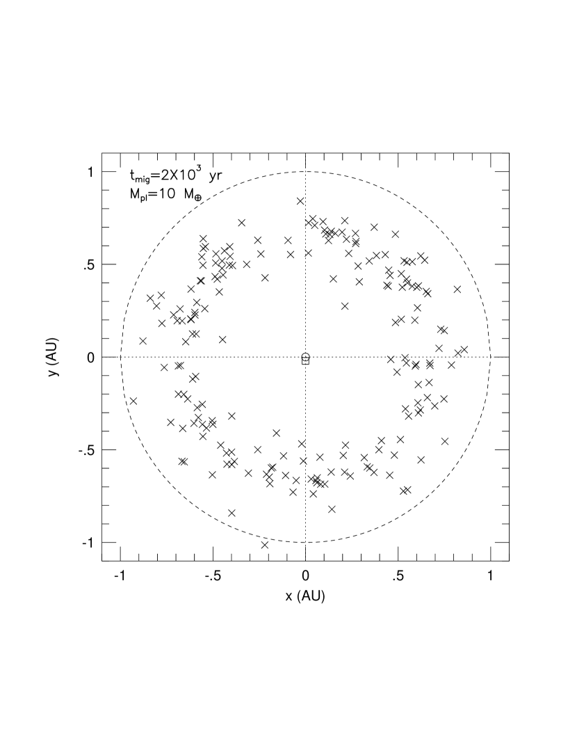
Figure 8.— The final distribution of planetesimals (represented by crosses), in the $x$–$y$ plane in units AU, after a protoplanet of mass 10 M_⊕ has migrated inwards with $t_{mig}=2\times 10^{3}$ yr. The initial protoplanet orbit is indicated by the outer circle (dashed line) and the final one by the very small inner circle (solid line). The protoplanet is represented by the open square. About 23% of the planetesimals were accreted.

Figure 9.— Schematic plot of the fits $\dot{M}_{st}\left(\Sigma\right)$. The solid lines represent a fit of the curves $\log_{10}\left(\dot{M}_{st}\right)$ vs. $\log_{10}\left(\Sigma\right)$ with an arbitrary scale at two different arbitrary radii $r_{1}$ and $r_{2}$ such that $r_{2}>r_{1}$. The dotted line indicates the separation between the optically thin and intermediate regimes.

References

- (1)
- (2) Artymowicz, P. 1994, ApJ, 423, 581
- (3)
- (4) Adams, F. C., Lada, C. J., & Shu, F. H. 1987, ApJ, 312, 788
- (5)
- (6) Balbus, S.A., & Hawley, J. F. 1991, ApJ, 376, 214
- (7)
- (8) Balbus, S.A., & Hawley, J. F. 1998, Rev. Mod. Phys., 70, 1
- (9)
- (10) Beckwith, S. V. W., Sargent, A. I., Chini, R. S., & Guesten, R. 1990, AJ, 99, 924
- (11)
- (12) Beckwith, S. V. W., & Sargent, A. I. 1996, Nature, 383, 139, 144
- (13)
- (14) Bell, K. R., Cassen, P., Klahr, H. H., Henning, T. 1997, ApJ, 486, 372
- (15)
- (16) Bell, K. R., & Lin, D. N. C. 1994, ApJ, 427, 987
- (17)
- (18) Bodenheimer, P. 1998, in Brown dwarfs and extrasolar planets, ed. R. Rebolo, E. L. Martin & M. R. Zapatero Osorio (ASP Conference Series 134), 115
- (19)
- (20) Bodenheimer, P., Hubickyj, O., & Lissauer, J. J. 1998, preprint
- (21)
- (22) Bodenheimer, P., & Pollack, J. B. 1986, Icarus, 67, 391
- (23)
- (24) Boss, A. P. 1998, ApJ, 503, 923
- (25)
- (26) Burrows, C. J. et al. 1996, ApJ, 473, 437
- (27)
- (28) Butler, R. P., Marcy, G. W., Williams, E., Hauser, H., & Shirts, P. 1997, ApJ, 474, L115
- (29)
- (30) Cameron, A. G. W. 1978, Moon Planets, 18, 5
- (31)
- (32) Chabrier, G., Saumon, D., Hubbard, W. B., & Lunine, J. I. 1992, ApJ, 391, 817
- (33)
- (34) Chiang, E. I., & Goldreich, P. 1997, ApJ, 490, 368
- (35)
- (36) Cox, J. P., & Giuli, R. T. 1968, Principles of Stellar Structure: Physical Principles (New York: Gordon & Breach)
- (37)
- (38) Gammie, C. F. 1996, ApJ, 457, 355
- (39)
- (40) Ghosh, P., & Lamb, F. K. 1979, ApJ, 232, 259
- (41)
- (42) Goldreich, P., & Soter, S. 1966, Icarus, 5, 375
- (43)
- (44) Goldreich, P., & Tremaine, S. 1980, ApJ, 241, 425
- (45)
- (46) Hartmann, L., Calvet, N., Gullbring, E., & d’Alessio, P. 1998, ApJ, 495, 385
- (47)
- (48) Kant, I. 1755, Allegmeine Naturgeschichte und Theorie des Himmels (Leipzig)
- (49)
- (50) Kary, D. M. , Lissauer, J. J. , & Greenzweig, Y. 1993, Icarus, 106, 288
- (51)
- (52) Koresko, C. D. 1998, ApJ, 507, L145
- (53)
- (54) Korycansky, D. G. , & Papaloizou, J. C. B. 1996, ApJS, 105, 181
- (55)
- (56) Korycansky, D. G. , & Pollack, J. B. 1993, Icarus, 102, 105
- (57)
- (58) Krist, J. E. et al. 1998, ApJ, 501, 841
- (59)
- (60) Kuiper, G. P. 1951, in Astrophysics, ed. J. A. Hynek (New York: McGraw Hill), 357
- (61)
- (62) Laplace, P. S. 1796, Exposition du Système du Monde (Paris)
- (63)
- (64) Levermore, C. D., & Pomraning, G. C. 1981, ApJ, 262, 768
- (65)
- (66) Lin, D. N. C., Bodenheimer, P., & Richardson, D. C. 1996, Nature, 380, 606
- (67)
- (68) Lin, D. N. C., & Papaloizou, J. C. B. 1979a, MNRAS, 186, 799
- (69)
- (70) Lin, D. N. C., & Papaloizou, J. C. B. 1979b, MNRAS, 188, 191
- (71)
- (72) Lin, D. N. C., & Papaloizou, J. C. B. 1980, MNRAS, 191, 37
- (73)
- (74) Lin, D. N. C., & Papaloizou, J. C. B. 1985, in Protostars and planets II, ed. D. C. Black & M. S. Mathews (Tucson: Univ. Arizona Press), 981
- (75)
- (76) Lin, D. N. C., & Papaloizou, J. C. B. 1986, ApJ, 309, 846
- (77)
- (78) Lin, D. N. C., & Papaloizou, J. C. B. 1993, in Protostars and planets III, ed. E. H. Levy & J. Lunine (Tucson: Univ. Arizona Press), 749
- (79)
- (80) Lin, D. N. C., Papaloizou, J. C. B., Terquem, C., Bryden, G., & Ida, S. 1999, in Protostars and planets IV, ed. A. Boss, V. Mannings & S. Russel (Tucson: Univ. Arizona Press), in press
- (81)
- (82) Lissauer, J. J. 1993, ARA&A, 31, 129
- (83)
- (84) Lissauer, J. J., & Stewart, G. R. 1993, in Protostars and planets III, ed. E. H. Levy & J. Lunine (Tucson: Univ. Arizona Press), 1061
- (85)
- (86) Lynden–Bell, D., & Pringle, J. E. 1974, MNRAS, 168, 60
- (87)
- (88) Marcy, G. W., & Butler, R. P. 1998, ARA&A, 36, 57
- (89)
- (90) McCaughrean, M. J. et al. 1998, ApJ, 492, L157
- (91)
- (92) McCaughrean, M. J., & O’Dell, C. R. 1996, AJ, 111, 1977
- (93)
- (94) Mizuno, H. 1980, Prog. Theor. Phys., 64, 544
- (95)
- (96) Murray, N., Hansen, B., Holman, M., & Tremaine, S. 1998, Science, 279, 69
- (97)
- (98) Papaloizou, J. C. B. , & Lin, D. N. C. 1995, ARA&A, 33, 50
- (99)
- (100) Paatz, G. & Camenzind, M. 1996, A& A, 308, 77
- (101)
- (102) Perri, F., & Cameron, A. G. W. 1974, Icarus, 22, 416
- (103)
- (104) Podolak, M., Hubbard, W. B., & Pollack, J. B. 1993, in Protostars and planets III, ed. E. H. Levy & J. Lunine (Tucson: Univ. Arizona Press), 1109
- (105)
- (106) Pollack, J. B., Hubickyj, O., Bodenheimer, P., Lissauer, J. J., Podolak, M., & Greenzweig, Y. 1996 Icarus, 124, 62
- (107)
- (108) Press, W. H., Flannery, B. P., Teukolsky, S. A., & Vetterling, W. T. 1992, Numerical Recipes: The Art of Scientific Computing (Cambridge: Cambridge Univ. Press), 3rd ed.
- (109)
- (110) Rasio, F. A., & Ford, E. B. 1996, Science, 274, 54
- (111)
- (112) Safronov, V. S. 1969, in Evoliutsiia doplanetnogo oblaka, Moscow
- (113)
- (114) Schwarzschild, M. 1958, Structure and Evolution of the Stars (Princeton: Princeton Univ. Press)
- (115)
- (116) Shakura, N. I., & Sunyaev, R. A. 1973, A&A, 24, 337
- (117)
- (118) Stapelfeldt, K. R., Krist, J. E., Menard, F., Bouvier, J., Padgett, D. L., & Burrows, C. J. 1998, ApJ, 502, 65
- (119)
- (120) Stauffer, J. R., Prosser, C. F., Hartmann, L., & McCaughrean, M. J. 1994, AJ, 108, 1375
- (121)
- (122) Stevenson, D. J. 1982, Plan. Space. Sc., 30, 755
- (123)
- (124) Strom, S. E., Edwards, S., & Skrutskie, M. F. 1993, in Protostars and planets III, ed. E. H. Levy & J. Lunine (Tucson: Univ. Arizona Press), 837
- (125)
- (126) Tanaka, H., & Ida, S. 1997, Icarus, 125, 302
- (127)
- (128) Trilling, D. E., Benz, W., Guillot, T., Lunine, J. I., Hubbard, W. B., Burrows, A. 1998, ApJ, 500, 42
- (129)
- (130) Ward, W. R. 1986, Icarus, 67, 164
- (131)
- (132) Ward, W. R. 1997a, ApJ, 482, L211
- (133)
- (134) Ward, W. R. 1997b, Icarus, 126, 261
- (135)
- (136) Ward, W. R., & Hahn, J. M. 1995, ApJ, 440, L25
- (137)
- (138) Weidenschilling, S. J., & Marzari, F. 1996, Nature, 384, 619
- (139)
- (140) Wetherill, G. W., & Stewart, G. R. 1989, Icarus, 77, 330
- (141)
- (142) Wuchterl, G. 1993, Icarus, 106, 323
- (143)
- (144) Wuchterl, G. 1995, Earth, Moon, and Planets, 67, 51
- (145)