Big Bang Nucleosynthesis UMN-TH-1753/99
TPI-MINN-99/15
astro-ph/9903309
March 1999

Abstract

A brief review of standard big bang nucleosynthesis theory and the related observations of the light element isotopes is presented. Implications of BBN on chemical evolution and constraints on particle properties will also be discussed.

1 INTRODUCTION

The standard model [1, 2, 3] of big bang nucleosynthesis (BBN) is based on the inclusion of an extended nuclear network into a homogeneous and isotropic FRLW cosmology. There is now sufficient data to define the standard model in terms of a single parameter, namely the baryon-to-photon ratio, $\eta$. Other factors, such as the uncertainties in reaction rates, and the neutron mean-life can be treated by standard statistical and Monte Carlo techniques [4, 5, 6] to make predictions (with specified uncertainties) of the abundances of the light elements, D, ³He, ⁴He, and ⁷Li. Even the number of neutrino flavors, $N_{\nu}$, which has long been treated as a parameter can simply be set (=3) in defining the standard model.

In this review, I will compare the predictions of BBN with the available observational determinations of the light element abundances and test for concordance. I will also discuss the implications of these results on the Galactic chemical evolution of the light elements and on limits to particle properties.

1.1 Historical Aside

It is important to bear in mind that there has always been an intimate connection between BBN and the microwave background as a key test to the standard big bang model. Indeed, it was the formulation of BBN which predicted the existence of the microwave background radiation [7]. The argument is rather simple. BBN requires temperatures greater than 100 keV, which according to the standard model time-temperature relation, $t_{\rm s}T^{2}_{\rm MeV}=2.4/\sqrt{N}$, where $N$ is the number of relativistic degrees of freedom at temperature $T$, corresponds to timescales less than about 200 s. The typical cross section for the first link in the nucleosynthetic chain is

$$\sigma v(p+n\rightarrow D+\gamma)\simeq 5\times 10^{-20}{\rm cm}^{3}/{\rm s}$$ (1)

This implies that it was necessary to achieve a density

$$n\sim{1\over\sigma vt}\sim 10^{17}{\rm cm}^{-3}$$ (2)

The density in baryons today is known approximately from the density of visible matter to be ${n_{B}}_{o}\sim 10^{-7}$ cm^-3 and since we know that that the density $n$ scales as $R^{-3}\sim T^{3}$, the temperature today must be

$$T_{o}=({n_{B}}_{o}/n)^{1/3}T_{\rm BBN}\sim 10{\rm K}$$ (3)

thus linking two of the most important tests of the Big Bang theory.

2 THEORY

Conditions for the synthesis of the light elements were attained in the early Universe at temperatures $T\mathrel{\raise 1.29167pt\hbox{$<$\kern-7.5pt\lower 4.30554pt\hbox{$\sim$}}}$ 1 MeV. At somewhat higher temperatures, weak interaction rates were in equilibrium. In particular, the processes

$$n+e^{+} \leftrightarrow p+{\bar{\nu}_{e}}$$

$$n+\nu_{e} \leftrightarrow p+e^{-}$$

$$n \leftrightarrow p+e^{-}+{\bar{\nu}_{e}}$$

fix the ratio of number densities of neutrons to protons. At $T\gg 1$ MeV, $(n/p)\simeq 1$.

As the temperature fell and approached the point where the weak interaction rates were no longer fast enough to maintain equilibrium, the neutron to proton ratio was given approximately by the Boltzmann factor, $(n/p)\simeq e^{-\Delta m/T}$, where $\Delta m$ is the neutron-proton mass difference. The final abundance of ⁴He is very sensitive to the $(n/p)$ ratio

$$Y_{p}={2(n/p)\over\left[1+(n/p)\right]}\approx 0.25$$ (4)

Freeze out occurs at slightly less than an MeV resulting in $(n/p)\sim 1/6$ at this time.

The nucleosynthesis chain begins with the formation of Deuterium through the process, $p+n\rightarrow$ D $+\gamma$. However, because the large number of photons relative to nucleons, $\eta^{-1}=n_{\gamma}/n_{B}\sim 10^{10}$, Deuterium production is delayed past the point where the temperature has fallen below the Deuterium binding energy, $E_{B}=2.2$ MeV (the average photon energy in a blackbody is ${\bar{E}}_{\gamma}\simeq 2.7T$). This is because there are many photons in the exponential tail of the photon energy distribution with energies $E>E_{B}$ despite the fact that the temperature or ${\bar{E}}_{\gamma}$ is less than $E_{B}$. During this delay, the neutron-to-proton ratio drops to $(n/p)\sim 1/7$.

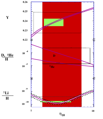
The dominant product of big bang nucleosynthesis is ⁴He resulting in an abundance of close to 25% by mass. Lesser amounts of the other light elements are produced: D and ³He at the level of about $10^{-5}$ by number, and ⁷Li at the level of $10^{-10}$ by number. The resulting abundances of the light elements are shown in Figure 1, which concentrate on the range in $\eta_{10}$ between 1 and 10. The curves for the ⁴He mass fraction, $Y$, bracket the computed range based on the uncertainty of the neutron mean-life which has been taken as $\tau_{n}=887\pm 2$ s. Uncertainties in the produced ⁷Li abundances have been adopted from the results in Hata et al. [5]. Uncertainties in D and ³He production are small on the scale of this figure. The boxes correspond to the observed abundances and will be discussed below.

Figure 1: The light element abundances from big bang nucleosynthesis as a function of $\eta_{10}=10^{10}\eta$.

3 Data

3.1 ⁴He

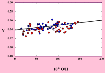
The primordial ⁴He abundance is best determined from observations of HeII $\rightarrow$ HeI recombination lines in extragalactic HII (ionized hydrogen) regions. There is now a good collection of abundance information on the ⁴He mass fraction, $Y$, O/H, and N/H in over 70 [8, 9, 10] such regions. Since ⁴He is produced in stars along with heavier elements such as Oxygen, it is then expected that the primordial abundance of ⁴He can be determined from the intercept of the correlation between $Y$ and O/H, namely $Y_{p}=Y({\rm O/H}\to 0)$. A detailed analysis of the data including that in [10] found an intercept corresponding to a primordial abundance $Y_{p}=0.234\pm 0.002\pm 0.005$ [11]. This was updated to include the most recent results of [12] in [13]. The result (which is used in the discussion below) is

$$Y_{p}=0.238\pm 0.002\pm 0.005$$ (5)

The first uncertainty is purely statistical and the second uncertainty is an estimate of the systematic uncertainty in the primordial abundance determination [11]. The solid box for ⁴He in Figure 1 represents the range (at 2$\sigma_{\rm stat}$) from (5). The dashed box extends this by including the systematic uncertainty. A somewhat lower primordial abundance of $Y_{p}=0.235\pm.003$ is found by restricting to the 36 most metal poor regions [13]. These results are consistent with those of a Bayesian analysis [14] based on the 32 points of lowest metallicity. These have been used to calculate a likelihood function for which the peak occurs at $Y_{p}=0.238$ and the most likely spread is $w=0.009$. The 95% CL upper limit to $Y_{p}$ in this case is 0.245. For further details on this approach see [14].

Figure 2: The ⁴He mass fraction as determined in extragalactic H II regions as a function of O/H.

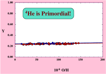
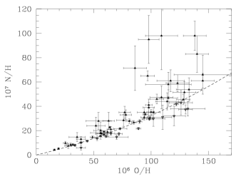
A global view of the ⁴He data is shown in Figure 2. What should be absolutely apparent from this figure is the primordial nature of ⁴He. There are no observations to date which indicate a ⁴He abundance which is significantly below 23% to 24%. In particular, even in systems in which an element such as Oxygen, which traces stellar activity, is observed at extremely low values (compared with the solar value of O/H $\approx 8.5\times 10^{-4}$), the ⁴He abundance is nearly constant. This is far different from all other element abundances (with the exception of ⁷Li as we will see below). For example, in Figure 3, the N/H vs. O/H correlation is shown. As one can clearly see, the abundance of N/H goes to 0, as O/H goes to 0, indicating a stellar source for Nitrogen.

Figure 3: The Nitrogen and Oxygen abundances in the same extragalactic HII regions with observed ⁴He shown in Figure 2.

Figure 4: The Helium (Y) and Oxygen (O/H) abundances in extragalactic HII regions, from refs. [8, 9] and from ref. [12]. Lines connect the same regions observed by different groups. The regression shown leads to the primordial ⁴He abundance given in Eq. (5).

A more useful plot of the ⁴He data is shown in Figure 4. Here one sees the correlation of ⁴He with O/H and the linear regression which leads to primordial abundance given in Eq. (5).

3.2 ⁷Li

The abundance of ⁷Li has been determined by observations of over 100 hot, population-II stars, and is found to have a very nearly uniform abundance [15]. For stars with a surface temperature $T>5500$ K and a metallicity less than about 1/20th solar (so that effects such as stellar convection may not be important), the abundances show little or no dispersion beyond that which is consistent with the errors of individual measurements. Indeed, as detailed in ref. [16, 17], much of the work concerning ⁷Li has to do with the presence or absence of dispersion and whether or not there is in fact some tiny slope to a [Li] = $\log$ ⁷Li/H + 12 vs. T or [Li] vs. [Fe/H] relationship ([Fe/H] is the log of the Fe/H ratio relative to the solar value).

When the Li data from stars with [Fe/H] $<$ -1.3 is plotted as a function of surface temperature, one sees a plateau emerging for $T>5500$ K as shown in Figure 5 for the data taken from ref. [16].

Figure 5: The Li abundance in halo stars with [Fe/H] $<$ -1.3, as a function of surface temperature. The dashed line shows the value of the weighted mean of the plateau data.

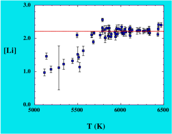
As one can see from the figure, at high temperatures, where the convection zone does not go deep below the surface, the Li abundance is uniform. At lower surface temperatures, the surface abundance of Li is depleted as Li is dragged through the hotter interior of the star and destroyed. The lack of dispersion in the plateau region is evidence that this abundance is indeed primordial (or at least very close to it).

I will use the value given in ref. [16] as the best estimate for the mean ⁷Li abundance and its statistical uncertainty in halo stars

$${\rm Li/H=(1.6\pm 0.1)\times 10^{-10}}$$ (6)

The small error is is statistical and is due to the large number of stars in which ⁷Li has been observed. The solid box for ⁷Li in Figure 1 represents the 2$\sigma_{\rm stat}$ range from (6). There is however an important source of systematic error due to the possibility that Li has been depleted in these stars, though the lack of dispersion in the Li data limits the amount of depletion. In addition, standard stellar models[18] predict that any depletion of ⁷Li would be accompanied by a very severe depletion of ⁶Li. Until recently, ⁶Li had never been observed in hot pop II stars. The observation[19] of ⁶Li (which turns out to be consistent with its origin in cosmic-ray nucleosynthesis) is another good indication that ⁷Li has not been destroyed in these stars [20, 21, 22].

Aside from the big bang, Li is produced together with Be and B in accelerated particle interactions such as cosmic ray spallation of C,N,O by protons and $\alpha$-particles. Li is also produced by $\alpha-\alpha$ fusion. Be and B have been observed in these same pop II stars and in particular there are a dozen or so stars in which both Be and ⁷Li have been observed. Thus Be (and B though there is still a paucity of data) can be used as a consistency check on primordial Li [23]. Based on the Be abundance found in these stars, one can conclude that no more than 10-20% of the ⁷Li is due to cosmic ray nucleosynthesis leaving the remainder (an abundance near $10^{-10}$) as primordial. A similar conclusion was reached in [17]. The dashed box in Figure 1, accounts for the possibility that as much as half of the primordial ⁷Li has been destroyed in stars, and that as much as 20% of the observed ⁷Li may have been produced in cosmic ray collisions rather than in the Big Bang. For ⁷Li, the uncertainties are clearly dominated by systematic effects.

4 Likelihood Analyses

At this point, having established the primordial abundance of at least two of the light elements, ⁴He and ⁷Li, with reasonable certainty, it is possible to test the concordance of BBN theory with observations. Monte Carlo techniques have proven to be a useful form of analysis in this regard [4, 5, 6]. Two elements are sufficient for not only constraining the one parameter theory of BBN, but also for testing for consistency [24]. The procedure begins by establishing likelihood functions for the theory and observations. For example, for ⁴He, the theoretical likelihood function takes the form

$$L_{\rm BBN}(Y,Y_{\rm BBN})=e^{-\left(Y-Y_{\rm BBN}\left(\eta\right)\right)^{2}/2\sigma_{1}^{2}}$$ (7)

where $Y_{\rm BBN}(\eta)$ is the central value for the ⁴He mass fraction produced in the big bang as predicted by the theory at a given value of $\eta$. $\sigma_{1}$ is the uncertainty in that value derived from the Monte Carlo calculations [5] and is a measure of the theoretical uncertainty in the big bang calculation. Similarly one can write down an expression for the observational likelihood function. Assuming Gaussian errors, the likelihood function for the observations would take a form similar to that in (7).

A total likelihood function for each value of $\eta$ is derived by convolving the theoretical and observational distributions, which for ⁴He is given by

$${L^{{}^{4}{\rm He}}}_{\rm total}(\eta)$$

$$=\int dYL_{\rm BBN}\left(Y,Y_{\rm BBN}\left(\eta\right)\right)L_{\rm O}(Y,Y_{\rm O})$$ (8)

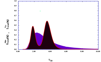
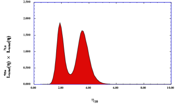
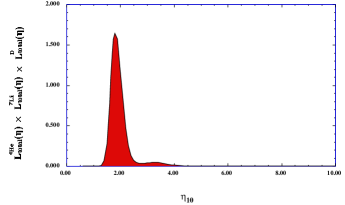
An analogous calculation is performed [24] for ⁷Li. The resulting likelihood functions from the observed abundances given in Eqs. (5) and (6) is shown in Figure 6. As one can see there is very good agreement between ⁴He and ⁷Li in the range of $\eta_{10}\simeq$ 1.5 – 5.0. The double peaked nature of the ⁷Li likelihood function is due to the presence of a minimum in the predicted lithium abundance. For a given observed value of ⁷Li, there are two likely values of $\eta$.

Figure 6: Likelihood distribution for each of ⁴He and ⁷Li, shown as a function of $\eta$. The one-peak structure of the ⁴He curve corresponds to the monotonic increase of $Y_{p}$ with $\eta$, while the two peaks for ⁷Li arise from the minimum in the ⁷Li abundance prediction.

Figure 7: Combined likelihood for simultaneously fitting ⁴He and ⁷Li, as a function of $\eta$.

The combined likelihood, for fitting both elements simultaneously, is given by the product of the two functions in Figure 6 and is shown in Figure 7. The 95% CL region covers the range $1.55<\eta_{10}<4.45$, with the two peaks occurring at $\eta_{10}=1.9$ and 3.5. This range corresponds to values of $\Omega_{B}$ between

$$0.006<\Omega_{B}h^{2}<.016$$ (9)

5 More Data

5.1 D and ³He

Because there are no known astrophysical sites for the production of Deuterium, all observed D is assumed to be primordial. As a result, any firm determination of a Deuterium abundance establishes an upper bound on $\eta$ which is robust.

Deuterium abundance information is available from several astrophysical environments, each corresponding to a different evolutionary epoch. In the ISM, corresponding to the present epoch, an often quoted measurement for D/H is [25]

$${\rm(D/H)_{ISM}}=1.60\pm 0.09{}^{+0.05}_{-0.10}\times 10^{-5}$$ (10)

This measurement allow us to set the upper limit to $\eta_{10}<9$ and is shown by the lower right of the solid box in Figure 1. There are however, serious questions regarding homogeneity of this value in the ISM. There may be evidence for considerable dispersion in D/H [26, 27] as is the case with ³He [28].

The solar abundance of D/H is inferred from two distinct measurements of ³He. The solar wind measurements of ³He as well as the low temperature components of step-wise heating measurements of ³He in meteorites yield the presolar (D + ³He)/H ratio, as D was efficiently burned to ³He in the Sun’s pre-main-sequence phase. These measurements indicate that [29, 30] ${\rm\left({(D+~{}^{3}He)/H}\right)_{\odot}=(4.1\pm 0.6\pm 1.4)\times 10^{-5}}$. The high temperature components in meteorites are believed to yield the true solar ³He/H ratio of [29, 30] ${\rm\left({~{}^{3}He/H}\right)_{\odot}=(1.5\pm 0.2\pm 0.3)\times 10^{-5}}$. The difference between these two abundances reveals the presolar D/H ratio, giving,

$${\rm(D/H)_{\odot}}\approx(2.6\pm 0.6\pm 1.4)\times 10^{-5}$$ (11)

This value for presolar D/H is consistent with measurements of surface abundances of HD on Jupiter D/H = $2.7\pm 0.7\times 10^{-5}$ [31].

Finally, there have been several reported measurements of D/H in high redshift quasar absorption systems. Such measurements are in principle capable of determining the primordial value for D/H and hence $\eta$, because of the strong and monotonic dependence of D/H on $\eta$. However, at present, detections of D/H using quasar absorption systems do not yield a conclusive value for D/H. As such, it should be cautioned that these values may not turn out to represent the true primordial value and it is very unlikely that both are primordial and indicate an inhomogeneity [32] (a large scale inhomogeneity of the magnitude required to placate all observations is excluded by the isotropy of the microwave background radiation). The first of these measurements [33] indicated a rather high D/H ratio, D/H $\approx$ 1.9 – 2.5 $\times 10^{-4}$. Other high D/H ratios were reported in [34]. More recently, a similarly high value of D/H = 2.0 $\pm 0.5\times 10^{-4}$ was reported in a relatively low redshift system (making it less suspect to interloper problems) [35]. This was confirmed in [36] where a 95% CL lower bound to D/H was reported as 8 $\times 10^{-5}$. However, there are reported low values of D/H in other such systems [37] with values of D/H originally reported as low as $\simeq 2.5\times 10^{-5}$, significantly lower than the ones quoted above. The abundance in these systems has been revised upwards to about 3.4 $\pm 0.3\times 10^{-5}$ [38]. However, it was also noted [39] that when using mesoturbulent models to account for the velocity field structure in these systems, the abundance may be somewhat higher (3.5 – 5 $\times 10^{-5}$). This may be quite significant, since at the upper end of this range (5 $\times 10^{-5}$) all of the element abundances are consistent as will be discussed shortly. I will not enter into the debate as to which if any of these observations may be a better representation of the true primordial D/H ratio. The status of these observations are more fully reviewed in [27]. The upper range of quasar absorber D/H is shown by the dashed box in Figure 1.

There are also several types of ³He measurements. As noted above, meteoritic extractions yield a presolar value for ³He/H. In addition, there are several ISM measurements of ³He in galactic HII regions [28] which show a wide dispersion which may be indicative of pollution or a bias [40] ${\rm\left({{}^{3}He/H}\right)_{HII}}\simeq 1-5\times 10^{-5}$. There is also a recent ISM measurement of ³He [41] with ${\rm\left({{}^{3}He/H}\right)_{ISM}}=2.1^{+.9}_{-.8}\times 10^{-5}$. Finally there are observations of ³He in planetary nebulae [42] which show a very high ³He abundance of ³He/H $\sim 10^{-3}$. None of these determinations represent the primordial ³He abundance, and as will be discussed below, their relation to the primordial abundance is heavily dependent on both stellar and chemical evolution.

6 More Analysis

It is interesting to compare the results from the likelihood functions of ⁴He and ⁷Li with that of D/H. Since D and ³He are monotonic functions of $\eta$, a prediction for $\eta$, based on ⁴He and ⁷Li, can be turned into a prediction for D and ³He. The corresponding 95% CL ranges are D/H $=(4.1-25)\times 10^{-5}$ and ³He/H $=(1.2-2.6)\times 10^{-5}$. If we did have full confidence in the measured value of D/H in quasar absorption systems, then we could perform the same statistical analysis using ⁴He, ⁷Li, and D. To include D/H, one would proceed in much the same way as with the other two light elements. We compute likelihood functions for the BBN predictions as in Eq. (7) and the likelihood function for the observations. These are then convolved as in Eq. (8).

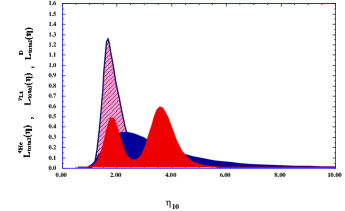
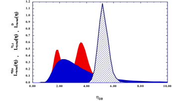
Using D/H = $(2.0\pm 0.5)\times 10^{-4}$ as indicated in the high D/H systems, we can plot the three likelihood functions including $L^{{\rm D}}_{\rm total}(\eta)$ in Figure 8. It is indeed startling how the three peaks, for D, ⁴He and ⁷Li are in excellent agreement with each other. In Figure 9, the combined distribution is shown. We now have a very clean distribution and prediction for $\eta$, $\eta_{10}=1.8^{+1.6}_{-.3}$ corresponding to $\Omega_{B}h^{2}=.007^{+.005}_{-.001}$. The absence of any overlap with the high-$\eta$ peak of the ⁷Li distribution has considerably lowered the upper limit to $\eta$. Overall, the concordance limits in this case are dominated by the Deuterium likelihood function.

Figure 8: As in Figure 6, with the addition of the likelihood distribution for D/H assuming “high” D/H.

Figure 9: Combined likelihood for simultaneously fitting ⁴He and ⁷Li, and D as a function of $\eta$ from Figure 8.

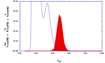
If instead, we assume that the low value [38] of D/H = $(3.4\pm 0.3)\times 10^{-5}$ is the primordial abundance, then we can again compare the likelihood distributions as in Figure 8, now substituting the low D/H value. As one can see from Figure 10, there is now hardly any overlap between the D and the ⁷Li and ⁴He distributions. The combined distribution shown in Figure 11 is compared with that in Figure 9. In this case, D/H is just compatible (at the 2 $\sigma$ level) with the other light elements, and the peak of the likelihood function occurs at $\eta_{10}=4.8^{+0.5}_{-0.6}$. Though one can not use this likelihood analysis to prove the correctness of the high D/H measurements or the incorrectness of the low D/H measurements, the analysis clearly shows the difference in compatibility between the two values of D/H and the observational determinations of ⁴He and ⁷Li. To make the low D/H measurement compatible, one would have to argue for a shift upwards in ⁴He to a primordial value of 0.247 (a shift by 0.009) which is not warranted at this time by the data, and a ⁷Li depletion factor of about 2, which is close to recent upper limits to the amount of depletion [43, 21].

Figure 10: As in Figure 8, with the likelihood distribution for low D/H.

Figure 11: Combined likelihood for simultaneously fitting ⁴He and ⁷Li, and low D/H as a function of $\eta$. The dashed curve represents the combined distribution shown in Figure 9.

It is important to recall however, that the true uncertainty in the low D/H systems might be somewhat larger. If we allow D/H to be as large as $5\times 10^{-5}$, the peak of the D/H likelihood function shifts down to $\eta_{10}\simeq 4$. In this case, there would be a near perfect overlap with the high $\eta$ ⁷Li peak and since the ⁴He distribution function is very broad, this would be a highly compatible solution.

7 Chemical Evolution

Because we can not directly measure the primordial abundances of any of the light element isotopes, we are required to make some assumptions concerning the evolution of these isotopes. As has been discussed above, ⁴He is produced in stars along with Oxygen and Nitrogen. ⁷Li can be destroyed in stars and produced in several (though still uncertain) environments. D is totally destroyed in the star formation process and ³He is both produced and destroyed in stars with fairly uncertain yields. It is therefore preferable, if possible to observe the light element isotopes in a low metallicity environment. Such is the case with ⁴He and ⁷Li. These elements are observed in environments which are as low as 1/50th and 1/1000th solar metallicity respectively and we can be fairly assured that the abundance determinations of these isotopes are close to primordial. If the quasar absorption system measurements of D/H stabilize, then this too may be very close to a primordial measurement. Otherwise, to match the solar and present abundances of D and ³He to their primordial values requires a model of galactic chemical evolution.

The main inputs to chemical evolution models are: 1) The initial mass function, $\phi(m)$, indicating the distribution of stellar masses. Typically, a simple power law form for the IMF is chosen, $\phi(m)\sim m^{-x}$, with $x\simeq-2.7$. This is a fairly good representation of the observed distribution, particularly at larger masses. 2) The star formation rate, $\psi$. Typical choices for a SFR are $\psi(t)\propto\sigma$ or $\sigma^{2}$ or even a straight exponential $e^{-t/\tau}$. $\sigma$ is the fraction of mass in gas, $M_{\rm gas}/M_{\rm tot}$. 3) The presence of infalling or outflowing gas; and of course 4) the stellar yields. It is the latter, particularly in the case of ³He, that is the cause for so much uncertainty. Chemical evolution models simply set up a series of evolution equations which trace desired quantities.

Deuterium is always a monotonically decreasing function of time in chemical evolution models. The degree to which D is destroyed, is however a model dependent question which depends sensitively on the IMF and SFR. The evolution of ³He is however considerably more complicated. Stellar models predict that substantial amounts of ³He are produced in stars between 1 and 3 M_⊙. For example, in the models of Iben and Truran [44] a 1 M_⊙ star will yield a ³He abundance which is nearly three times as large as its initial (D+³He) abundance. It should be emphasized that this prediction is in fact consistent with the observation of high ³He/H in planetary nebulae [42].

However, the implementation of standard model ³He yields in chemical evolution models leads to an overproduction of ³He/H particularly at the solar epoch [40, 45]. While the overproduction is problematic for any initial value of D/H, it is particularly bad in models with a high primordial D/H. In Scully et al. [46], a dynamically generated supernovae wind model was coupled to models of galactic chemical evolution with the aim of reducing a primordial D/H abundance of 2 $\times 10^{-4}$ to the present ISM value without overproducing heavy elements and remaining consistent with the other observational constraints typically imposed on such models. In Figure 12, the evolution of D/H and ³He/H is shown as a function of time in one of the models with significant Deuterium destruction factors (see ref [46] for details). While such a model can successfully account for the evolution of D/H (and other standard chemical evolution tracers), as one can plainly see, ³He is grossly overproduced (the Deuterium data is represented by squares and ³He by circles).

Figure 12: The evolution of D/H and ³He/H with time in units of $10^{-5}$. The assumed primordial abundance of D/H is 2 $\times 10^{-4}$. The dashed ³He curve shows the evolution with standard ³He yields, while the solid curve shows the effect of the reduced yields of [48].

The overproduction of ³He relative to the solar meteoritic value seems to be a generic feature of chemical evolution models when ³He production in low mass stars is included. This result appears to be independent of the chemical evolution model and is directly related to the assumed stellar yields of ³He. It has recently been suggested that at least some low mass stars may indeed be net destroyers of ³He if one includes the effects of extra mixing below the conventional convection zone in low mass stars on the red giant branch [47, 48]. The extra mixing does not take place for stars which do not undergo a Helium core flash (i.e. stars $>$ 1.7 - 2 M_⊙ ). Thus stars with masses less than 1.7 M_⊙ are responsible for the ³He destruction. Using the yields of Boothroyd and Malaney [48], it was shown [49] that these reduced ³He yields in low mass stars can account for the relatively low solar and present day ³He/H abundances observed. In fact, in some cases, ³He was underproduced. To account for the ³He evolution and the fact that some low mass stars must be producers of ³He as indicated by the planetary nebulae data, it was suggested that the new yields apply only to a fraction (albeit large) of low mass stars [49, 50]. The corresponding evolution [49] of D/H and ³He/H using the reduced yields is shown in Figure 12.

The models of chemical evolution discussed above indicate that it is possible to destroy significant amounts of Deuterium and remain consistent with chemical evolutionary constraints. To do so however, comes with a price. Large Deuterium destruction factors require substantial amounts of stellar processing, which at the same time produce heavy elements. To keep the heavy element abundances in the Galaxy in check, significant Galactic winds enriched in heavy elements must be incorporated. In fact there is some evidence that enriched winds were operative in the early Galaxy. In the X-ray cluster satellites observed by Mushotzky et al. [51] and Loewenstein and Mushotzky [52] the mean Oxygen abundance was found to be roughly half solar. This corresponds to a near solar abundance of heavy elements in the inter-Galactic medium, where apparently little or no star formation has taken place.

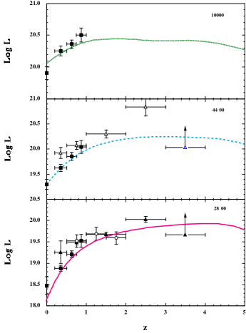
If our Galaxy is typical in the Universe, then the models of the type discussed above would indicate that the luminosity density of the Universe at high redshift should also be substantial augmented relative to the present. Recent observations of the luminosity density at high redshift [53] are making it possible for the first time to test models of cosmic chemical evolution. The high redshift observations, are very discriminatory with respect to a given SFR [54]. Models in which the star formation rate is proportional to the gas mass fraction (these are common place in Galactic chemical evolution) have difficulties to fit the multi-color data from $z=0$ to 1. This includes many of the successful Galactic infall models. In contrast, models with a steeply decreasing SFR are favored. In Figure 13, the predicted luminosity density based on the model with evolution shown in Figure 12 from [46], as compared with the observations (see ref. [54] for details).

Figure 13: The tricolor luminosity densities (UV, B and IR) at $\lambda=0.28,0.44$ and 1.0 $\mu$m, in units of (h/.5) WHz^-1Mpc^-3 as a function of redshift for a model shown in 12 which destroys significant amounts of D/H. The data are taken from [53].

While it would be premature to conclude that all models with large Deuterium destruction factors are favored, it does seem that models which do fit the high redshift data destroy significant amounts of D/H. On the other hand, we can not exclude models which destroy only a small amount of D/H as Galactic models of chemical evolution. In this case, however the evolution of our Galaxy is anomalous with respect to the cosmic average. If the low D/H measurements [37, 38] hold up, then it would seem that our Galaxy also has an anomalously high D/H abundance. That is we would predict in this case that the present cosmic abundance of D/H is significantly lower than the observed ISM value. (This conclusion assumes that the ISM D/H abundance is representative of the present epoch. If new results [26] which show values as low as a few $\times 10^{-6}$ are more typical, then low primordial D/H would fit the high redshift data and models with a high degree of D destruction much better.) If the high D/H observations [33, 34, 35] hold up, we could conclude that our Galaxy is indeed representative of the cosmic star formation history.

8 Constraints from BBN

Limits on particle physics beyond the standard model are mostly sensitive to the bounds imposed on the ⁴He abundance. As is well known, the ⁴He abundance is predominantly determined by the neutron-to-proton ratio just prior to nucleosynthesis and is easily estimated assuming that all neutrons are incorporated into ⁴He. As discussed earlier, the neutron-to-proton ratio is fixed by its equilibrium value at the freeze-out of the weak interaction rates at a temperature $T_{f}\sim 1$ MeV modulo the occasional free neutron decay. Furthermore, freeze-out is determined by the competition between the weak interaction rates and the expansion rate of the Universe

$${G_{F}}^{2}{T_{f}}^{5}\sim\Gamma_{\rm wk}(T_{f})=H(T_{f})\sim\sqrt{G_{N}N}{T_{f}}^{2}$$ (12)

where $N$ counts the total (equivalent) number of relativistic particle species. The presence of additional neutrino flavors (or any other relativistic species) at the time of nucleosynthesis increases the overall energy density of the Universe and hence the expansion rate leading to a larger value of $T_{f}$, $(n/p)$, and ultimately $Y_{p}$. Because of the form of Eq. (12) it is clear that just as one can place limits [55] on $N$, any changes in the weak or gravitational coupling constants can be similarly constrained (for a recent discussion see ref. [56]).

As discussed above, the limit on $N_{\nu}$ comes about via the change in the expansion rate given by the Hubble parameter,

$$H^{2}={8\pi G\over 3}\rho={8\pi^{3}G\over 90}[N_{\rm SM}+{7\over 8}\Delta N_{\nu}]T^{4}$$ (13)

when compared to the weak interaction rates. Here $N_{\rm SM}$ refers to the standard model value for N. At $T\sim 1$ MeV, $N_{\rm SM}=43/4$. Additional degrees of freedom will lead to an increase in the freeze-out temperature eventually leading to a higher ⁴He abundance. In fact, one can parameterize the dependence of $Y$ on $N_{\nu}$ by

$$Y=0.2262+0.0131(N_{\nu}-3)+0.0135\ln\eta_{10}$$ (14)

in the vicinity of $\eta_{10}\sim 2$. Eq. (14) also shows the weak (log) dependence on $\eta$. However, rather than use (14) to obtain a limit, it is preferable to use the likelihood method.

Just as ⁴He and ⁷Li were sufficient to determine a value for $\eta$, a limit on $N_{\nu}$ can be obtained as well [24, 57, 58, 6]. The likelihood approach utilized above can be extended to include $N_{\nu}$ as a free parameter. Since the light element abundances can be computed as functions of both $\eta$ and $N_{\nu}$, the likelihood function can be defined by [57] replacing the quantity $Y_{\rm BBN}\left(\eta\right)$ in eq. (7) with $Y_{\rm BBN}\left(\eta,N_{\nu}\right)$ to obtain ${L^{{}^{4}{\rm He}}}_{\rm total}(\eta,N_{\nu})$. Again, similar expressions are needed for ⁷Li and D.

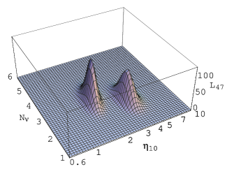
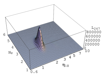
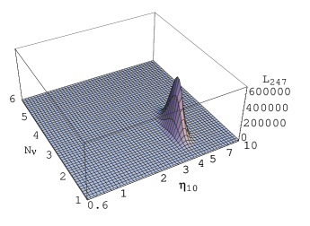
A three-dimensional view of the combined likelihood functions [58] is shown in Figure 14. In this case the high and low $\eta$ maxima of Figure 7, show up as peaks in the $L-\eta-N_{\nu}$ space. The likelihood function is labeled $L_{47}$ (and $L_{247}$ when D/H is included). In Figures 15 and 16 the corresponding likelihood functions $L_{247}$ with high and low D/H are shown. Once again one sees an effect of including D/H is to eliminate one of the ⁷Li peaks. Furthermore, unlike the case discussed in section 6, the likelihood distribution for low D/H is just as strong as that for high D/H, albeit at a lower value of $N_{\nu}$.

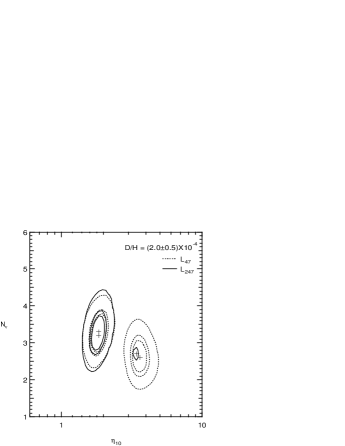
The peaks of the distribution as well as the allowed ranges of $\eta$ and $N_{\nu}$ are more easily discerned in the contour plots of Figures 17 and 18 which show the 50%, 68% and 95% confidence level contours in $L_{47}$ and $L_{247}$ for high and low D/H as indicated. The crosses show the location of the peaks of the likelihood functions. $L_{47}$ peaks at $N_{\nu}=3.2$, $\eta_{10}=1.85$ and at $N_{\nu}=2.6$, $\eta_{10}=3.6$. The 95% confidence level allows the following ranges in $\eta$ and $N_{\nu}$

$$1.7\leq N_{\nu}\leq 4.3\qquad\qquad 1.4\leq\eta_{10}\leq 4.9$$ (15)

Note however that the ranges in $\eta$ and $N_{\nu}$ are strongly correlated as is evident in Figure 17.

With high D/H, $L_{247}$ peaks at $N_{\nu}=3.3$, and also at $\eta_{10}=1.85$. In this case the 95% contour gives the ranges

$$2.2\leq N_{\nu}\leq 4.4\qquad\qquad 1.4\leq\eta_{10}\leq 2.4$$ (16)

Note that within the 95% CL range, there is also a small area with $\eta_{10}=3.2-3.5$ and $N_{\nu}=2.5-2.9$.

Similarly, for low D/H, $L_{247}$ peaks at $N_{\nu}=2.4$, and $\eta_{10}=4.55$. The 95% CL upper limit is now $N_{\nu}<3.2$, and the range for $\eta$ is $3.9<\eta_{10}<5.4$. It is important to stress that with the increase in the determined value of D/H [38] in the low D/H systems, these abundances are now consistent with the standard model value of $N_{\nu}=3$ at the 2 $\sigma$ level.

Figure 14: $L_{47}(N_{\nu},\eta)$ for observed abundances given by eqs. (5 and 6).

Figure 15: $L_{247}(N_{\nu},\eta)$ for observed abundances including high D/H.

Figure 16: $L_{247}(N_{\nu},\eta)$ for observed abundances including low D/H.

Figure 17: 50%, 68% & 95% C.L. contours of $L_{47}$ and $L_{247}$ where observed abundances are given by eqs. (5 and 6), and high D/H.

Figure 18: 50%, 68% & 95% C.L. contours of $L_{47}$ and $L_{247}$ where observed abundances are given by eqs. (5 and 6), and low D/H.

9 Summary

To summarize, I would assert that one can conclude that the present data on the abundances of the light element isotopes are consistent with the standard model of big bang nucleosynthesis. Using the isotopes with the best data, ⁴He and ⁷Li, it is possible to constrain the theory and obtain a best set of values for the baryon-to-photon ratio of $\eta_{10}$ and the corresponding value for $\Omega_{B}h^{2}$

$$\begin{array}[]{ccccc}1.55&<&\eta_{10}&<&4.45\qquad 95\%{\rm CL}\\ .006&<&\Omega_{B}h^{2}&<&.016\qquad 95\%{\rm CL}\end{array}$$

For $0.4<h<1$, we have a range $.006<\Omega_{B}<.10$. This is a rather low value for the baryon density and would suggest that much of the galactic dark matter is non-baryonic [60]. These predictions are in addition consistent with recent observations of D/H in quasar absorption systems which show a high value. Difficulty remains however, in matching the solar ³He abundance, suggesting a problem with our current understanding of galactic chemical evolution or the stellar evolution of low mass stars as they pertain to ³He.

This work was supported in part by DoE grant DE-FG02-94ER-40823 at the University of Minnesota.

References

- [1] T.P. Walker, G. Steigman, D.N. Schramm, K.A. Olive and K. Kang, Ap.J. 376 (1991) 51.
- [2] S. Sarkar, Rep. Prog. Phys. 59 (1996) 1493.
- [3] K.A. Olive and D.N. Schramm, Eur.Phys.J. C3 (1998) 119; K.A. Olive, astro-ph/9901231.
- [4] L.M. Krauss and P. Romanelli, Ap.J. 358 (1990) 47; L.M. Krauss and P.J. Kernan, Phys. Lett. B347 (1995) 347; M. Smith, L. Kawano, and R.A. Malaney, Ap.J. Supp. 85 (1993) 219; P.J. Kernan and L.M. Krauss, Phys. Rev. Lett. 72 (1994) 3309.
- [5] N. Hata, R.J. Scherrer, G. Steigman, D. Thomas, and T.P. Walker, Ap.J. 458 (1996) 637.
- [6] G. Fiorentini, E. Lisi, S. Sarkar, and F.L. Villante, Phys.Rev. D58 (1998) 063506.
- [7] G. Gamow, Phys. Rev. 74 (1948) 505; G. Gamow, Nature 162 (1948) 680; R.A. Alpher and R.C. Herman, Nature 162 (1948) 774; R.A. Alpher and R.C. Herman, Phys. Rev. 75 (1949) 1089.
- [8] B.E.J. Pagel, E.A. Simonson, R.J. Terlevich and M. Edmunds, MNRAS 255 (1992) 325.
- [9] E. Skillman and R.C. Kennicutt, Ap.J. 411 (1993) 655; E. Skillman, R.J. Terlevich, R.C. Kennicutt, D.R. Garnett, and E. Terlevich, Ap.J. 431 (1994) 172.
- [10] Y.I. Izotov, T.X. Thuan, and V.A. Lipovetsky, Ap.J. 435 (1994) 647; Ap.J.S. 108 (1997) 1.
- [11] K.A. Olive, E. Skillman, and G. Steigman, Ap.J. 483 (1997) 788.
- [12] Y.I. Izotov, and T.X. Thuan, Ap.J. 500 (1998) 188.
- [13] B.D. Fields and K.A. Olive, Ap.J. 506 (1998) 177.
- [14] C.J. Hogan, K.A. Olive, and S.T. Scully, Ap.J. 489 (1997) L119.
- [15] F. Spite, and M. Spite, A.A. 115 (1982) 357; M. Spite, J.P. Maillard, and F. Spite, A.A. 141 (1984) 56; F. Spite, and M. Spite, A.A. 163 (1986) 140; L.M. Hobbs, and D.K. Duncan, Ap.J. 317 (1987) 796; R. Rebolo, P. Molaro, J.E. and Beckman, A.A. 192 (1988) 192; M. Spite, F. Spite, R.C. Peterson, and F.H. Chaffee Jr., A.A. 172 (1987) L9; R. Rebolo, J.E. Beckman, and P. Molaro, A.A. 172 (1987) L17; L.M. Hobbs, and C. Pilachowski, Ap.J. 326 (1988) L23; L.M. Hobbs, and J.A. Thorburn, Ap.J. 375 (1991) 116; J.A. Thorburn, Ap.J. 399 (1992) L83; C.A. Pilachowski, C. Sneden,and J. Booth, Ap.J. 407 (1993) 699; L. Hobbs, and J. Thorburn, Ap.J. 428 (1994) L25; J.A. Thorburn, and T.C. Beers, Ap.J. 404 (1993) L13; F. Spite, and M. Spite, A.A. 279 (1993) L9. J.E. Norris, S.G. Ryan, and G.S. Stringfellow, Ap.J. 423 (1994) 386; J. Thorburn, Ap.J. 421 (1994) 318.
- [16] P. Molaro, F. Primas, and P. Bonifacio, A.A. 295 (1995) L47; P. Bonifacio and P. Molaro, MNRAS 285 (1997) 847.
- [17] S.G. Ryan, J.E. Norris, and T.C. Beers, astro-ph/9903059.
- [18] C.P. Deliyannis, P. Demarque, and S.D. Kawaler, Ap.J.Supp. 73 (1990) 21.
- [19] V.V. Smith, D.L. Lambert, and P.E. Nissen, Ap.J. 408 (1992) 262; Ap.J. 506 (1998) 405; L. Hobbs, and J. Thorburn, Ap.J. 428 (1994) L25; Ap.J. 491 (1997) 772; R. Cayrel, M. Spite, F. Spite, E. Vangioni-Flam, M. Cassé, and J. Audouze, astro-ph/9901205.
- [20] G. Steigman, B. Fields, K.A. Olive, D.N. Schramm, and T.P. Walker, Ap.J. 415 (1993) L35; M. Lemoine, D.N. Schramm, J.W. Truran, and C.J. Copi, Ap.J. 478 (1997) 554.
- [21] M.H. Pinsonneault, T.P. Walker, G. Steigman, and V.K. Naranyanan, Ap.J. (1998) submitted.
- [22] B.D.Fields and K.A. Olive, New Astronomy, astro-ph/9811183, in press; E. Vangioni-Flam, M. Cassé, R. Cayrel, J. Audouze, M. Spite, and F. Spite, New Astronomy, astro-ph/9811327, in press.
- [23] T.P. Walker, G. Steigman, D.N. Schramm, K.A. Olive and B. Fields, Ap.J. 413 (1993) 562; K.A. Olive, and D.N. Schramm, Nature 360 (1993) 439.
- [24] B.D. Fields and K.A. Olive, Phys. Lett. B368 (1996) 103; B.D. Fields, K. Kainulainen, D. Thomas, and K.A. Olive, New Astronomy 1 (1996) 77.
- [25] J.L. Linsky, et al., Ap.J. 402 (1993) 694; J.L. Linsky, et al.,Ap.J. 451 (1995) 335.
- [26] E.B. Jenskins, T.M. Tripp, P.R. Wozniak, U.J. Sofia, and G. Sonneborn, astro-ph/9901403.
- [27] A. Vidal-Madjar, these proceedings
- [28] D.S. Balser, T.M. Bania, C.J. Brockway, R.T. Rood, and T.L. Wilson, Ap.J. 430 (1994) 667; T.M. Bania, D.S. Balser, R.T. Rood, T.L. Wilson, and T.J. Wilson, Ap.J.S. 113 (1997) 353.
- [29] S.T. Scully, M. Cassé, K.A. Olive, D.N. Schramm, J.W. Truran, and E. Vangioni-Flam, Ap.J. 462 (1996) 960.
- [30] J. Geiss, in Origin and Evolution of the Elements, eds. N. Prantzos, E. Vangioni-Flam, and M. Cassé (Cambridge: Cambridge University Press, 1993), p. 89.
- [31] H.B. Niemann, et al. Science 272 (1996) 846; P.R. Mahaffy, T.M. Donahue, S.K. Atreya, T.C. Owen, and H.B. Niemann, Sp. Sci. Rev. 84 (1998) 251.
- [32] C. Copi, K.A. Olive, and D.N. Schramm, Proc. Nat. Ac. Sci. 95 (1998) 2758, astro-ph/9606156.
- [33] R.F. Carswell, M. Rauch, R.J. Weymann, A.J. Cooke, and J.K. Webb, MNRAS 268 (1994) L1; A. Songaila, L.L. Cowie, C. Hogan, and M. Rugers, Nature 368 (1994) 599.
- [34] M. Rugers and C.J. Hogan, A.J. 111 (1996) 2135; R.F. Carswell, et al. MNRAS 278 (1996) 518; E.J. Wampler, et al., A.A. 316 (1996) 33.
- [35] J.K. Webb, R.F. Carswell, K.M. Lanzetta, R. Ferlet, M. Lemoine, A. Vidal-Madjar, and D.V. Bowen, Nature 388 (1997) 250.
- [36] D. Tytler, S. Burles, L. Lu, X.-M. Fan, A. Wolfe, and B.D. Savage, astro-ph/9810217.
- [37] D. Tytler, X.-M. Fan, and S. Burles, Nature 381 (1996) 207; S. Burles and D. Tytler, Ap.J. 460 (1996) 584.
- [38] S. Burles and D. Tytler, Ap.J. 499 (1998) 699; Ap.J. 507 (1998) 732.
- [39] S. Levshakov, D. Tytler, and S. Burles, astro-ph/9812114.
- [40] K.A. Olive, R.T. Rood, D.N. Schramm, J.W. Truran, and E. Vangioni-Flam, Ap.J. 444 (1995) 680.
- [41] G. Gloeckler, and J. Geiss, Nature 381 (1996) 210.
- [42] R.T. Rood, T.M. Bania, and T.L. Wilson, Nature 355 (1992) 618; R.T. Rood, T.M. Bania, T.L. Wilson, and D.S. Balser, 1995, in the Light Element Abundances, Proceedings of the ESO/EIPC Workshop, ed. P. Crane, (Berlin:Springer), p. 201; D.S. Balser, T.M. Bania, R.T. Rood, T.L. Wilson, Ap.J. 483 (1997) 320.
- [43] S. Vauclair and C. Charbonnel, A.A. 295 (1995) 715.
- [44] I. Iben, and J.W. Truran, Ap.J. 220 (1978) 980.
- [45] D. Galli, F. Palla, F. Ferrini, and U. Penco, Ap.J. 443 (1995) 536; D. Dearborn, G. Steigman, and M. Tosi, Ap.J. 465 (1996) 887.
- [46] S. Scully, M. Cassé, K.A. Olive, and E. Vangioni-Flam, Ap.J. 476 (1997) 521.
- [47] C. Charbonnel, A. A. 282 (1994) 811; C. Charbonnel, Ap.J. 453 (1995) L41; C.J. Hogan, Ap.J. 441 (1995) L17; G.J. Wasserburg, A.I. Boothroyd, andI.-J. Sackmann, Ap.J. 447 (1995) L37; A. Weiss, J. Wagenhuber, and P. Denissenkov, A.A. 313 (1996) 581.
- [48] A.I. Boothroyd, A.I. and R.A. Malaney, astro-ph/9512133.
- [49] K.A. Olive, D.N. Schramm, S. Scully, and J.W. Truran, Ap.J. 479 (1997) 752.
- [50] D. Galli, L. Stanghellini, M. Tosi, and F. Palla Ap.J. 477 (1997) 218.
- [51] R. Mushotzky, et al., Ap.J. 466 (1996) 686
- [52] M. Loewenstein and R. Mushotzky, Ap.J. 466 (1996) 695.
- [53] S.J. Lilly, O. Le Fevre, F. Hammer, and D. Crampton, ApJ 460 (1996) L1; P. Madau, H.C. Ferguson, M.E. Dickenson, M. Giavalisco, C.C. Steidel, and A. Fruchter, MNRAS 283 (1996) 1388; A.J. Connolly, A.S. Szalay, M. Dickenson, M.U. SubbaRao, and R.J. Brunner, ApJ 486 (1997) L11; M.J. Sawicki, H. Lin, and H.K.C. Yee, A.J. 113 (1997) 1.
- [54] M. Cassé, K.A. Olive, E. Vangioni-Flam, and J. Audouze, New Astronomy 3 (1998) 259.
- [55] G. Steigman, D.N. Schramm, and J. Gunn, Phys. Lett. B66 (1977) 202.
- [56] B.A. Campbell and K.A. Olive, Phys. Lett. B345 (1995) 429; L. Bergstrom, S. Iguri, and H. Rubinstein. astro-ph/9902157.
- [57] K.A. Olive and D. Thomas, Astro. Part. Phys. 7 (1997) 27.
- [58] K.A. Olive and D. Thomas, Astro. Part. Phys. (in press), hep-ph/9811444.
- [59] G. Steigman, K.A. Olive, and D.N. Schramm, Phys. Rev. Lett. 43 (1979) 239; K.A. Olive, D.N. Schramm, and G. Steigman, Nucl. Phys. B180 (1981) 497.
- [60] E. Vangioni-Flam and M. Cassé, Ap.J. 441 (1995) 471.