Cosmic microwave background map making with data between 10 and 90 GHz

Abstract

We use data from the Tenerife 10, 15 and 33 GHz beamswitching experiments along with the COBE 53 and 90 GHz data to separate the cosmic microwave background (CMB) signal from the Galactic signal and create two maps at high Galactic latitude. The new multi-MEM technique is used to obtain the best reconstruction of the two channels. The two maps are presented and known features are identified within each. We find that the Galactic contribution to both the 15 and 33 GHz Tenerife data is small enough to be ignored when compared to the errors in the data and the magnitude of the CMB signal.

1 Introduction

When analysing data from cosmic microwave background (CMB) experiments it is important to be able to distinguish features originating from the CMB and those that originate from foregrounds. With the sensitivity of experiments improving it is becoming increasingly important to subtract these foregrounds from the data before any cosmological interpretation is made. Using multi-frequency observations it should be possible to extract information on both the CMB and foregrounds sources.

The multi-maximum entropy method (multi-MEM) can be used to analyse multi-frequency observations to obtain constraints on the various foregrounds that affect CMB experiments. Hobson et al. (1998) use this method to analyse simulated data from the Planck satellite experiment and Jones et al. (1999a) apply it to simulated data from the MAP satellite. In applying this technique the different frequency observations must be sensitive to the same structures (i.e. they have an overlapping window function) as well as observing the same region.

Fortunately the Tenerife beam-switching experiments have an overlapping window function and common observing region with the COBE satellite. This constitutes a region with a frequency range of 10 GHz to 90 GHz and, therefore, offers enough data to allow Galactic subtraction from CMB data. We present the results of this joint analysis in the form of a CMB map and Galactic foreground map at 10 GHz.

2 Tenerife data

The observing strategy and telescope design of the Tenerife experiments have been described elsewhere (see Gutierrez et al. 1995 and references therein). The data to be used in the analysis here have been presented in a companion paper (Gutierrez et al. 1999) and consist of scans at constant declination from a set of beam-switching experiments. To make use of a large range in frequency coverage it is only possible to use the data between Declinations $32.5\nobreak^{\circ}$ and $42.5\nobreak^{\circ}$ where there is data at both 10 GHz and 15 GHz. The Declination strips are separated by $2.5\nobreak^{\circ}$ and so there are 5 scans in the final analysis (it is noted that the technique described below does not require the same number of declinations at each frequency but as we require a Galactic separation we are limited by our coverage at the lowest frequency where the Galactic emission dominates). We also concentrate our analysis at high Galactic latitudes away from strong Galactic emission (RA $160\nobreak^{\circ}-260\nobreak^{\circ}$) where the CMB signal will be more dominant). The final stacked data scans consist of continuous observations binned in $1\nobreak^{\circ}$ intervals in Right Ascension (RA) and the final average noise per bin is $130\mu$K at 10 GHz and $54\mu$K at 15 GHz (corresponding to $50\mu$K and $20\mu$K per beam respectively). The beamwidths are $4.9\nobreak^{\circ}$ and $5.2\nobreak^{\circ}$ FWHM at 10 GHz and 15 GHz, respectively. We also include the 33 GHz ($5.0\nobreak^{\circ}$ FWHM and $55\mu$K error per bin), Dec. $40\nobreak^{\circ}$ Tenerife data that was presented in Hancock et al. (1994) as an extra constraint. No other data at this frequency is currently available.

3 COBE data

The COBE satellite window function overlaps that of the Tenerife window function (Watson et al. 1992) and so it should see the same features. The sensitivity of the four-year COBE data is also comparable to that of the Tenerife data and so it forms a useful constraint on the level of CMB, relative to the Galactic emission, contained in the two data sets. We extract the region overlapping that observed by the Tenerife 10 GHz experiment at high Galactic latitude (RA $160-260\nobreak^{\circ}$, Dec. $32.5-42.5\nobreak^{\circ}$) which corresponds to 200 COBE pixels at each frequency. As the noise in the 30 GHz COBE channel is much larger than that in the other two channels (53 GHz and 90 GHz) and also much larger than in the Tenerife data we opt not to use this data in the analysis. Our final data set therefore consists of data covering RA $160-260\nobreak^{\circ}$, Dec. $32.5-42.5\nobreak^{\circ}$ at 10, 15, 33, 53 and 90 GHz covering almost an order of magnitude in frequency.

4 Multi-MEM analysis technique

The multi-MEM technique has been presented elsewhere (Hobson et al. 1998). Here we will only outline the implementation of the technique to the data set considered in this paper. As has been previously shown (Jones et al. 1998) the Tenerife data set contains long term baseline variations which can be simultaneously subtracted from the data when applying the MEM technique. This is still done with the multi-MEM technique and the only difference between the single channel MEM presented in Jones et al. (1998) and the multi-MEM technique considered here is that the $\chi^{2}$ is now a sum over each of the frequency channels and the entropy is a sum over each of the reconstructed maps (in this case the CMB and Galactic foreground maps). The information that the multi-MEM technique requires is only the frequency spectra of the channels to be reconstructed (although this can be relaxed if a search over spectral indices is performed as in Section 5.1). The maximum entropy result was found using a Newton-Raphson iteration method until convergence was obtained (usually about 120 iterations were used although convergence was reached within $\sim 60$ iterations).

4.1 The choice of $\alpha$ and $m$

The choice of the Bayesian parameter $\alpha$ and the model parameter $m$ in the Maximum Entropy method have often been treated as a ‘guesswork’. In Fourier space it is possible to calculate the Bayesian value for the $\alpha$ parameter but in real space this becomes much more complicated as it involves the inversion of large matrices (see Hobson et al. 1998). In the past $m$ was chosen to be the rms of the signal expected in the reconstruction and $\alpha$ was chosen so that the final value of $F=\chi^{2}-\alpha S$ was approximately equal to the number of data points, $N$. Actually $F$ was chosen to be just below $N+2\sqrt{N}$ which is the confidence limit on $F$ calculated by using the degrees of freedom on $\chi^{2}$ as a function of the reconstruction. Here we investigate the behaviour of the Monte-Carlo reconstructions with varying $\alpha$ and $m$ and show that this approximation is actually a very good one. Figures 1 and 2 show the variation of $F$ with $\alpha$ and $m$ respectively. Also shown is the average error on the reconstructions. As is seen the minimum in the errors on the reconstruction for $\alpha$ occurs when $F$ is within the allowed range for classic MEM ($F=N\pm 2\sqrt{N}$ where $N$ is the number of data points). The minimum value for $F$ when varying $m$ occurs where $m=50\mu$K which is the rms of the expected reconstruction. Therefore, our initial ‘guesses’ at $\alpha$ and $m$ are properly justified and are the values used in the following analysis.

Figure 1: The thin line shows $F=\chi^{2}-\alpha S$ as a function of the Bayesian parameter $\alpha$. The classical allowed range for $F$ is given between the two dotted lines (see text). The thick line shows the error on the reconstruction as a function of $\alpha$. Each point was calculated over 50 Monte-Carlo simulations.

Figure 2: The thin line shows $F=\chi^{2}-\alpha S$ as a function of the model parameter $m$. The classical allowed range for $F$ is given between the two dotted lines (see text). The thick line shows the error on the reconstruction as a function of $m$. Each point was calculated over 50 Monte-Carlo simulations.

5 Application to the data

The multi-MEM technique was applied to the full Tenerife and COBE data set assuming that there were two sources for the fluctuations seen in the data. The spectral dependencies of these two sources were that of CMB and that of free-free emission (although this was later relaxed, see Section 5.1). Simultaneous long term baseline removal was performed on the Tenerife maps and any features with a period longer than $25\nobreak^{\circ}$ (corresponding to features that are outside the Tenerife window function) were subtracted. The convergence of the MEM algorithm is shown in Figure 3.

Figure 3: $\chi^{2}-\alpha S$ per pixel as a function of the number of iterations of the Newton-Raphson minimisation process. It is seen that the MEM algorithm converges very rapidly and approaches the classic MEM result as required ($\chi^{2}-\alpha S=N$ where $N$ is the number of pixels).

Figure 4 shows the CMB reconstruction obtained and Figure 5 shows the Galactic foreground reconstruction. As can be seen the two maps clearly have different features. The sky coverage is limited by the smallest survey (10 GHz) although the single declination at 33 GHz (Dec. $40\nobreak^{\circ}$) is included in the analysis as an extra constraint. The rms signal at 10 GHZ for the CMB and Galactic maps are $42\mu$K and $36\mu$K respectively. Taking a free-free spectral index this corresponds to a Galactic signal of $15\mu$K at 15 GHz and $3\mu$K at 33 GHz which implies that the Galactic foreground is negligable in both cases (when added in quadrature). The error on the CMB and Galactic reconstruction is $40\mu$K and $30\mu$K per $1\nobreak^{\circ}$ pixel respectively (compared with errors of $46\mu$K and $35\mu$K on the reconstructions of the separate 10 GHz and 15 GHz channels respectively presented in Gutierrez et al. 1999). This error was calculated from the variance over 300 Monte-Carlo simulations of the MEM analysis. The reconstruction contains individual features at $5\nobreak^{\circ}$ resolution (the maximum resolution of the Tenerife experiments) and the error over one of these features is therefore $\sim 9\mu$K for the CMB map and $\sim 7\mu$K for the Galactic map.

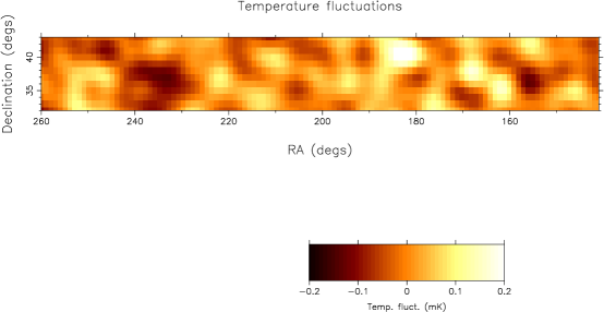
Figure 4: The reconstructed CMB map at 10 GHz. The region shown here corresponds to the high Galactic latitude region used by the Tenerife group as it is relatively low in Galactic contamination (at 10 GHz the signal from the CMB and Galaxy are roughly equal on $5\nobreak^{\circ}$ scales). The error on this reconstruction is $40\mu$K per $1\nobreak^{\circ}$ square pixel or $9\mu$K per $5\nobreak^{\circ}$ feature.

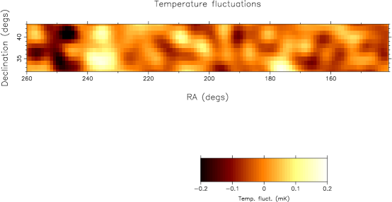
Figure 5: The reconstructed Galactic map at 10 GHz. The region is the same as Figure 4. The error on this reconstruction is $30\mu$K per $1\nobreak^{\circ}$ square pixel or $7\mu$K per $5\nobreak^{\circ}$ feature.

5.1 Spectral index determination

The analysis performed assumed that the Galactic foreground was free-free emission with a temperature spectral index of -2.1. Clearly, this is an assumption which may be incorrect as the dominant foreground in this region could be from another source. Therefore, it is necessary to vary this spectral index to see how the foreground and CMB reconstructions change. This has been done over a range for the spectral index of 0.0 to -4.0. Figure 6 shows the variation in $\chi^{2}$ (comparing the predicted data to the real data) over this range of spectral index. As can be seen there is a broad minimum above a spectral index of $\sim 2$ which implies that in this range very little is changed in the two reconstructions. This is because the main information on the Galactic channel occurs in the 10 GHz data and the higher frequency data acts as upper limits. Therefore, it appears as though the Galactic foreground fits the data well with a spectral index of $\sim 2$ which corresponds to free-free emission (this spectral index corresponds to the point at which the Galactic contribution at the higher frequencies is just below the upper limit). Changes in the CMB reconstruction were well below the noise when the spectral index was varied for the Galactic channel.

6 Identification of features

The main purpose of using the multi-MEM technique is to allow clean separation of CMB sources from foreground emission. This can be checked by comparing the two maps with existing surveys and previous predictions.

It is very difficult to compare the features in the maps with known Galactic features as very few surveys at similar frequencies and scale cover the Tenerife region of sky. However, there is a survey at 5 GHz which uses an interferometer and has been used to create a map of Galactic fluctuations covering this region (Jones et al. 1999b, hereafter JB98). Also, the 408 MHz (Haslam, Salter, Stoffel & Wilson 1982) and 1420 MHz (Reich & Reich 1988) surveys cover this region but the artefacts within the 1420 MHz survey makes a meaningful comparison difficult (JB98). By comparison with the survey presented in JB98 some common features are observed. For example, the Galactic feature at RA $175\nobreak^{\circ}$, Dec. $32.5\nobreak^{\circ}$ was seen in the 5 GHz and the 408 MHz survey. The point source at Dec. $30\nobreak^{\circ}$, RA $200\nobreak^{\circ}$ appeared to be extended in the 5 GHz survey and there appears to be a Galactic feature in the same region which could account for this extension. However, there are features which appear in the Galactic map here and not in the lower frequency surveys although this could be due to the different angular scale dependencies. For example, there is a large feature at RA $230\nobreak^{\circ}$, Dec. $35\nobreak^{\circ}-40\nobreak^{\circ}$. This only shows up in the 5 GHz map at very small amplitude and this could be due to the interferometer resolving out the feature. This feature was observed at Dec. $40\nobreak^{\circ}$ in an $8\nobreak^{\circ}$ FWHM beam at 10 GHz using the predecessor to the Tenerife experiments (Davies et al 1987).

The CMB map is even more difficult to compare with other maps as the only two surveys which have covered this region are the COBE and Tenerife experiments. Therefore, no comparison is possible at this time although it is possible to check previous predictions made by the COBE and Tenerife teams. The main predictions about the CMB were the feature at Dec. $40\nobreak^{\circ}$, RA $185\nobreak^{\circ}$ (Hancock et al. 1994) and the positive-negative-positive feature (smoothed to $10\nobreak^{\circ}$ scale in RA) at Dec. $35\nobreak^{\circ}$, RA. $200-250\nobreak^{\circ}$ (Bunn, Hoffman & Silk, 1996 and Gutierrez et al. 1997), both of which are clearly seen here (the second being a combination of negative and positive fluctuations). The other features in this map are all potentially CMB in origin but must wait until other experiments with overlapping window functions have surveyed this region before being assigned unambiguously.

Figure 6: $\chi^{2}$ as a function of the input spectral index ($T\propto\nu^{-\beta}$) of the Galactic channel. A spectral index of 2.1 corresponds to free-free emission.

7 Conclusions and further work

The reconstructed maps using data between 10 GHz and 90 GHz were presented. Features of Galactic and cosmological origin were identified. The CMB map is very similar to the reconstructed map using the 15 GHz Tenerife data alone (Gutierrez et al. 1999) and so it is possible to use that data alone as a constraint on the CMB to put limits on the cosmological parameters as has been done in the past. It was found that the Galactic contamination in this frequency range is consistent with free-free emission (if the upper limit set by the 15 GHz data is a true limit), although no constraint on the relative level of free-free and synchrotron emission was possible. Taking all of the Galactic foreground to be free-free emission it was found that the 15 GHz data was contaminated by $15\pm 3\mu$K which is very small when added in quadrature to the CMB signal of $42\pm 9\mu$K. If the foreground was all synchrotron emission then this value would be even lower. At 33 GHz the free-free component would contribute a signal of $3.0\pm 0.6\mu$K which is negligible.

There are many future applications of this technique. The multi-MEM has been applied to simulated Planck and MAP satellite data already. We are presently collating other CMB and Galactic surveys together to put further constraints on the foregrounds and the CMB itself at different angular scales and covering a wider frequency range to reduce the errors obtained here. The only constraint that this method has on producing real CMB maps is that there is enough frequency coverage of experiments with over lapping window functions that observe the same region of sky. We are also combining data from experiments with different window functions to put direct constraints on the spatial power spectrum of the CMB and Galactic fluctuations. We are currently working on applying this technique to the spherical sky and a full likelihood analysis, as well as tests for non-Gaussianity within the data, will be presented soon.

References

- [1] Bunn, E.F., Hoffman, Y., & Silk, J. 1996, ApJ, 464, 1
- [2] Davies, R.D., Lasenby, A.N., Watson, R.A., Daintree, E.J., Hopkins, J., Beckman, J.E., Sanchez-Almeida, J. & Rebolo, R. 1987, Nature, 326, 462
- [3] Gutierrez, C.M., Rebolo, R., Watson, R., Davies, R.D., Jones, A.W. & Lasenby, A.N. 1999, ApJ, submitted
- [4] Gutierrez, C. M., Hancock, S., Davies, R. D., Rebolo, R., Watson, R. A., Hoyland, R.J., Lasenby, A. N. & Jones A.W. 1997, ApJ, 480, L83
- [5] Gutierrez, C.M., Davies, R.D., Rebolo, R., Watson, R.A., Hancock, S. & Lasenby, A.N. 1995, ApJ, 442, 10
- [6] Hancock, S. et al. 1994, Nature, 367, 333
- [7] Haslam, C.G.T., Salter, C.J., Stoffel, H., & Wilson, W.E. 1982, A&AS, 47, 1
- [8] Hobson, M.P., Jones, A.W., Lasenby, A.N. & Bouchet, F. 1998, MNRAS, 300, 1
- [9] Jones, A.W., Hancock, S., Lasenby, A.N., Davies, R.D., Gutierrez, C.M., Rocha, G., Watson, R.A., & Rebolo, R. 1998, MNRAS, 294, 582
- [10] Jones, A.W., Hobson, M.P. & Lasenby, A.N. 1999a, MNRAS, in press
- [11] Jones, A.W., Wilkinson, A., Giardino, G., Melhuish, S., Asareh, H., Davies, R.D. & Lasenby, A.N. 1999b, (JB99), MNRAS, submitted
- [12] Reich, P., & Reich, W. 1988, A&AS, 74, 7
- [13] Watson, R.A., Gutierrez, C.M., Davies, R.D., Lasenby, A.N., Rebolo, R., Beckman, J.E. & Hancock, S. 1992, Nature, 357, 660