Probing early-type galaxy evolution with the Kormendy relation

Abstract

We investigate the evolution of early-type galaxies in four clusters at $z=0.4$ (Abell 370, Cl 0303$+$17, Cl 0939$+$47 and Cl 1447$+$26) and in one at $z=0.55$ (Cl 0016$+$16). The galaxies are selected according to their spectrophotometrically determined spectral types and comprise the morphological classes E, S0 and Sa galaxies. Structural parameters are determined by a two-component fitting of the surface brightness profiles derived from HST images. Exploring a realistic range of K-corrections using Bruzual and Charlot models, we construct the rest-frame $B$-band Kormendy relations ($\mathrm{\langle\-\mu_{e}}\rangle-\log(R_{e})$) for the different clusters. We do not detect a systematic change of the slope of the relation as a function of redshift. We discuss in detail how the luminosity evolution, derived by comparing the Kormendy relations of the distant clusters with the local one for Coma, depends on various assumptions and give a full description of random and systematic errors by exploring the influences of selection bias, different star formation histories and K-corrections.

Early-type galaxies with modest disk components (S0 and Sa) do not differ significantly in their evolution from disk-less ellipticals.

The observed luminosity evolution is compatible with pure passive evolution models (with redshift of formation $z>2$) but also with models that allow ongoing star formation on a low level, like exponentially decaying star formation models with an e-folding time of $\tau=1$ Gyr.

1 Introduction

In the past years, many observations have been made to investigate the redshift evolution of elliptical galaxies and to compare them with stellar population synthesis models. Most of the authors conclude that the stellar populations in cluster ellipticals evolve mainly in a passive manner (Bower et al., 1992; Aragón-Salamanca et al., 1993; Rakos and Schombert, 1995; Barger et al., 1996; Bender et al., 1996; Ellis et al., 1997; Stanford et al., 1998; Ziegler and Bender, 1997, and others). Passive evolution models assume a short but intensive initial star formation phase and no subsequent star formation Bruzual and Charlot (1993). Other studies have shown that most of the observations are also compatible with hierarchical evolution models Kauffmann (1996); Kauffmann and Charlot (1998). One of the most accurate tools to test galaxy evolution is offered by the scaling relations which hold for elliptical galaxies, like the Fundamental Plane Djorgovski and Davis (1987); Dressler et al. (1987). Here we write the Fundamental Plane equation in a form where the mean effective surface brightness $\mathrm{\langle\mu_{e}\rangle}$ is given as a function of effective radius $R_{e}$ (in kpc) and velocity dispersion $\sigma$:

$$\mathrm{\langle\mu_{e}\rangle}=\tilde{a}+\tilde{b}\cdot\log R_{e}+c\cdot\log\sigma$$ (1)

First observations of the Fundamental Plane at intermediate redshifts indicate indeed the passive evolution of elliptical cluster galaxies van Dokkum and Franx (1996); Kelson et al. (1997); Jørgensen and Hjorth (1997); Bender et al. (1998); van Dokkum et al. (1998).

The determination of the Fundamental Plane parameters at even modest redshifts is non-trivial and requires good signal-to-noise ratios. The velocity dispersion can only be derived from intermediate-resolution spectra obtained with either 8m-class telescopes or very long exposure times at 4m class telescopes Ziegler and Bender (1997); Kelson et al. (1997). Because the galaxy size is of order of a few arcsec at $z>0.2$, the structural parameters can be measured accurately only in the spatially highly resolved Hubble Space Telescope images. With WFPC2 delivering such images now in great numbers, but lacking the spectroscopic information, many studies have been made exploiting the projection of the Fundamental Plane onto the plane defined by $R_{e}$ and $\mathrm{\langle\mu_{e}\rangle}$, i.e. the Kormendy relation Kormendy (1977):

$$\mathrm{\langle\mu_{e}\rangle}=a+b\cdot\log R_{e}$$ (2)

This relation was used to perform the Tolman test for the cosmological dependence of the surface brightness assuming passive luminosity evolution for elliptical galaxies Pahre et al. (1996); Moles et al. (1998). While the first group finds the $(1+z)^{4}$ dependence of the surface brightness in an expanding Universe confirmed, the second group points out that the scatter in the observed data is too large to significantly constrain any cosmological model. Other groups utilized the Kormendy relation to investigate the luminosity evolution itself both for field galaxies Schade et al. (1996); Fasano et al. (1998) and for cluster galaxies Barrientos et al. (1996); Schade et al. (1997); Barger et al. (1998). All these studies conclude that the evolution of the stellar populations in spheroidal galaxies is most probably purely passive at low redshifts ($z\la 0.6$) and that their formation epoch lies at high redshift ($z_{f}>2$).

Most of the cited studies have however the disadvantage that they must rely on photometry only, so that neither cluster membership of a galaxy is guaranteed, nor that the sample is not contaminated by some post-starburst galaxies like E$+$A galaxies. The early-type galaxies are also not distinguished with respect to E or S0 types. All the authors assume a fixed slope $b$ of the Kormendy relation, although its validity at any redshift is not proven a priori. The errors in the transformation from HST magnitudes into the photometric system of the local reference system are not always taken into account in the derivation of the luminosity evolution. All these points are addressed in this paper. We start our investigations of spectrophotometrically defined early-type member galaxies in five distant clusters (Sect. 2) with a thorough analysis of the possible systematic errors arising from the magnitude calibration (Sect. 3). After examining the coefficients of the Kormendy relation of some representative local samples, we determine its slope in the distant clusters by a free bisector fit and derive the luminosity evolution by comparison with one specific local cluster sample. Then, we fit all the cluster samples with the same slope for the Kormendy relation and study the difference in the derived evolution (Sect. 4). The influence of a number of parameters is investigated in Sect. 5. We also look at the results for subsamples containing only galaxies with and without a substantial disk component, and for the whole sample augmented by a few known E$+$A galaxies. Finally, we investigate which evolutionary models (not only the passive one) can fit the data within their errors (Sect. 6). In the appendix, we present the photometric parameters of all the galaxies in the distant clusters studied here.

2 The sample and parameter determination

In this paper we examine the early-type galaxy population in four clusters at redshifts around $z=0.4$ (Abell 370, Cl 0303$+$17, Cl 0939$+$47 and Cl 1447$+$26) and one at $z=0.55$ (Cl 0016$+$16). From ground-based spectrophotometry we determined cluster membership and spectral type of the galaxies, whereas HST images were used to derive morphological and structural parameters.

With the exception of Abell 370, all clusters were observed at the 3.5m telescope of the Calar Alto Observatory. Images were taken in the broad-band filters $B$, $R$ and $I$ and in eight different narrow-band filters, which were chosen to sample characteristic features of galaxy spectra taking into account the clusters’ redshifts. From the multi-band imaging, low resolution spectral energy distributions were constructed which were fitted by template spectra of local galaxy types Coleman et al. (1980). Special care was taken to find post-starburst (E$+$A) galaxies. Their existence was revealed by a good fit of their SED by one of six different model spectra synthesized by the superposition of an elliptical and a burst component. In this manner, cluster membership could be determined with good accuracy and galaxies were classified as either early-type (ET), spiral (Sbc or Scd), irregular (Im) or post-starburst (E$+$A) (Belloni et al., 1995; Belloni and Röser, 1996; Vuletić, 1996; Belloni et al., 1997b, where numerous SED fitting examples can be found). Thus, galaxies were selected according to spectral type and, in the following study, only cluster members of type ET were included. Morphologically, these galaxies could be either E, S0 or Sa galaxies. In the case of Abell 370, we include only spectroscopically confirmed ET member galaxies Mellier et al. (1988); Pickles and van der Kruit (1991); Ziegler and Bender (1997).

HST-WFPC2 $R$ images do exist of the cores of the clusters Abell 370, Cl 1447$+$26, Cl 0939$+$47 and Cl 0303$+$17, whereas Cl 0016$+$16 was observed both in $V$ and $I$ (see Table 1). Additionally, an outer region of Abell 370 and of Cl 0939$+$47 was observed in $V$ and $I$, too. As expected from the density-morphology relation Dressler (1980); Dressler et al. (1997), only a small number of ET galaxies are found in the outer fields, whereas the core images contain 30 to 40 ET galaxies of our ground-based sample. Due to the uncertainties affecting the photometric calibration (see Sect. 3), we did not combine the $V$ and $I$ data of the same galaxies transformed to $B_{\mathrm{r}est}$, and we exclude from our statistical investigation those samples which have less than 10 galaxies.

With the exception of Abell 370, the WFPC2 images were retrieved from the ST/ECF archive as re-processed frames using up to date reduction files. In the case of Abell 370, our original HST data of the core of the cluster were used. The individual images per filter were combined using the imshift and crrej tasks within the IRAF stsdas package STScI (1995). The candidate galaxies were then extracted, stars and artifacts removed, a sky value assigned and the surface-brightness profile fitted Flechsig (1997) within MIDAS ESO (1994). The profile analysis followed the prescription described by Saglia et al. Saglia et al. (1997). In short, a PSF (computed using the Tinytim program) broadened $r^{1/4}$ and an exponential component were fitted simultaneously and separately to the circularly averaged surface brightness profiles. The quality of the fits were explored by Monte Carlo simulations, taking into account sky-subtraction corrections, the signal-to-noise ratio, the radial extent of the profiles and the $\chi^{2}$ quality of the fit. In this way, we were able to detect the disk of lenticular S0 and Sa galaxies and larger disky ellipticals and to derive not only the global values of the total magnitude $M_{\mathrm{tot}}$ and the effective radius $r_{e}$ (in arcsec), but also the luminosity and scale of the bulge ($m_{b}$ and $r_{e,b}$) and disk ($m_{d}$ and $h$) component separately, within the limitations described by Saglia et al. (Saglia et al., 1997, especially Fig. 13). Extensive tests have been made in that paper and it was shown that the fits have only problems with nearly edge-on galaxies. Since all the investigated galaxies have low ellipticities, the deviations around $\log R_{e}-0.3\langle\mu_{e}\rangle$, which is nearly parallel to the Kormendy relation, are minimal. The average error in $M_{\mathrm{tot}}$ is $0.15\,\mathrm{mag}$ and $25\%$ in $r_{e}$. All the photometric parameters of each galaxy are given in the Tables of the Appendix, although only the global values were used to construct the Kormendy relations. Galaxies with $r_{e}<0.25\,\arcsec$ were rejected from our sample because in this case only 5 or less pixels would contribute to the bulge. The number of early-type galaxies (ET) of the different clusters in the observed filters remaining for our investigations are listed in Table 1.

The samples are therefore characterized by a conservative selection, because we pick up all E, S0 and Sa galaxies. However, having derived the disk-to-bulge ratios for the clusters’ galaxies, in a second step we analyze subsamples of objects with $d/b\leq 0.2$ (called E in the following) and $d/b>0.2$ (called S0, but could include also Sa).

Table 1: The sample. Col. 1: cluster name used here, Col. 2: HST filter, Cols. 3 – 5: number of galaxies, Col. 6: $B_{\mathrm{tot}}$ magnitude cut-off, Col. 7: absolute $B$ magnitude limit ($H_{0}=60\,\mathrm{km\,s^{-1}\,Mpc^{-1}},q_{0}=0.1$), Cols. 8 – 10: minimum, median and maximum of the $\log R_{e}$ distribution.

cluster	filter	E,S0,Sa	S0,Sa	E$+$A	$B_{\mathrm{lim}}$	$M_{B,\mathrm{lim}}$	Min($\log R_{e}$)	Med($\log R_{e}$)	Max($\log R_{e}$)
					$\mathrm{mag}$	$\mathrm{mag}$	$R_{e}$ in $\mathrm{kpc}$	$R_{e}$ in $\mathrm{kpc}$	$R_{e}$ in $\mathrm{kpc}$
ComaSBD	B	39	14	0	16.55	$-$18.77	0.04	0.41	1.55
a370v	F555W	9	1	0	20.87	$-$20.82	0.44	0.63	0.92
a370r	F675W	17	8	2	21.25	$-$20.44	0.33	0.67	1.71
a370i	F814W	9	3	0	21.32	$-$20.37	0.43	0.56	0.89
cl1447r	F702W	31	11	2	22.35	$-$19.43	0.21	0.42	1.07
cl0939v	F555W	8	2	3	22.19	$-$19.70	0.28	0.52	0.58
cl0939r	F702W	26	16	9	23.22	$-$18.67	0.19	0.42	1.13
cl0939i	F814W	6	2	2	22.33	$-$19.56	0.25	0.48	0.61
cl0303r	F702W	24	10	6	22.20	$-$19.75	0.19	0.53	1.13
cl0016v	F555W	30	7	7	22.13	$-$20.52	0.27	0.49	1.40
cl0016i	F814W	28	9	3	22.54	$-$20.11	0.27	0.51	1.38

3 Calibration of the data

The mean effective surface brightness $\mathrm{\langle\mu_{e}\rangle_{i}}$ within the (global) effective radius $r_{e}$ for a given HST filter ($i=V,R,I$) is defined as (cf. with Eq. (9) of Holtzman et al. Holtzman et al. (1995)):

$$\mathrm{\langle\mu_{e}\rangle_{i}}=-2.5\log\left(I(<r_{e})/\pi r_{e}^{2}\right)+\mathrm{ZP_{i}(color)},$$ (3)

where $I(<r_{e})$ is the measured flux inside an aperture of radius $r_{e}$:

$$\langle\mu_{e}\rangle_{i}= - 2.5\log(\mathrm{counts})+2.5\log t+2.5\log\mathrm{GR}$$ (4)

$$+ 2.5\log(\pi)+5\log r_{e}+\mathrm{ZP_{i}(color)}$$

We use a gain ratio of GR $=2.0$ for all WFPC2 chips, since the differences between the chips result in magnitude differences which are much smaller than the other systematic errors. To be able to compare the HST data of the distant galaxies with local samples we transform the HST magnitudes into the standard Johnson-Cousins photometric system, in which most ground-based studies are accomplished. For the transformation between WFPC2 magnitudes and UBVRI, there exist two systems, the ‘flight system’ and the ‘synthetic system’ Holtzman et al. (1995). The ‘flight system’ is based on measurements of standard stars with colors $(V-I)<1.5$, whereas the ‘synthetic system’ is calculated from an atlas of stellar spectra. Since elliptical galaxies have colors redder than the stars used for the calibration of the ’flight system’, we rely on the ‘synthetic system’. It is worth noticing that there are systematic differences between the two systems in the overlapping color range. As shown in Fig. 1 these differences are small: $\Delta m\leq 0.005,0.02,0.01$ $\mathrm{mag}$ for the F814W, F675W, F555W filter, respectively. In Table 2, we quote the zeropoints ZP₁ for an exposure time of 1s for colors $(V-R)=1.25$ (F675W and F702W) and $(V-I)=2.2$ (F555W and F814W). The errors refer to variations in colors within the ranges $1.0\leq(V-R)\leq 1.5$ and $1.8\leq(V-I)\leq 2.6$, which are appropriate for early type galaxies. The zeropoints ZP_t for the relevant exposure times $t$ (GR is already included in both ZP) as well as the total integration time $t_{\mathrm{t}ot}$ are also given. We notice that $t$ is the integration time of both a single exposure and of the median image as constructed by the task crrej (old version), whereas $t_{\mathrm{t}ot}$ is the sum of all individual exposures. The ZP are calculated using the coefficients of Table 10 of Holtzman et al. Holtzman et al. (1995). We checked the ZP of Abell 370 by comparing the HST growth curves of eight galaxies to those obtained with NTT data Ziegler (1999) and find agreement within $\approx 0.01\,\mathrm{mag}$. The ZPs of the Calar Alto data of the other clusters are not determined to better than $\approx 0.02\,\mathrm{mag}$.

Table 2: Calibration of $\mathrm{\langle\mu_{e}\rangle}$. Col. 1: cluster name used here, Col. 2: HST filter, Col. 3: redshift, Col. 4: zeropoint for 1s exposure, the error is the maximum deviation of ZP in the assumed color range of the galaxies, Col. 5: exposure time of individual HST frames, Col. 6: ZP for this exposure time, Col. 7: total integration time, Cols. 8. & 9.: reddening, Cols. 10. & 11.: extinction, Col. 12: mean K-correction and maximum deviations for our model SEDs.

cluster	filter	z	ZP1	t	ZPt	$t_{\mathrm{t}ot}$	$E_{(B-V)}$	$E_{(B-V)}$	$A_{i}$	$A_{i}$	$K(B,i)$
							BH	SFD	RL	SFD
Coma	B	0.024					0.0103	0.0089	0.042	0.038	$0.12\pm 0.02$
a370v	F555W	0.375	$22.41\pm 0.01$	1000	29.91	8000	0.0122	0.0384	0.038	0.127	$-0.25\pm 0.05$
a370r	F675W	0.375	$22.08\pm 0.02$	†		5600	0.0122	0.0384	0.028	0.103	$1.02\pm 0.04$
a370i	F814W	0.375	$21.54\pm 0.00$	2100	29.84	12600	0.0122	0.0384	0.018	0.074	$1.88\pm 0.08$
cl1447r	F702W	0.389	$22.74\pm 0.07$	2200	31.11	4200	0.0202	0.0340	0.047	0.091	$1.00\pm 0.02$
cl0939v	F555W	0.407	$22.41\pm 0.01$	1000	29.91	8000	0.0042	0.0164	0.013	0.054	$-0.39\pm 0.06$
cl0939r	F702W	0.407	$22.74\pm 0.07$	2100	31.05	21000	0.0042	0.0164	0.010	0.044	$0.95\pm 0.03$
cl0939i	F814W	0.407	$21.54\pm 0.00$	2100	29.84	10500	0.0042	0.0164	0.006	0.032	$1.84\pm 0.06$
cl0303r	F702W	0.416	$22.74\pm 0.07$	2100	31.05	12600	0.0892	0.1326	0.206	0.354	$0.93\pm 0.02$
cl0016v	F555W	0.55	$22.41\pm 0.01$	2100	30.72	12600	0.0232	0.0572	0.072	0.190	$-0.93\pm 0.09$
cl0016i	F814W	0.55	$21.54\pm 0.00$	2100	29.84	16800	0.0232	0.0572	0.035	0.111	$1.62\pm 0.05$

^† The exposure times of the individual frames of a370r have not a single value.

Figure 1: Transformation between HST-WFPC2 filter magnitudes and Johnson-Cousins filter magnitudes. Zeropoints (ZP) on the left y-axis are calculated according to Table 10 of Holtzman et al. (including the gain ratio of $0.753$ $\mathrm{mag}$), $\Delta$ZP on the right y-axis is the offset from the minimum ZP. Dashed lines correspond to the ‘flight system’ (FS), solid lines to the ‘synthetic system’ (SS). In the case of the F555W filter, FS zeropoints are given as a function of $(V-I)$ color (lower x-axis) and $(V-R)$ color (upper x-axis), respectively, and x-axes zeropoints are shifted in order to match the same typical galaxy colors on a vertical line.

In order to be able to compare the data of the clusters, which are at different redshifts and have been observed in different filters, all observed magnitudes are converted to restframe $B$ magnitudes and corrected for the cosmological dimming of the surface brightness. In addition to applying the K-corrections ($K$), the galactic extinction ($A$) in the respective band ($i=V,R$ or $I$) has to be subtracted:

$$\mathrm{\langle\mu_{e}\rangle}_{B}=\mathrm{\langle\mu_{e}\rangle}_{i}-A_{i}+K(B,i,z)$$ (5)

$$\mathrm{\langle\mu_{e}\rangle_{cor}}=\mathrm{\langle\mu_{e}\rangle}_{B}-10\log(1+z)$$ (6)

There are two major sources for reddening values of the Galaxy in the literature: one is based on H i measurements (Burstein and Heiles, 1984, BH), the other on COBE/DIRBE and IRAS/ISSA FIR data (Schlegel et al., 1998, SFD). Because there are systematic differences, in Table 2 we list $E(B-V)$ values derived from both methods. For the conversion from $E(B-V)$ into $A_{i}$ there exist different interstellar extinction laws in the literature. In Table 2, the extinction is calculated once using the law by Rieke and Lebofsky (Rieke and Lebofsky, 1985, RL) (according to their Table 3) and BH reddenings, and a second time using SFD reddenings according to their extinction curve (their Table 6, Landolt filters). The absorption coefficients $A_{i}$ derived from SFD are systematically larger by about $0.06$ $\mathrm{mag}$ (up to $0.15$ $\mathrm{mag}$) with respect to those derived with the other prescriptions.

The K-correction is defined as the quantity necessary in the case of redshifted objects to convert the observed magnitude in a given filter to the restframe magnitude. With increasing redshift, the restframe $B$ magnitude maps successively into the $V,R$ and $I$ bands. As a consequence, there exist different redshift ranges in which the absolute values of the K-correction to the B rest-frame in the three bands are minimal. Fig. 2 shows these values of the K-corrections as a function of redshift, obtained by convolving the filter functions with different models for the galaxy SED. We consider synthetic SEDs constructed with the stellar population models by Bruzual and Charlot (Bruzual and Charlot, 1998, BC98), assuming a 1 Gyr star burst as representative of ellipticals, and a $\tau=2$ exponentially decreasing star formation rate as representative of Sa galaxies. The adopted IMF is Salpeter. We also consider a range of ages (i.e. 10 and 18 Gyr) for the galaxies at $z=0$, to encompass the plausible range of K-corrections. The derived mean values are listed in Table 2, together with their variations due to the different SED models.

It can be seen that for our intermediate redshift clusters the absolute values of the K-corrections are smallest for the $V$ filter. The uncertainty due to the galaxy SED is on the order of a tenth of a magnitude for our explored range of models. Using model SEDs by Rocca-Volmerange and Guiderdoni Rocca-Volmerange and Guiderdoni (1988) (burst, cold E and Sa models at the age of 12 Gyrs) we derive K-corrections which fall into approximately the same range.

Figure 2: The K-correction for the conversion from observed magnitudes in the $i=V,R$ and $I$ band, respectively, into restframe $B$ magnitudes. Underlying SEDs are 1-Gyr-burst models (solid lines) and $\tau=2$ models (dashed lines) at ages of 10 and 18 Gyrs. The vertical dotted lines indicate the redshifts of the investigated clusters.

To summarize, there are three sources for systematic errors in the calibration of the surface brightness. The transformation from HST to UBVRI magnitudes is affected by a zero point error that we estimate to be $\Delta m\leq 0.1$ $\mathrm{mag}$. The uncertainty in the K-correction due to the real SED of the galaxies conveys a similar error. According to BH and SFD, the error due to the absorption coefficient should be lower than this, but as stated above, the $A_{i}$ values derived from BH reddenings are systematically lower than those derived with SFD prescriptions. Note, however, that for the Coma cluster, our low redshift reference, the differences are small, $\la 0.01$ mag. As a result, the luminosity evolution inferred adopting BH reddenings is weaker by about $0.06$ $\mathrm{mag}$. In the following, unless stated otherwise, we apply the SFD absorption coefficients and the average value of the K-correction to correct the surface brightness values.

Concerning the effective radius, we did not correct for any color gradient, because the deviations in $r_{e}$ in different filters are negligibly small compared to the error in the determination of $r_{e}$ itself. To transform the measured effective radii (in arcsec) into metric units we used the Mattig (1958) formula (see, e.g., Ziegler and Bender Ziegler and Bender (1997)):

$$\frac{R_{e}}{\mathrm{kpc}}=14.534\cdot\frac{r_{e}}{\mathrm{arcsec}}\cdot\frac{q_{0}z+(q_{0}-1)(\sqrt{1+2q_{0}z}-1)}{h\,q_{0}{}^{2}(1+z)^{2}},$$ (7)

where $h=H_{0}/(100kms^{-1}Mpc^{-1})$. Table 1 lists for each cluster the minimum, median, and maximum values of the logarithm of $R_{e}$ (in $\mathrm{kpc}$) of the ET galaxies samples. As throughout the whole paper, the Hubble constant was taken to be $H_{0}=60\,\mathrm{km\,s^{-1}\,Mpc^{-1}}$ and the deceleration parameter to be $q_{0}=0.1$.

4 Deriving the luminosity evolution

4.1 Local Kormendy relations

To study the evolution of distant galaxy samples it is crucial to first understand the local comparison sample and how the distribution of galaxies in the Kormendy diagram depends on different selection effects. Since we want to compare galaxies in clusters, we choose as the local reference the Coma cluster, which has a similar richness like the distant clusters under consideration so that any possible environmental effect is minimized Jørgensen et al. (1995a); Jørgensen (1997).

As a first example we examine the sample of early-type galaxies in the Coma cluster of Jœrgensen et al. (Jørgensen et al., 1995a, b, JFK). To transform their Gunn $r$ restframe magnitudes into Johnson $B$, we adopt an average colour of $(B-r)=1.15$ for observed nearby E and S0 galaxies which is similar to the $(B-r)=1.02$ model colour of Fukugita et al. Fukugita et al. (1995) for an E galaxy at $z=0$. In Table 3, we summarize the fit parameters of the Kormendy relation for various selections we introduced to the JFK sample. The slope and zeropoint are determined by a bisector fit to the fully corrected surface brightness $\mathrm{\langle\mu_{e}\rangle_{cor}}$ as a function of the logarithm of the effective radius given in kpc, $\log R_{e}$. The values in brackets are ordinary least-square fit parameters with the variables interchanged. The JFK sample consists of 147 early-type galaxies of which 92 have velocity dispersion ($\sigma$) measurements. According to the authors their sample is complete to $r=15$ corresponding to $B=16.2$. Next we reduce the sample to those galaxies which are within 810″of the cluster center (according to Godwin et al. Godwin et al. (1983)) corresponding to 870 kpc which is the field of view of the WFPC2 camera at a redshift of $z=0.4$ where most of our analyzed clusters are located. By doing this the fit parameters hardly get changed. Since the Kormendy relation is a projection of the Fundamental Plane, with no dependence on the velocity dispersion $\sigma$, the coefficient $b$ of $\log R_{e}$ in Eq. (2) will be different from the well-established coefficient $\tilde{b}$ in Eq. (1). Indeed, the slope of the Kormendy relation turns out to be different for samples covering different ranges of the velocity dispersion. We illustrate this fact in Fig. 3 by subdividing the JFK sample into four $\sigma$-bins. The slope $b$ gets increasingly higher for samples with lower mean $\sigma$. Note, that this effect is not caused by different magnitude cut-offs for the various subsamples since each subsample spans almost the same range in apparent magnitudes. But decreasing the magnitude cut-off also results in a slight increase of the slope. At last, we investigate the effect of subdividing the JFK early-type galaxies into ellipticals and S0-galaxies. The morphological types are given by the authors but are based on Dressler Dressler (1980b). The distribution of the S0 and E galaxies in the Kormendy diagram are quite distinct with a larger slope for the S0 galaxies, see Fig. 4. If galaxies with extreme values (large $R_{e}$ for Es, faint $\langle\mu_{e}\rangle$ for S0s) are excluded the respective slopes do not deviate so much from each other any more.

Since studies of local clusters never found significant deviations in the distribution of galaxies in the Fundamental Plane between different clusters Dressler et al. (1987); Bender et al. (1992); Jørgensen et al. (1995a) and since any dynamical evolution moves early-type galaxies only within the Fundamental Plane Ciotti et al. (1996) we assume that the galaxies in the distant clusters are similarly distributed within the FP and, therefore, also within its projection onto the Kormendy plane. Nevertheless, we will investigate the effect of freely determining the slope of the Kormendy relation for all clusters, in contrast to the practise in previous studies, and the effect of subdividing the distant galaxies according to their disk-to-bulge ratios.

Figure 3: The bisector fits for the JFK sample of early-type galaxies in Coma subdivided into four $\sigma$-bins: $\sigma>0$ (dots, solid line), $\sigma>140$ (open circles, dotted line), $\sigma>200$ (crosses, short dashed line) and $\sigma>250$ km s^-1 (filled squares, long dashed line).

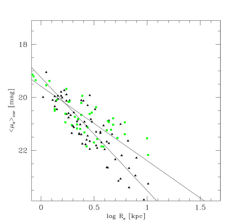
Figure 4: The bisector fits for the JFK sample of early-type galaxies in Coma subdivided into the morphological classes of ellipticals (squares) and S0s (triangles).

Table 3: Local comparison samples. The second column gives the number of galaxies of the respective sample, $a$ and $b$ are the zeropoints and slopes of the bisector fit to the respective $B$ band Kormendy relations. The values in brackets are $a$ and $b$ of the least-square fits.

sample	nog	a	b
Coma JFK: all ($12.14\leq B\leq 16.76$)	147	19.46 (19.79;18.91)	3.46 (2.73;4.63)
Coma JFK: $B<16.2$	108	19.17 (19.51;18.65)	3.59 (2.94;4.56)
Coma JFK: “HST” FOV	74	19.50 (19.81;19.00)	3.45 (2.77;4.53)
Coma JFK: all with $\sigma$ ($12.14\leq B\leq 16.75$)	92	19.60 (19.82;19.27)	2.72 (2.24;3.43)
Coma JFK: $\sigma>140$ ($12.14\leq B\leq 16.75$)	62	19.44 (19.59;19.27)	2.64 (2.35;3.01)
Coma JFK: $\sigma>200$ ($12.14\leq B\leq 16.75$)	24	19.32 (19.40;19.24)	2.43 (2.30;2.58)
Coma JFK: $\sigma>250$ ($12.14\leq B\leq 16.75$)	7	19.49 (19.54;19.45)	2.18 (2.13;2.24)
Coma JFK: $B<16.5$ ($68\leq\sigma\leq 386$)	85	19.51 (19.73;19.20)	2.81 (2.35;3.45)
Coma JFK: $B<16.0$ ($81\leq\sigma\leq 386$	64	19.30 (19.57;18.91)	2.96 (2.47;3.64)
Coma JFK: E only	44	19.58 (19.83;19.18)	2.81 (2.22;3.76)
Coma JFK: S0/SB0 only	78	19.25 (19.53;18.87)	4.27 (3.66;5.10)
Coma JFK: S0 with $\mathrm{\langle\-\mu_{e}\rangle_{cor}}<22$	65	19.44 (19.78;18.83)	3.68 (2.81;5.23)
Coma JFK: E with $\log R_{e}<1$kpc	42	19.52 (19.79;19.06)	3.02 (2.33;4.20)
Coma SBD: all	39	19.80 (19.88;19.72)	2.18 (2.03;2.35)
Coma SBD: no cDs	36	19.75 (19.91;19.53)	2.33 (1.94;2.89)
Coma SBD: E only	25	19.70 (19.76;19.62)	2.23 (2.11;2.37)
Coma SBD: S0/SB0 only	14	19.86 (20.03;19.58)	2.42 (1.90;3.23)
Coma JFK: same as SBD	39	19.63 (19.77;19.45)	2.46 (2.17;2.82)

As a second example we take the data of Saglia et al. (Saglia et al., 1993, SBD), which we re-calibrated and analyzed in the same manner as we did with the distant galaxies Bender et al. (1998). This sample has the advantage that it ensures a uniform fitting procedure for both the local and distant galaxies. Despite of being morphologically selected, this sample comprises both E and S0/SB0 galaxies but being restricted to the central part of the cluster does not contain any post-starburst galaxy of Caldwell et al. Caldwell et al. (1993) and, therefore, is a fair comparison to the distant spectroscopically selected cluster samples. In Table 3, we report the fit parameters to the Kormendy relation derived for this sample, too. A slightly different slope is found when we either include or exclude the three brightest E galaxies. As with the JFK sample a larger slope is found for a subsample of only S0/SB0 galaxies than for one of only ellipticals, but the difference is marginal.

We conclude that the slope of the Kormendy relation for cluster galaxies is in the range $2.2...3.6$, with a tendency to increase from the earlier to the later galaxy types. In the following we will consider both the Coma JFK and SBD samples as the local reference to determine the evolution of the Kormendy relation. Thus, we are able to estimate how the incompleteness of the SBD sample effects the results.

4.2 The method

In order to derive the luminosity evolution of ET cluster galaxies one has to compare the surface brightnesses as given by the Kormendy relation of a distant cluster to a local one. Most authors have made this comparison by choosing one slope for the Kormendy relation for both distant and local clusters, and looking at the variation of the surface brightness at a fixed standard effective radius of $1\,\mathrm{kpc}$ (i.e. the variation of the zeropoint of the Kormendy relation at $\log R_{e}=0$). This corresponds to assuming that (i) the slope of the Kormendy relation is independent of redshift; (ii) that its dependence on the ET galaxies selection is negligible; (iii) that at fixed $R_{e}$ there is a one to one correspondence between galaxies in the local and distant clusters. There is no a priori reason for these three assumptions to be valid, and indeed we have shown in the previous section that in the Coma cluster there is a dependence of the slope on the galaxy morphological subclass (and on the velocity dispersion range).

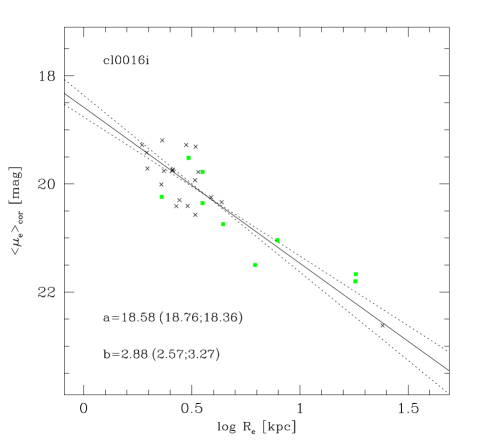
Figure 5: The Kormendy relation of cl0016i-galaxies. The solid line represents the bisector fit, the dotted lines are the lsq fits with variables interchanged. $a$ is the zeropoint, $b$ the slope of the bisector fit (values in brackets correspond to the lsq fits). The squares are galaxies with $d/b>0.2$.

In order to evaluate the evolution of the surface brightness of ET galaxies in clusters taking into account a possible variation of the slope of the Kormendy relation with redshift we proceed in two ways:

(1) fitting independently the Kormendy relations for the various high $z$ clusters and comparing them to the relation derived for Coma;

(2) imposing a fixed slope for the Kormendy relation in all the clusters, and exploring the derived luminosity evolution for a range of values for this slope.

4.3 The Kormendy relations in the distant clusters

Before we describe how the Kormendy relation depends on redshift, we first make sure that there exists a correlation between $\mathrm{\langle\-\mu_{e}\rangle_{cor}}$ and $\log\-R_{e}$ for the distant galaxy samples in a statistical sense. We performed a Spearman’s rank analysis and find that all samples with more than ten galaxies show indeed a correlation on the 99% probability level.

Figure 6: The (observed) Kormendy relation (dotted lines) for the distant cluster sample cl0016i (triangles) compared with the local sample (squares). The solid line represents the magnitude limit, which is shifted to the Coma SBD sample according to the calculated distance modulus and the expected luminosity evolution. The dashed line is the fit to this reduced sample.

For each distant cluster we determine the slope and zero points of the Kormendy relations for all ET galaxies (i.e., no E$+$A) by performing a bisector fit, as done for the Coma cluster. The results for each cluster are listed in Table 4. Fig. 5 shows the fit for cl0016i as an example. The slopes of the Kormendy relations for the distant clusters scatter between 2.2 and 3.5, which is within the range of the quoted local slopes (see Table 3). This indicates that the slope of the Kormendy relation does not change significantly with redshift. Since the effective radii of the galaxies in the distant clusters span a similar and wide range ($2.5\la\-R_{e}/\mathrm{kpc}\la 20$) (see Table 1), this implies that on the average the stellar populations of smaller ellipticals have not evolved from $z=0.6$ until today in a markedly different way with respect to those of larger ellipticals. A natural explanation for this is that the mean ages of the stars in small galaxies are not very different from those in large galaxies, implying a rather old age and high formation redshifts for their stellar populations, independent of the size of the early-type galaxies.

The differences in the zeropoints $a$ in Table 4 with respect to the same value for Coma reflect the surface brightness evolution of galaxies with $R_{e}=1$kpc, having adopted the Kormendy relation which best fits the data for the individual clusters. It can be noticed that for the four clusters at $z\approx 0.4$ we find a substantial scatter of these zeropoints. This stems from having considered the zeropoint at $R_{e}=1$ kpc. To describe the global evolution of cluster ellipticals, it is more meaningful to compare the surface brightnesses at the median value of the effective radii distribution ($\langle\log R_{e}\rangle$). Indeed the scatter of the surface brightness at $\langle\log R_{e}\rangle$ for the 4 clusters at $z\approx 0.4$ is substantially reduced (see column 6 of Table 4).

Figure 7: The distribution of the residual surface brightnesses $\Delta\mathrm{\mu}_{i}$ of cl0016i (triangles) and Coma SBD (squares) around their median value (solid line). The $\Delta\mathrm{\mu}_{i}$ of cl0016i were calculated here with the slope $b$ fixed to the Coma SBD value of $2.18$ instead of $2.88$ of the free bisector fit and are shown already reduced by the evolution $\Delta M_{\mathrm{fixed}}$.

Selection effects must be taken into account before these values can be used to derive the luminosity evolution. Obviously for the Coma cluster the distribution of effective radii extends down to much lower values than those reached in the distant samples. In order to apply similar selections for both the distant and the local samples, we cut off the Coma samples at a suitable magnitude limit. In this way we also minimize to first order the bias induced by the galaxy distribution in $\sigma$ (see Fig. 3). To determine the magnitude cut-off in the distant clusters introduced by the selection of the ET galaxies we go back to Eqs. (4) and (5). The maximum of the total magnitudes of all galaxies $i$ in a given sample represents the respective magnitude limit:

$$B_{\mathrm{lim}}=\max_{i}\left(\mathrm{\langle\mu_{e}\rangle}_{B,i}-5\log(r_{e,i})-2.5\log(2\pi)\right)$$ (8)

This limit is then applied to the Coma sample taking into account the difference in distance modulus. This procedure may not be correct, due to the luminosity evolution of individual galaxies. For example, passive evolution will force the fainter galaxies in the distant clusters to fade below the magnitude limit determined the way just described. To correct for this, we have to assume a luminosity evolution for the galaxies at the faint end of the distribution, $\Delta M_{B,\mathrm{lim}}$. As a first attempt we take a fading of $\Delta M_{B,\mathrm{lim}}=0.5$ and $0.66$ $\mathrm{mag}$ for the clusters at $z=0.4$ and $0.55$, respectively. These values are close to what is expected from Bruzual and Charlot models for the passive evolution of old stellar populations, and in the following will be referred to as initial set of parameters. Different values for the $\Delta M_{B,\mathrm{lim}}$ are explored later. Fig. 6 illustrates how the magnitude cut-off is implemented to estimate the luminosity evolution for Cl 0016$+$16.

To summarize, for each image of each cluster we construct the median $R_{e}$, calculate the surface brightness at this median $R_{e}$ from the Kormendy relation found for the ET cluster members in the specific image, and compare it to the surface brightness coming from the Kormendy relation constructed for the subsample of Coma ET galaxies brighter than the appropriate cut-off magnitude, evaluated at $\langle\log R_{e}\rangle$. The results are listed in columns 6 to 8 of Table 4. The luminosity evolution determined with this free slope approach is referred to as $\Delta M_{\mathrm{free}}$.

The last columns in Table 4 list the estimate of the evolution of the surface brightness with the second method, i.e. enforcing the same slope for the Kormendy relation in both the local and the distant clusters. We initially choose $b=2.18(3.46)$, which is appropriate for the Coma SBD (JFK) sample. The residual surface brightness of a galaxy $i$ in a specific image is defined as:

$$\Delta\mathrm{\mu}_{i}=\langle\mathrm{\mu}_{e}\rangle_{\mathrm{cor},i}-b\log R_{e,i}$$ (9)

The analogous value for Coma is derived considering only ET galaxies brighter than the appropriate cut-off. We prefer median values instead of means as a robust procedure to take care of outliers. The luminosity evolution determined with this approach is referred to as $\Delta M_{\mathrm{fixed}}$. Figure 7 describes the method for one cluster. Note that the residuals are not equally distributed around the fit: for this case, the actual slope of the Kormendy relation is $2.88$, while a fixed slope of $2.18$ has been adopted to compute the median surface brightness. Note that the difference between the two numbers is not significant in the light of Table 3.

Table 4: Results for the initial set of parameters (SFD extinction, $H_{0}=60\,\mathrm{km\,s^{-1}\,Mpc^{-1}},q_{0}=0.1$, $\Delta M_{B,\mathrm{lim}}=0.5(0.66)\mathrm{mag}$ at $z=0.4(0.55)$). Col. 3: number of galaxies used for the fits, Cols. 4. & 5.: zeropoint and slope of the bisector fit, Col. 6: surface brightness at the median effective radius of the sample calculated according to $a$ and $b$, Col. 7: the same for the Coma sample (SBD or JFK) which was reduced by the relevant magnitude cut-off, Col. 8: difference between $\mu(\langle R_{e}\rangle)$ and $\mu(\langle R_{e}\rangle)_{c}$. Col. 9: median value of the residual surface brightnesses $\Delta\mathrm{\mu}_{i}$, Col. 10: the same for the reduced Coma sample, Col. 11: difference between $\langle\Delta\mu\rangle$ and $\langle\Delta\mu_{c}\rangle$. Cluster samples written in italic are not used in the statistical analysis because they contain too low a number of galaxies ($<10$).

cluster	z	nog	a	b	$\mu(\langle R_{e}\rangle)$	$\mu(\langle R_{e}\rangle)_{c}$	$\Delta M_{\mathrm{free}}$	$\langle\Delta\mathrm{\mu}\rangle$	$\langle\Delta\mathrm{\mu_{c}}\rangle$	$\Delta\-M_{\mathrm{fixed}}$
ComaSBD	0.024	39	19.80	2.18	20.69	20.67	0.02	19.75	19.75	0.00
a370v	0.375	9	17.40	4.52	20.25	20.93	$-$0.68	18.86	19.64	$-$0.77
a370r	0.375	17	18.71	2.52	20.39	21.02	$-$0.64	18.95	19.64	$-$0.69
a370i	0.375	9	18.14	3.81	20.26	20.78	$-$0.52	19.11	19.64	$-$0.53
cl1447r	0.389	31	18.77	3.51	20.24	20.70	$-$0.46	19.30	19.75	$-$0.44
cl0939v	0.407	8	19.18	2.70	20.59	20.88	$-$0.28	19.58	19.69	$-$0.12
cl0939r	0.407	26	19.34	2.58	20.43	20.73	$-$0.29	19.31	19.75	$-$0.44
cl0939i	0.407	6	19.92	1.27	20.53	20.80	$-$0.27	19.56	19.69	$-$0.13
cl0303r	0.416	24	19.06	2.88	20.58	20.86	$-$0.28	19.42	19.67	$-$0.25
cl0016v	0.550	30	18.17	3.23	19.75	20.66	$-$0.91	18.75	19.64	$-$0.89
cl0016i	0.550	28	18.58	2.88	20.07	20.80	$-$0.73	18.96	19.65	$-$0.69
ComaJFK	0.024	147	19.46	3.46	20.97	20.97	0.01	20.04	20.04	0.00
a370v	0.375	9	17.40	4.52	20.25	20.89	$-$0.64	18.86	19.54	$-$0.67
a370r	0.375	17	18.71	2.52	20.39	21.20	$-$0.81	18.95	19.67	$-$0.72
a370i	0.375	9	18.14	3.81	20.26	20.81	$-$0.55	19.11	19.62	$-$0.51
cl1447r	0.389	31	18.77	3.51	20.24	20.82	$-$0.59	19.30	19.96	$-$0.66
cl0939v	0.407	8	19.18	2.70	20.59	21.07	$-$0.48	19.58	19.85	$-$0.28
cl0939r	0.407	26	19.34	2.58	20.43	20.92	$-$0.49	19.31	20.04	$-$0.72
cl0939i	0.407	6	19.92	1.27	20.53	20.94	$-$0.41	19.56	19.89	$-$0.33
cl0303r	0.416	24	19.06	2.88	20.58	21.03	$-$0.45	19.42	19.80	$-$0.38
cl0016v	0.550	30	18.17	3.23	19.75	20.60	$-$0.86	18.75	19.67	$-$0.92
cl0016i	0.550	28	18.58	2.88	20.07	20.88	$-$0.81	18.96	19.78	$-$0.81

Figure 8: Luminosity evolution derived from the Kormendy relations for the initial set of parameters (see text). Top panels: local reference sample: Coma SBD, bottom panels: local reference sample: Coma JFK. Left panels: free bisector fit method, right panels: fixed slope fit method (see text for explanations). Solid curves: expected evolution from a BC98 model with $z_{f}=4$ and IMF slope $x=2.35,1.35$ (Salpeter) and $0.35$ (top to bottom). The points for the V and I images of Cl 0016 are shifted in $z$ for better visibility. The errorbars are the quadratic sum of the mean $\sigma_{c}$ and the standard deviation of the Coma sample.

The results of the two methods are visualized in Fig. 8 for the images in which more than 10 galaxies could be used (i.e. the $R$ images of Abell 370, Cl 0303$+$17, Cl 0939$+$47 and Cl 1447$+$26, and the $V$ and $I$ images of Cl 0016$+$16) and compared to both Coma samples (SBD and JFK). The errors are computed in the following way: we first calculate the standard deviation of the residuals of all galaxies ($n_{g}$) around the bisector fit to the $\mathrm{\langle\mu_{e}\rangle_{cor}}$–$\log(R_{e})$ data for each cluster individually: $\sigma_{g}=\sqrt{\sum_{i=1}^{n_{g}}(x_{i}-\bar{x})^{2}/(n_{g}-1)}$ with $x=\mathrm{\langle\mu_{e}\rangle_{cor}}-b\cdot\log(R_{e})-a$ and $\bar{x}=\sum_{i=1}^{n_{g}}x_{i}/n_{g}$. The average observed scatter is then taken to be the combined standard deviation of all clusters ($n_{c}$): $\sigma_{a}=\sqrt{\sum_{i=1}^{n_{c}}\sigma_{g,i}^{2}/n_{c}}$. The error for each cluster is then: $\sigma_{c}=\sigma_{a}/\sqrt{n_{g}}$. Note that the scatter in the Kormendy relation arises mainly from neglecting the velocity dispersion of the tight Fundamental Plane and is little augmented by the measurement errors. See Sect. 6 for a discussion of the errors induced by the K-corrections.

The overall redshift evolution of the surface brightness of ET galaxies derived with the two methods and compared to the two local reference samples is quite similar. Distinctive differences between the same individual samples in the 4 panels of Fig. 8 are not significant given the large errors in the single data points. Because both our methods rely on median values the incompleteness of the Coma SBD sample does not have a systematic effect on the derived evolution. The overall slightly higher values of $\Delta M$ for the JFK sample are rather the result of the transformation from Gunn $r$ to Johnson $B$ magnitudes. The predictions of passive evolution models are also shown in Fig. 8. These are BC98 models calculated for a 1-Gyr-burst population of solar metallicity forming at $z=4$ ($t_{\mathrm{gal}}=12$ Gyr) and IMF slopes of $x=2.35,1.35$ (Salpeter) and $0.35$, respectively. The data points for the cluster samples are compatible with the considered models within the 1-$\sigma$-error in all four panels.

5 Effects of the assumptions

The luminosity evolution derived in the previous section using method (1) or (2) depends on various assumptions. In the following we explore the effects of the assumptions used for method (2):

(i) the value of the slope of the Kormendy relation adopted for all the clusters,

(ii) the value of the $\Delta M_{B,\mathrm{lim}}$ parameter,

(iii) the selection criteria for the early type galaxies in the various clusters.
Similar tests have been performed for method (1). The detected systematic effects are of similar size. In Fig. 9 to 14 the luminosity is labelled $\Delta M_{\mathrm{evol}}$.

As discussed before, the slope of the Kormendy relation depends on the range of the velocity dispersions, and on the morphological selection criteria. It is therefore appropriate to explore the effect on the luminosity evolution by adopting different slopes for the Kormendy relation in our clusters. We repeat the determination of $\Delta M_{\mathrm{fixed}}$ as in the previous section (with Coma SBD as the local sample), assuming $b=1.9,2.3,2.7,3.1$, and $3.5$, respectively. These values span the range of plausible slopes observed in local samples, see Table 3. The results are shown in Fig. 9, where the different symbols refer to the different slopes, and the line is the expected passive evolution computed for the BC98 1-Gyr-burst model (only Salpeter IMF). The values of the luminosity evolution obtained with these different slopes scatter around those obtained with the slope closest to the free bisector fit slope. The differences in the derived evolution arise from the fact that the distant galaxy samples are not fitted by their appropriate slope. This can be seen in the distribution of the residual surface brightnesses of cl0016i in Fig. 7.

Another important assumption made in the derivation of the luminosity evolution concerns the value of $\Delta M_{B,\mathrm{lim}}$ applied to the ET galaxies in Coma. It is worth mentioning that the application of a $\Delta M_{B,\mathrm{lim}}$ does not influence the distant galaxy samples at all. It only adds or subtracts some Coma ellipticals at the faint end of their magnitude distribution, thus affecting $\langle\Delta\mathrm{\mu_{c}}\rangle$, which is compared to the not changing median value of the distant samples. To test the influence of this parameter on the derived luminosity evolution we repeat the determination of $\Delta M_{\mathrm{fixed}}$ for two more values of the $\Delta M_{B,\mathrm{lim}}$ parameter. Assuming no evolution at all (i.e. $\Delta M_{B,\mathrm{lim}}=0$), the effect on the derived luminosity evolution is rather small, as can be seen in Fig. 10. On the other extreme side, we take twice the value expected from passive evolution models: $\Delta M_{B,\mathrm{lim}}=1.0$ $\mathrm{mag}$ for the clusters at $z=0.4$ and $\Delta M_{B,\mathrm{lim}}=1.32$ $\mathrm{mag}$ for Cl 0016$+$16 at $z=0.55$. The magnitude cut-off for Coma now implies that virtually the whole SBD sample is used for the comparison with the distant clusters. As a result, $\langle\Delta\mathrm{\mu_{c}}\rangle$ for the selected galaxies in Coma stays constant at a high level, and the derived evolution is increased with respect to the case discussed in the previous section. However, even with this extreme assumption about the luminosity evolution of the fainter galaxies, the derived surface brightness evolution is still within the 1-$\sigma_{c}$ error (see Fig. 10).

Finally, we study the influence of our galaxy selection criteria. Up to now, the considered samples comprised all galaxies whose spectral energy distributions resemble those of early-type galaxies, regardless of their morphology. To exclude any contribution to the integrated light by a young stellar population which might reside in a disk component we reduce our galaxy sample for each cluster now to those galaxies that have a disk-to-bulge ratio $d/b\leq 0.2$. These subsamples should contain neither lenticular (S0) galaxies nor extreme disky ellipticals. The original galaxy samples are reduced by about a factor of two by this selection (see Table 1). In spite of the appreciably lower number of objects, the newly determined values of the luminosity evolution are within the 1-$\sigma_{c}$ error with respect to those previously obtained for the galaxy samples including all early-type galaxies. In Fig. 11 we also show the results for the subsamples selected by $d/b>0.2$. It can be seen that there is no trend towards weaker or stronger evolution. This means that the original samples are not contaminated by galaxies with a disk population substantially younger than the global average. If the galaxies with high $d/b$-ratios in the distant clusters are really comparable to those classified as lenticular in the nearby Universe, then, there exists a number of S0 galaxies in clusters even at intermediate redshifts that have disks of mainly old stars. This is consistent with the local Fundamental Plane relation that shows no offset between E and S0 galaxies Jørgensen et al. (1996).

The values of the derived luminosity evolution does not change significantly, too, if we add a few E$+$A galaxies to the original sample of early-type galaxies (see Fig. 11). The fraction of E$+$As makes up about 10 to 20% of the resulting samples (Table 1). This could represent a lower limit to the global fraction of E$+$A galaxies, because we look at the cores of clusters, where E$+$As may be less frequent than in the outer parts (Belloni and Röser, 1996; Belloni et al., 1997b, and references therein). Most of the (spectroscopically classified) E$+$As have high $d/b$-ratios. This points to spiral galaxies as the progenitors of E$+$As and not ellipticals having had a small starburst Wirth et al. (1994); Belloni et al. (1997a); Wirth (1997). Nevertheless, the contamination of a sample of early-type galaxies by a small fraction of E$+$As does not change the Kormendy relation and the observed scatter is only slightly increased.

Figure 9: Luminosity evolution derived from the Kormendy relations assuming different slopes: filled triangle: $b=1.9$, filled square: $2.3$, filled circle: $2.7$, open triangle: $3.1$, open square: $3.5$. The errorbar in the lower left corner represents the quadratic sum of the mean $\sigma_{c}$ and the standard deviation of the Coma sample. The solid curve is the BC98 model with $z_{f}=4$ and Salpeter IMF.

Figure 10: Luminosity evolution derived from the Kormendy relations assuming different evolution a priori to find the magnitude cut-off for the Coma sample: circles: $\Delta M_{B,lim}=0$, squares: $\Delta M_{B,lim}$ according to our 1 Gyr burst passive evolution model, triangles: $\Delta M_{B,lim}$ twice as high.

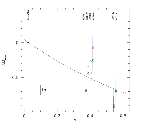
Figure 11: Luminosity evolution derived from the Kormendy relations for samples with different galaxy types: squares: original samples of Es, S0s and Sas, triangles: “no S0/Sas” (only galaxies with $d/b\leq 0.2$), crosses: “only S0/Sas” (only galaxies with $d/b>0.2$), circles: original samples with a few E$+$As added.

6 Modelling the luminosity evolution

We now investigate which evolutionary stellar population models can fit the data within their errors. For the comparison between models and observations we arbitrarily choose one specific set of data points, but take into account the systematic errors arising from this particular choice. We choose the luminosity evolution as given by $\Delta M_{\mathrm{fixed}}$ with respect to the Coma SBD sample, because having no post-starburst galaxies its selection is closest to the one applied for the distant clusters. We consider the derivation of $\Delta M_{\mathrm{fixed}}$ for our initial set of parameters with one exception: instead of applying the SFD absorptions we take the mean of SFD and BH values and, therefore, introduce another systematic error in our error budget. This error budget is summarized in Table 5. It comprises the average statistical error for a distant sample, $\sigma_{\mathrm{stat}}$, which is the quadratic sum of the mean $\sigma_{c}$ and the standard deviation of the Coma sample: $\sigma_{\mathrm{stat}}=\sqrt{\langle\sigma_{c}\rangle^{2}+\sigma_{\mathrm{Coma}}^{2}}\approx 0.14\,\mathrm{mag}$ and several systematic errors, which must be added linearly. There are three errors arising from the calibration of the magnitudes (see Sect. 3): determination of the zeropoint and color transformation, $\sigma_{\mathrm{zp}}\approx 0.07\,\mathrm{mag}$, K-correction, $\sigma_{\mathrm{kc}}\approx 0.04\,\mathrm{mag}$ (for the $R$ images of the $z=0.4$ clusters considered here, see Table 2), and extinction, $\sigma_{\mathrm{ex}}\approx 0.03\,\mathrm{mag}$ (half the average difference between SFD and BH values). Another systematic error is introduced by the selection of a given fixed slope for the Kormendy relation for all clusters. From the distribution of the derived values of $\Delta M_{\mathrm{fixed}}$ for different slopes $b$ we estimate this error to be $\sigma_{\mathrm{fs}}\approx 0.04\,\mathrm{mag}$ (see Section 5). Therefore, the systematic errors add up to even a higher value than the average statistical error (see Table 5).

Table 5: Errors introduced in the derivation of the luminosity evolution arising from the observed scatter, the determination of zeropoint, K-correction and extinction, and the choice of a given fixed slope.

$\sigma_{\mathrm{stat}}$	$\sigma_{\mathrm{zp}}$	$\sigma_{\mathrm{kc}}$	$\sigma_{\mathrm{ex}}$	$\sigma_{\mathrm{fs}}$	$\sigma_{\mathrm{syst}}$	$\sigma_{\mathrm{tot}}$
0.14	0.07	0.04	0.03	0.04	0.18	0.32

The total error is quite large, as it amounts already to half the expected value of the luminosity evolution in passive evolution models at $z=0.4$ (see below). Seen together with the scatter of the data points of different clusters at the same redshift it is obvious that there is not a single evolutionary model favoured but a broad range of models can fit the data. In the following we explore the different allowed star formation histories using BC98 models.

If we first confine to pure passive evolution models with an initial 1-Gyr star burst, it can be seen in Fig. 12 (solid lines) that the formation epoch could be at any redshift larger than $\approx 2$, corresponding to epochs greater than $\approx 10$ Gyrs ago. A more recent formation would yield a too large luminosity evolution. On the other hand our measured evolution reflects the behaviour of the average properties of ET galaxies in the clusters. Individual galaxies could well lie away from the average relation without violating our previous finding that the slope of the Kormendy relation does not change significantly with $z$ given the large uncertainties in the local slope (see Section 4.3). Therefore, differences in the formation redshift between individual galaxies and the majority of the whole cluster sample are possible even within the framework of passive evolution. The dashed lines in Fig. 12 show the effect on the average Kormendy relation of assuming that some fraction of the ET galaxies in the clusters formed at lower redshifts. It can be seen that if we assume that 10% of the observed galaxies had formed only at $z_{f}=1$ (with the remaining 90% at $z_{f}=4$), and both subsamples were equally distributed in $R_{e}$, the effect on the average Kormendy relation would be small. Only the case of 50% galaxies formed at $z_{f}$=4 and 50% galaxies at 1 is highly disfavoured, when considering the highest redshift cluster.

Figure 12: Passive evolution 1-Gyr-burst models with formation epochs $z_{f}=1,2,4$ and $11$ (Salpeter IMF) superposed as solid lines onto the observed data with their statistical (solid errorbars) and systematic errors (dashed errorbars). Dashed lines are 1:1, 1:4 and 1:10 combinations (bottom to top) between $z_{f}=1$ and $z_{f}=4$ models (see text).

In the same way, models different from a pure burst are also compatible with the data. Here, we investigate BC98 $\tau$-models which have exponentially decreasing star formation rates. As an example we show in Fig. 13 the predictions from models with timescales $\tau=2/3,1$ and $2\mathrm{Gyrs}$, all for a formation redshift $z_{f}=4$ and Salpeter IMF. The dashed and dotted lines are the BC98 models for an instantaneous burst and a 1-Gyr burst, and are shown for comparison. Our spectrophotometric classification (see Sect. 2) assigns model galaxies with $\tau<2$ to the family of early-type galaxies. The $\tau$ model with star formation timescales shorter than 1 Gyr still gives a nice representation of the data. Thus models with currently ongoing star formation on a low level can not be strictly ruled out, although most of the stars in the ET galaxies must have formed at large redshift. The value of the limit on $\tau$ depends on the assumed IMF exponent, and longer star formation timescales would be allowed in combination with steeper IMF slopes. However, other arguments tend to disfavour IMF slopes steeper than Salpeter in ET galaxies (Arimoto & Yoshii 1987, Matteucci 1994, Thomas, Greggio & Bender 1999).

Figure 13: Different evolutionary BC98 models with formation epoch $z_{f}=4$ superposed as lines onto the observed data with their statistical (solid errorbars) and systematic errors (dashed errorbars). From top to bottom: SSP, 1-Gyr burst, $\tau=2/3,1$ and $2$ models.

As a final example, we consider a scenario where an elliptical galaxy experiences a sudden addition of a small second stellar population on top of the old main component. A possible realization would be the accretion of a small gas-rich galaxy leading to a second short burst of star formation. We have already seen that the contamination of a sample of early-type galaxies by a few E$+$As would not change dramatically the Kormendy relation itself. Our E$+$A templates comprised models with a second burst lasting 0.25 Gyrs, amounting to an additional 20% of the mass of the underlying old population. A galaxy with a less prominent second burst could easily be hidden in our ET samples. The presence of the second burst could be revealed by our spectrophotometric identification if it occurred less than 2 Gyrs before $z_{\mathrm{obs}}$. If it happened earlier, the E$+$As signatures would not have been detected by our method. From the numerous possible model realizations of such an event we pick up an example which lies close to our detection limit of a second burst: we choose a model galaxy that had an initial 1-Gyr burst of star formation lasting from $z=4$ until $z=2.6$ and that gets an additional 10% of mass in a second 0.2-Gyr burst at $z=0.63$, corresponding to 2 Gyrs before $z=0.4$ in our cosmology. Fig. 14 shows that the difference in the luminosity evolution at $z=0.4$ between this particular model and a pure burst model corresponds to about 1 $\sigma_{c}$ error. We also plot the model evolution for samples having different mixtures of these kind of galaxies and single burst passively evolving galaxies which reduces the difference from the pure burst model even further.

Figure 14: Evolutionary BC98 model representing an elliptical galaxy that has experienced a second burst at $z=0.63$ as specified in the text (dot-dashed line) compared to the single 1-Gyr burst model (solid line). Dashed lines are 1:1, 1:4 and 1:10 combinations between the two models.

7 Summary and conclusions

We have investigated samples of elliptical galaxies in four clusters at redshifts around $z=0.4$ and one at $z=0.55$. The cluster member galaxies were selected by spectral type from our ground-based spectrophotometric observations that allowed the classification of the galaxies as ellipticals, spirals, irregulars and E$+$As by comparing the low-resolution SEDs with template spectra. The structural parameters were determined from HST images by a two-component fitting of the surface brightness profiles. With this method we derived not only accurate values of the total magnitude and the effective radius of a galaxy down to $B_{\mathrm{tot}}=23$ $\mathrm{mag}$, but could also detect a disk component if present down to the resolution limit and derive disk-to-bulge values.

We constructed the rest-frame $B$-band Kormendy relations ($\mathrm{\langle\-\mu_{e}\rangle_{cor}}-\log(R_{e})$) for the various samples and find no significant change of the slope with redshift. Because all the samples span a similar range in $\log(R_{e})$, this indicates that on average the stellar populations of smaller ellipticals do not evolve in a dramatically different manner than larger ones at $z<0.6$ implying a high redshift of formation for the majority of the stars in early-type cluster galaxies irrespective of the galaxies’ size. The residuals of the Kormendy relations have a rather high dispersion ($\sigma_{\mathrm{stat}}=0.14$ $\mathrm{mag}$), which is mainly due to having neglected the third parameter (the velocity dispersion of the Fundamental Plane) and are little augmented by measurement errors. The systematic errors arising from the calibration of the HST magnitudes to rest-frame $B$ magnitudes (zeropoint and color transformation, K-correction, and reddening) amount to the same value.

We have shown that the actual values of the derived luminosity evolution depends on a number of different assumptions starting with the choice of the local comparison sample. A further assumption to be made is the appropriate magnitude cut-off for the local sample, which must be restricted to the magnitude distribution of the respective distant cluster in order to have an unbiased comparison. For our Coma SBD sample we found that the variation of this cut-off by half a magnitude results in differences of about $0.05\,\mathrm{mag}$ in the estimated luminosity evolution of a distant cluster sample. As mentioned in the Introduction, most authors using the Kormendy relation take a fixed slope $b$ when fitting the data of different clusters. We find that the derived luminosity evolution remains the same within about $0.04\,\mathrm{mag}$ when the value of the fixed slope is varied within the range found for local galaxy samples.

Compared to our Coma SBD early-type galaxies we find for our initial set of parameters an average brightening of $\Delta B=-0.42$ $\mathrm{mag}$ at $z=0.4$ and $\Delta\-B=-0.73$ $\mathrm{mag}$ at $z=0.55$. The scatter between the four clusters at $z=0.4$ ($\sigma=0.15$ $\mathrm{mag}$) is close to the statistical error for the individual data point. Given the dependence of the derived brightening on the various assumptions it is not surprising that other studies find different values for the same clusters, especially when taking into account that already the calibration of the HST images are performed using other values for the zeropoint, K-correction, and extinction. For example, Schade et al. Schade et al. (1996) give $\Delta\-B=-0.22\pm 0.19$ $\mathrm{mag}$ for a sample of 6 galaxies in the $I$ frame of Abell 370 and $\Delta\-B=-0.57\pm 0.13$ $\mathrm{mag}$ for 28 ellipticals in the $I$ frame of Cl 0016$+$16 assuming a fixed slope $b=3.33$. Barger et al. Barger et al. (1998) get $\Delta B=-0.45\pm 0.09$ $\mathrm{mag}$ (judging from their Figure 5b) for three clusters at $z=0.4$ and $\Delta\-B=-0.62\pm 0.1$ $\mathrm{mag}$ for three clusters at $z=0.55$ assuming a fixed slope $b=3.0$ and no colour dependence of the HST zeropoints.

Contrary to previous studies, we could reliably detect the post-starburst nature of a galaxy from our spectrophotometry and exclude these galaxies from the samples of early-type galaxies. If we contaminate these samples by the few E$+$A galaxies found in the core of the clusters (about 10% of the whole sample) we still do not find any excess brightening of the Kormendy relations but only variations within the 1 $\sigma_{c}$ error. This is in accordance with model expectations by Barger et al. Barger et al. (1996) who find only a small average brightening of the spheroidal galaxy population of clusters at $z=0.3$ by the inclusion of E$+$A galaxies.

There is also no systematic trend towards stronger or weaker evolution when we subdivide the samples into early-type galaxies having larger or lower disk-to-bulge values than $d/b=0.2$. This indicates that most of the (spectroscopically selected) galaxies with prominent disks in the cores of distant clusters have disk populations consisting still mainly of old stars. There is no significant contribution to the light by young stars as would be expected if those galaxies were the recent remnants of spiral galaxies that lost their gas due to some cluster influence.

The presented luminosity evolution of early-type galaxies since intermediate redshifts as derived here from the Kormendy relations is compatible with passive evolution models. But given the relatively large total error (not always considered in the past), the models are not constrained very much. All burst models with formation redshift $z_{f}>2$ can reasonably fit the data. Models with an exponentially decreasing star formation rate are also adequate, as long as the e-folding timescale $\tau$ is less than 2. We have shown that galaxies with a younger formation epoch or a weak second burst of star formation could be easily hidden in the Kormendy relation.

All in all, it is evident that the comparison of the Kormendy relations at various redshifts does not constrain the luminosity evolution of cluster ellipticals strongly enough to be able to decide whether pure passive evolutionary models or models with exponentially decaying star formation (which would fit better to hierarchical galaxy formation) can better match the data at redshifts up to $z=0.6$. The significance of this method would be increased if more observations of clusters at many other (and higher) redshifts were combined although the internal scatter per cluster would not be decreased. For few clusters, the investigation of the evolution of the tight Fundamental Plane in connection with the Mg-$\sigma$ relationship gives more accurate and constraining results.

Appendix A Photometric parameters of the distant galaxy samples

In this appendix we present the photometric parameters for all the investigated galaxies, not only the early-type galaxies, which are members of the distant clusters of this study. The parameters were derived by the method described and extensively tested by Saglia et al. Saglia et al. (1997), which applies a PSF broadened 2-component ($r^{1/4}$ and exponential) fitting procedure. There is a separate table for each cluster sample of Table 1.

Explanation of the table columns:
Col. 1 (galaxy): Identification number of the galaxy. For clusters Cl 0939$+$47 and Cl 0016$+$16, they correspond to the ID number of Belloni and Röser Belloni and Röser (1996). For Abell 370, they correspond to the ID number of Soucail et al. Soucail et al. (1988). For clusters Cl 1447$+$26 and Cl 0303$+$17 (and Abell 370), galaxy identifications of Smail et al. (Smail et al., 1997, S97) are given, too.
Col. 2 (type): The numbers correspond to the SED model which best fits the spectrophotometric data of the galaxy as described in Belloni et al. Belloni et al. (1995): $1=$ early-type (E, S0, or Sa), $2=$ spiral (Sbc), $3=$ spiral (Scd), $4=$ irregular (Im), $5-10=$ post-starburst (E$+$A) model.
Col. 3 ($r_{e}$): Global effective radius in arcsec.
Col. 4 ($\log R_{e}$): Global effective radius in kpc for $H_{0}=60\,\mathrm{km\,s^{-1}\,Mpc^{-1}},q_{0}=0.1$.
Col. 5 ($M_{\mathrm{t}ot}$): Total magnitude transformed to the respective Johnson–Cousin magnitude and corrected for galactic extinction according to SFD ($M_{\mathrm{t}ot}=M_{\mathrm{i}nst}+{\mathrm{Z}P}+A$). See Table 2 for the values of ZP and $A$(SFD) for the different cluster samples.
Col. 6 ($B_{\mathrm{r}est}$): Total magnitude transformed to restframe Johnson $B$ ($B_{\mathrm{r}est}=M_{\mathrm{t}ot}-K$). See Table 2 for the values of $K$ for the different cluster samples.
Col. 7 ($\langle\mu_{e}\rangle_{\mathrm{c}or}$): Effective mean surface brightness within $r_{e}$ in $B$ and corrected for the cosmological surface brightness dimming (see equation 6).
Col. 8 ($d/b$): Disk-to-bulge ratio ($F_{\mathrm{d}isk}/F_{\mathrm{b}ulge}$).
Col. 9 ($r_{e,b}$): Effective radius of the bulge component in arcsec.
Col. 10 ($h$): Disk scale length in arcsec.

Table 6: Photometric parameters for a370i

galaxy	S97	type	$r_{e}$	$\log R_{e}$	$M_{\mathrm{t}ot}$	$B_{\mathrm{r}est}$	$\langle\mu_{e}\rangle_{\mathrm{c}or}$	$d/b$	$r_{e,b}$	$h$
38	514	1	0.51	0.45	18.87	20.75	19.90	0.00	0.51	0.00
46	373	2	0.85	0.68	18.74	20.62	20.87	2.44	0.34	0.62
47	487	1	1.36	0.88	18.23	20.11	21.38	0.22	1.00	2.46
49	377	1	1.40	0.89	18.22	20.10	21.44	0.22	1.06	2.02
59	480	2	1.35	0.88	17.88	19.76	21.03	1.19	0.89	0.98
72	509	2	0.69	0.58	19.57	21.45	21.24	1.38	0.53	0.45
-	232	1	0.64	0.56	18.56	20.43	20.09	0.52	0.50	0.50
-	230	1	0.55	0.49	18.41	20.28	19.60	0.00	0.55	0.00
-	237	1	1.21	0.83	18.70	20.58	21.61	0.00	1.21	0.00
-	182	1	1.05	0.77	18.07	19.95	20.68	0.00	1.05	0.00
-	231	1	0.48	0.43	19.14	21.02	20.05	0.00	0.48	0.00
-	289	1	0.57	0.51	19.41	21.29	20.70	0.00	0.57	0.00

Table 7: Photometric parameters for a370r

galaxy	type	$r_{e}$	$\log R_{e}$	$M_{\mathrm{t}ot}$	$B_{\mathrm{r}est}$	$\langle\mu_{e}\rangle_{\mathrm{c}or}$	$d/b$	$r_{e,b}$	$h$
7	1	0.42	0.37	20.21	21.23	19.95	0.00	0.42	0.00
9	6	4.95	1.44	18.82	19.84	23.92	1.42	3.09	3.54
13	1	0.83	0.67	18.88	19.90	20.11	0.00	0.83	0.00
16	1	0.88	0.69	19.04	20.06	20.40	0.51	2.18	0.19
17	1	1.21	0.83	18.69	19.71	20.73	0.49	0.68	1.63
18	1	0.88	0.69	19.04	20.06	20.40	0.35	0.56	1.33
20	1	7.63	1.63	16.59	17.61	22.63	2.81	1.99	5.80
23	1	1.39	0.89	18.48	19.50	20.83	0.37	0.89	1.86
27	1	0.52	0.47	19.51	20.53	19.73	0.00	0.52	0.00
28	1	1.53	0.93	18.45	19.47	21.00	0.16	1.89	0.44
31	1	0.78	0.64	19.28	20.30	20.37	0.66	0.32	1.18
32	1	1.89	1.02	18.27	19.29	21.29	0.55	0.96	2.67
35	1	9.13	1.71	16.73	17.75	23.16	0.07	10.36	0.76
36	1	0.46	0.41	19.83	20.85	19.77	0.00	0.46	0.00
56	1	0.44	0.39	19.40	20.42	19.23	0.15	0.35	0.74
64	1	0.47	0.41	20.07	21.09	20.04	0.00	0.47	0.00
70	6	0.46	0.41	20.15	21.17	20.10	$\infty$	0.00	0.28
76	1	0.75	0.63	19.67	20.69	20.69	0.00	0.75	0.00
83	1	0.38	0.33	20.13	21.15	19.67	0.36	0.47	0.17

Table 8: Photometric parameters for a370v

galaxy	S97	type	$r_{e}$	$\log R_{e}$	$M_{\mathrm{t}ot}$	$B_{\mathrm{r}est}$	$\langle\mu_{e}\rangle_{\mathrm{c}or}$	$d/b$	$r_{e,b}$	$h$
38	514	1	0.56	0.49	20.68	20.43	19.78	0.00	0.56	0.00
46	373	2	0.85	0.68	20.43	20.18	20.43	3.25	0.28	0.60
47	487	1	1.49	0.92	19.97	19.72	21.20	0.08	1.72	0.11
49	377	1	1.13	0.80	20.33	20.08	20.95	0.00	1.13	0.00
59	480	2	1.31	0.86	19.71	19.46	20.65	3.06	0.50	0.92
72	509	2	0.61	0.53	20.73	20.48	20.01	2.75	0.24	0.43
-	232	1	0.63	0.54	20.57	20.32	19.92	0.96	0.38	0.50
-	230	1	0.57	0.50	19.90	19.65	19.04	0.00	0.57	0.00
-	237	1	1.19	0.82	20.57	20.32	21.32	0.00	1.19	0.00
-	182	1	0.97	0.73	19.97	19.72	20.26	0.00	0.97	0.00
-	231	1	0.50	0.44	20.98	20.73	19.83	0.00	0.50	0.00
-	289	1	0.76	0.63	21.12	20.87	20.90	0.17	1.04	0.10

Table 9: Photometric parameters for cl0016i

galaxy	type	$r_{e}$	$\log R_{e}$	$M_{\mathrm{t}ot}$	$B_{\mathrm{r}est}$	$\langle\mu_{e}\rangle_{\mathrm{c}or}$	$d/b$	$r_{e,b}$	$h$
40	1	0.38	0.41	20.14	21.76	19.73	0.18	0.49	0.10
43	4	0.26	0.25	21.07	22.69	19.85	$\infty$	0.00	0.6
48	1	0.91	0.79	20.00	21.62	21.50	0.39	0.91	0.54
51	1	0.29	0.29	20.43	22.05	19.42	0.00	0.29	0.00
56	1	0.34	0.37	20.37	21.99	19.76	0.00	0.34	0.00
70	1	0.33	0.36	20.90	22.52	20.24	0.60	0.33	0.20
73	7	0.41	0.44	20.10	21.72	19.85	1.11	0.10	0.51
95	1	0.41	0.44	20.55	22.17	20.30	0.00	0.41	0.00
97	1	0.64	0.64	19.99	21.61	20.74	0.55	0.71	0.35
122	1	0.48	0.52	19.19	20.81	19.31	0.00	0.48	0.00
126	1	0.34	0.36	19.84	21.46	19.19	0.00	0.34	0.00
133	1	0.52	0.55	20.07	21.69	20.35	0.54	0.24	0.89
139	1	3.52	1.38	18.18	19.80	22.62	0.12	4.29	0.64
141	3	0.77	0.72	19.42	21.04	20.58	0.32	1.29	0.19
150	1	2.63	1.26	17.99	19.61	21.80	0.37	2.19	2.07
152	1	2.64	1.26	17.85	19.47	21.67	0.29	3.55	0.93
156	1	0.52	0.55	19.49	21.11	19.78	0.33	0.36	0.62
160	1	0.64	0.64	19.61	21.23	20.34	0.00	0.64	0.00
164	1	0.44	0.47	19.37	20.99	19.28	0.00	0.44	0.00
175	1	0.33	0.36	20.68	22.30	20.01	0.00	0.33	0.00
176	1	0.39	0.43	20.73	22.35	20.41	0.00	0.39	0.00
179	1	0.50	0.53	19.59	21.21	19.78	0.00	0.50	0.00
180	1	0.38	0.41	20.16	21.78	19.75	0.00	0.38	0.00
181	1	0.45	0.48	19.56	21.18	19.52	0.25	0.33	0.59
185	1	1.15	0.90	19.03	20.65	21.04	0.87	0.50	1.23
187	1	0.57	0.59	19.77	21.39	20.25	0.00	0.57	0.00
188	1	0.27	0.27	20.39	22.01	19.28	0.00	0.27	0.00
191	1	0.44	0.48	20.47	22.09	20.41	0.00	0.44	0.00
193	1	0.48	0.51	19.82	21.44	19.93	0.00	0.48	0.00
207	7	0.30	0.31	20.20	21.82	19.28	0.44	0.14	0.88
215	1	0.29	0.29	20.71	22.33	19.72	0.00	0.29	0.00
222	1	0.48	0.52	20.46	22.08	20.57	0.00	0.48	0.00
234	7	0.39	0.43	20.44	22.06	20.13	0.00	0.39	0.00

Table 10: Photometric parameters for cl0016v

galaxy	type	$r_{e}$	$\log R_{e}$	$M_{\mathrm{t}ot}$	$B_{\mathrm{r}est}$	$\langle\mu_{e}\rangle_{\mathrm{c}or}$	$d/b$	$r_{e,b}$	$h$
40	1	0.41	0.45	22.47	21.54	19.71	0.00	0.41	0.00
48	1	1.35	0.97	21.86	20.93	21.67	1.72	0.62	1.03
51	1	0.38	0.42	22.35	21.42	19.42	0.00	0.38	0.00
56	1	0.33	0.36	22.69	21.76	19.47	0.00	0.33	0.00
68	1	0.42	0.45	21.24	20.31	18.50	0.00	0.42	0.00
70	1	0.84	0.76	22.54	21.61	21.32	0.00	0.84	0.00
73	7	0.47	0.50	22.14	21.21	19.64	0.98	0.16	0.54
84	7	0.61	0.62	22.20	21.27	20.30	2.28	0.18	0.48
86	7	0.32	0.34	23.11	22.18	19.81	0.55	0.65	0.10
87	1	0.28	0.28	22.88	21.95	19.28	0.00	0.28	0.00
92	7	0.45	0.48	22.44	21.51	19.84	0.63	0.90	0.15
95	1	0.49	0.52	22.72	21.79	20.31	0.00	0.49	0.00
97	1	0.69	0.68	22.29	21.36	20.66	0.47	0.92	0.30
109	7	0.65	0.65	21.77	20.84	19.98	0.44	0.55	0.48
112	7	1.19	0.91	20.78	19.85	20.31	$\infty$	0.00	0.71
126	1	0.32	0.35	22.25	21.32	18.96	0.00	0.32	0.00
139	1	3.64	1.40	20.58	19.65	22.55	0.11	4.38	0.60
144	1	0.34	0.37	23.09	22.16	19.94	0.00	0.34	0.00
146	1	0.27	0.27	22.97	22.04	19.29	0.95	0.71	0.10
150	1	1.70	1.06	20.28	19.35	20.59	3.85	0.18	1.28
152	1	1.97	1.13	20.64	19.71	21.27	0.34	2.87	0.66
156	1	0.52	0.55	21.85	20.92	19.60	0.00	0.52	0.00
160	1	0.71	0.69	21.90	20.97	20.33	0.00	0.71	0.00
162	1	0.28	0.28	22.98	22.05	19.36	0.00	0.28	0.00
164	1	0.45	0.49	21.68	20.75	19.10	0.00	0.45	0.00
173	3	0.53	0.56	22.05	21.12	19.84	1.15	0.16	0.59
175	1	0.42	0.46	22.78	21.85	20.05	0.00	0.42	0.00
179	1	0.43	0.47	22.01	21.08	19.33	0.00	0.43	0.00
180	1	0.40	0.43	22.50	21.57	19.64	0.00	0.40	0.00
181	1	0.75	0.71	21.66	20.73	20.18	0.81	0.28	0.97
184	1	0.68	0.67	22.11	21.18	20.44	2.16	0.21	0.54
187	1	0.67	0.66	21.99	21.06	20.27	0.00	0.67	0.00
188	1	0.27	0.27	22.68	21.75	19.00	0.00	0.27	0.00
193	1	0.48	0.51	22.18	21.25	19.73	0.00	0.48	0.00
206	1	0.38	0.42	22.82	21.89	19.89	0.00	0.38	0.00
207	7	0.27	0.27	22.34	21.41	18.66	0.00	0.27	0.00
215	1	0.36	0.40	22.83	21.90	19.80	0.00	0.36	0.00
222	1	0.67	0.66	22.56	21.63	20.85	0.00	0.67	0.00
274	3	0.36	0.40	21.56	20.63	18.52	0.70	0.80	0.12

Table 11: Photometric parameters for cl0303r

galaxy	S97	type	$r_{e}$	$\log R_{e}$	$M_{\mathrm{t}ot}$	$B_{\mathrm{r}est}$	$\langle\mu_{e}\rangle_{\mathrm{c}or}$	$d/b$	$r_{e,b}$	$h$
145	162	1	0.43	0.40	20.57	21.50	20.13	0.00	0.43	0.00
151	241	1	0.53	0.49	20.81	21.74	20.83	0.60	0.51	0.32
153	256	1	0.62	0.57	19.25	20.18	19.63	0.00	0.62	0.00
165	292	1	0.96	0.75	19.75	20.68	21.06	0.12	1.20	0.10
172	374	1	2.27	1.13	18.34	19.27	21.54	0.04	2.43	0.40
176	337	8	0.45	0.43	20.88	21.81	20.58	1.22	0.81	0.21
190	439	1	0.56	0.52	20.14	21.07	20.29	0.00	0.56	0.00
203	431	1	0.57	0.53	21.12	22.05	21.30	13.03	0.10	0.36
214	495	1	1.52	0.95	19.98	20.91	22.30	0.07	1.72	0.10
222	508	1	0.77	0.66	20.33	21.26	21.18	0.73	0.33	0.98
224	545	1	1.00	0.77	19.40	20.33	20.80	0.16	0.78	2.23
245	647	1	0.41	0.38	21.13	22.06	20.58	0.00	0.41	0.00
247	674	1	0.26	0.19	20.96	21.89	19.44	0.24	0.32	0.10
264	769	1	0.32	0.28	21.25	22.18	20.21	0.00	0.32	0.00
268	761	1	0.39	0.37	21.03	21.96	20.43	0.00	0.39	0.00
269	755	1	0.42	0.40	20.69	21.62	20.23	0.33	0.48	0.21
270	2020	5	2.78	1.22	20.44	21.38	24.08	1.02	5.33	1.21
278	794	5	0.65	0.59	20.59	21.52	21.08	$\infty$	0.00	0.39
283	2033	1	0.64	0.58	20.02	20.95	20.47	0.82	0.48	0.46
290	835	8	0.28	0.22	21.49	22.42	20.13	0.00	0.28	0.00
297	848	1	0.34	0.30	21.26	22.19	20.32	0.00	0.34	0.00
301	880	1	0.73	0.64	20.69	21.62	21.43	0.44	0.76	0.42
307	879	1	0.66	0.59	20.12	21.05	20.62	0.77	0.37	0.61
316	909	1	0.44	0.41	20.33	21.26	19.94	0.00	0.44	0.00
318	933	1	0.41	0.39	20.55	21.48	20.05	0.44	0.46	0.22
327	946	1	0.41	0.39	21.16	22.09	20.65	0.00	0.41	0.00
329	966	9	0.60	0.55	20.97	21.90	21.27	0.00	0.60	0.00
344	996	1	0.83	0.69	20.13	21.06	21.14	0.00	0.83	0.00
361	1025	10	0.50	0.47	21.26	22.19	21.18	0.00	0.50	0.00
368	1037	1	0.79	0.67	19.63	20.56	20.53	0.97	0.52	0.60

Table 12: Photometric parameters for cl0939i

galaxy	type	$r_{e}$	$\log R_{e}$	$M_{\mathrm{t}ot}$	$B_{\mathrm{r}est}$	$\langle\mu_{e}\rangle_{\mathrm{c}or}$	$d/b$	$r_{e,b}$	$h$
615	1	0.46	0.43	20.07	21.91	20.73	0.70	0.36	0.33
632	1	0.52	0.49	20.47	22.31	21.42	0.00	0.52	0.00
646	7	0.63	0.57	18.48	20.32	19.82	0.24	0.50	0.70
650	1	0.31	0.25	20.27	22.11	20.05	0.00	0.31	0.00
663	1	0.51	0.48	19.57	21.41	20.46	0.00	0.51	0.00
686	1	0.41	0.38	19.98	21.82	20.39	0.25	0.32	0.46
688	8	0.67	0.59	19.58	21.42	21.04	0.22	0.83	0.24
746	1	0.69	0.61	18.28	20.12	19.83	0.15	0.91	0.10

Table 13: Photometric parameters for cl0939r

galaxy	type	$r_{e}$	$\log R_{e}$	$M_{\mathrm{t}ot}$	$B_{\mathrm{r}est}$	$\langle\mu_{e}\rangle_{\mathrm{c}or}$	$d/b$	$r_{e,b}$	$h$
173	7	0.71	0.62	20.90	21.85	21.62	2.58	0.50	0.46
176	1	1.02	0.78	19.00	19.95	20.51	0.73	0.46	1.22
180	1	0.42	0.39	20.83	21.78	20.40	0.72	0.31	0.31
183	1	0.27	0.19	21.14	22.09	19.73	0.80	0.19	0.20
189	7	0.60	0.55	20.17	21.12	20.53	2.41	0.68	0.35
205	8	0.27	0.20	21.30	22.25	19.93	0.00	0.27	0.00
216	1	0.40	0.37	21.22	22.17	20.70	1.11	0.64	0.19
218	1	0.42	0.40	20.90	21.85	20.50	0.82	0.31	0.31
224	1	0.39	0.36	20.41	21.36	19.83	0.05	0.42	0.10
234	1	0.51	0.47	19.75	20.70	19.74	0.82	0.21	0.60
240	2	0.66	0.58	20.50	21.45	21.05	1.81	0.79	0.37
244	1	0.45	0.42	21.65	22.60	21.39	0.72	0.49	0.25
247	8	0.42	0.39	21.20	22.15	20.79	2.88	0.74	0.23
251	1	0.45	0.42	20.85	21.80	20.57	0.00	0.45	0.00
259	2	0.33	0.28	20.60	21.55	19.65	$\infty$	0.00	0.20
267	1	0.74	0.64	19.53	20.48	20.34	0.06	0.68	1.22
272	1	0.74	0.64	19.45	20.40	20.25	0.49	0.37	1.25
273	7	0.78	0.66	18.64	19.59	19.57	0.08	0.90	0.10
274	7	0.31	0.26	22.47	23.42	21.38	4.89	0.27	0.19
279	1	0.51	0.48	21.42	22.37	21.42	0.00	0.51	0.00
282	7	0.40	0.37	21.83	22.78	21.30	0.19	0.50	0.13
290	1	0.37	0.33	21.52	22.47	20.81	0.83	0.41	0.20
292	1	0.29	0.23	21.31	22.26	20.07	1.02	0.27	0.18
293	2	0.42	0.39	21.12	22.07	20.71	0.90	0.24	0.36
294	1	0.65	0.58	19.52	20.47	20.04	0.00	0.65	0.00
299	1	2.33	1.13	18.39	19.34	21.68	0.03	2.46	0.27
304	1	2.06	1.08	18.38	19.33	21.40	0.07	2.35	0.16
305	1	0.38	0.34	21.45	22.40	20.80	0.00	0.38	0.00
345	3	0.79	0.67	21.11	22.06	22.06	0.32	1.05	0.30
375	1	1.49	0.94	18.30	19.25	20.63	2.27	0.60	1.10
378	1	0.61	0.56	19.96	20.91	20.37	0.29	0.63	0.35
387	1	0.47	0.44	20.03	20.98	19.83	0.31	0.58	0.19
388	1	0.34	0.29	22.01	22.96	21.10	0.65	0.67	0.12
392	1	0.46	0.43	20.84	21.79	20.61	0.00	0.46	0.00
414	2	0.48	0.45	21.71	22.66	21.59	0.00	0.48	0.00
441	1	0.38	0.35	22.25	23.20	21.62	4.08	0.10	0.27
480	1	0.32	0.27	20.17	21.12	19.14	0.65	0.14	0.45
526	1	0.30	0.25	20.46	21.41	19.33	0.00	0.30	0.00
572	7	0.45	0.42	20.68	21.63	20.40	1.91	0.25	0.31
586	3	0.49	0.46	20.46	21.41	20.37	1.44	1.25	0.21
589	7	0.32	0.27	21.09	22.04	20.07	0.58	0.50	0.13

Table 14: Photometric parameters for cl0939v

galaxy	type	$r_{e}$	$\log R_{e}$	$M_{\mathrm{t}ot}$	$B_{\mathrm{r}est}$	$\langle\mu_{e}\rangle_{\mathrm{c}or}$	$d/b$	$r_{e,b}$	$h$
613	7	0.37	0.33	22.09	21.70	20.03	1.01	0.33	0.23
615	1	0.53	0.49	21.91	21.52	20.65	0.34	0.50	0.35
632	1	0.61	0.55	22.21	21.82	21.25	0.00	0.61	0.00
646	7	0.77	0.65	20.12	19.73	19.67	0.42	0.48	0.93
650	1	0.32	0.28	22.24	21.85	19.90	0.00	0.32	0.00
663	1	0.63	0.57	21.32	20.93	20.45	0.24	0.96	0.12
686	1	0.52	0.49	21.65	21.26	20.37	0.00	0.52	0.00
688	7	1.60	0.97	20.93	20.54	22.07	0.26	2.61	0.20
726	1	0.32	0.28	22.60	22.21	20.26	0.00	0.32	0.00
731	1	0.57	0.52	22.43	22.04	21.33	$\infty$	0.00	0.34
746	1	0.65	0.58	20.16	19.77	19.34	0.00	0.65	0.00

Table 15: Photometric parameters for cl1447r

galaxy	S97	type	$r_{e}$	$\log R_{e}$	$M_{\mathrm{t}ot}$	$B_{\mathrm{r}est}$	$\langle\mu_{e}\rangle_{\mathrm{c}or}$	$d/b$	$r_{e,b}$	$h$
80	488	8	0.53	0.48	21.79	22.79	21.98	0.00	0.53	0.00
83	216	1	0.34	0.29	20.20	21.20	19.44	0.00	0.34	0.00
90	164	1	0.37	0.33	20.93	21.93	20.35	0.00	0.37	0.00
102	341	1	0.38	0.33	20.58	21.58	20.03	0.19	0.49	0.10
110	452	1	0.31	0.24	20.91	21.91	19.91	0.00	0.31	0.00
112	335	1	1.17	0.83	19.50	20.50	21.41	0.33	0.89	1.17
115	282	1	0.43	0.39	19.95	20.95	19.67	0.00	0.43	0.00
116	168	1	0.33	0.27	20.80	21.80	19.93	0.00	0.33	0.00
122	539	1	0.42	0.38	20.10	21.10	19.79	0.00	0.42	0.00
125	446	1	0.68	0.59	19.39	20.39	20.10	0.32	0.46	0.93
133	351	1	0.46	0.42	20.17	21.17	20.05	0.38	0.41	0.32
134	2010	1	0.49	0.45	19.98	20.98	20.01	0.00	0.49	0.00
135	56	1	0.33	0.27	20.56	21.56	19.69	0.00	0.33	0.00
154	317	1	0.35	0.30	20.66	21.66	19.95	0.30	0.52	0.10
160	2004	1	1.13	0.81	19.03	20.03	20.87	0.20	1.44	0.35
168	490	1	1.09	0.79	19.84	20.84	21.58	0.10	1.29	0.15
184	301	1	0.54	0.49	19.95	20.95	20.18	0.22	0.62	0.24
185	108	1	0.94	0.73	20.63	21.63	22.07	0.34	1.73	0.17
188	2021	1	1.19	0.83	20.21	21.21	22.16	2.65	0.24	0.96
200	473	1	2.04	1.07	18.44	19.44	21.56	0.36	1.30	2.97
201	413	1	0.75	0.63	19.04	20.04	20.00	0.23	0.56	1.12
214	197	1	0.69	0.59	20.90	21.90	21.65	0.00	0.69	0.00
216	237	1	0.44	0.40	20.47	21.47	20.26	0.00	0.44	0.00
217	505	1	0.28	0.21	20.57	21.57	19.38	0.00	0.28	0.00
220	549	1	0.46	0.42	20.88	21.88	20.76	0.00	0.46	0.00
231	153	1	0.44	0.40	21.21	22.21	20.98	0.00	0.44	0.00
247	812	9	0.47	0.43	20.28	21.28	20.19	0.15	0.60	0.10
257	572	1	0.43	0.39	20.80	21.80	20.54	0.00	0.43	0.00
283	755	1	0.32	0.26	20.77	21.77	19.85	0.00	0.32	0.00
288	729	1	0.68	0.59	19.93	20.93	20.66	1.66	0.33	0.51
318	671	1	0.43	0.39	21.35	22.35	21.08	0.74	0.27	0.36
323	709	1	0.80	0.66	19.57	20.57	20.65	0.00	0.80	0.00
339	516	1	1.08	0.79	20.07	21.07	21.81	0.19	1.44	0.26