Observation of Microlensing towards the Galactic Spiral Arms. EROS II 2 year survey ††thanks: This work is based on observations made at the European Southern Observatory, La Silla, Chile.
Abstract
We present the analysis of the light curves of 8.5 million stars observed during two seasons by EROS (Expérience de Recherche d’Objets Sombres), in the Galactic plane away from the bulge. Three stars have been found that exhibit luminosity variations compatible with gravitational microlensing effects due to unseen objects. The corresponding optical depth, averaged over four directions, is . All three candidates have long Einstein radius crossing times ( 70 to 100 days). For one of them, the lack of evidence for a parallax or a source size effect enabled us to constrain the lens-source configuration. Another candidate displays a modulation of the magnification, which is compatible with the lensing of a binary source.
The interpretation of the optical depths inferred from these observations is hindered by the imperfect knowledge of the distance to the target stars. Our measurements are compatible with expectations from simple galactic models under reasonable assumptions on the target distances.
Key Words.:
Galaxy: halo – Galaxy: kinematics and dynamics – Galaxy: stellar content – Galaxy: structure – (Cosmology:) gravitational lensing1 Introduction
Since the seminal paper of Bohdan Paczyński pacz (1986), observations have demonstrated that gravitational microlensing is an efficient tool to investigate the Milky Way structure. After the first detections of microlensing effects towards the Large Magellanic Cloud (Alcock et al. (1993); Aubourg et al. (1993)) and towards the Galactic bulge (Udalski et al. (1993); Alcock et al. (1995)), searches for microlensing have entered an active era. The results of recent campaigns of observations are somewhat difficult to interpret. The negative search for short duration events and the rarity of long duration events found towards the Magellanic Clouds (Ansari et al. (1996); Alcock et al. 1997a ; Palanque-Delabrouille et al. (1998) and Alcock et al. (1998)) imply that only heavy dark compact objects () could account for a significant fraction () of the halo mass required to explain the rotation curve of our galaxy. Figure 1: Expected optical depth () up to
for the different components of the Milky Way as a function of
the Galactic longitude at for two models
of the Galaxy (see Table 4).
The 4 directions towards the spiral arms are indicated.
Notice that at this Galactic
latitude the bulge and disc contributions are already reduced by
a factor with respect to zero latitude; moreover,
the bulge contribution also changes dramatically with the distance to
the target (here assumed to be at , while the Galactic Centre
is at ).
On the other hand, the optical depth measured in the
Galactic bulge direction (Udalski et al. (1994); Alcock et al. 1997b )
appears to be significantly larger than expected from
the contributions of the disc, the bulge and the halo.
The latter measurements have led to the hypothesis of an
ellipsoidal structure of the Galactic bulge.
It is thus important to disentangle the different
contributions to this large optical depth.
The estimate of the disc contribution can be refined
by investigating lines of sight that do
not go through the hypothetic ellipsoidal structure (see Fig. 1).
Therefore the EROS team has chosen to search
for microlensing not only towards the Magellanic Clouds and
the Galactic bulge, but also
in four regions of the Galactic plane,
located at a large angle from the Galactic Centre.
Figure 1: Expected optical depth () up to
for the different components of the Milky Way as a function of
the Galactic longitude at for two models
of the Galaxy (see Table 4).
The 4 directions towards the spiral arms are indicated.
Notice that at this Galactic
latitude the bulge and disc contributions are already reduced by
a factor with respect to zero latitude; moreover,
the bulge contribution also changes dramatically with the distance to
the target (here assumed to be at , while the Galactic Centre
is at ).
On the other hand, the optical depth measured in the
Galactic bulge direction (Udalski et al. (1994); Alcock et al. 1997b )
appears to be significantly larger than expected from
the contributions of the disc, the bulge and the halo.
The latter measurements have led to the hypothesis of an
ellipsoidal structure of the Galactic bulge.
It is thus important to disentangle the different
contributions to this large optical depth.
The estimate of the disc contribution can be refined
by investigating lines of sight that do
not go through the hypothetic ellipsoidal structure (see Fig. 1).
Therefore the EROS team has chosen to search
for microlensing not only towards the Magellanic Clouds and
the Galactic bulge, but also
in four regions of the Galactic plane,
located at a large angle from the Galactic Centre.
2 The observations
2.1 Data taking
Since July 1996 the EROS team has been using at La Silla observatory the MARLY telescope (1 m, f/5) with a dichroic beam-splitter allowing simultaneous imaging of a field in EROS-visible and EROS-red wide passbands. Photons are collected by two cameras, each equipped with a mosaic of LORAL CCDs (Bauer et al. (1997)). In this analysis, seven sub-fields are considered per image because one of our 16 CCDs is not operational. The pixel size is arcsec, and the median global seeing is arcsec. CCDs are read-out in parallel in approximately 50 s, during which the telescope moves towards the next field to be imaged. After acquisition by the VME system, raw data are reduced by DEC-Alpha workstations using flat-field images taken at the beginning of the night. The DLT tapes produced are shipped to the CCPN (IN2P3 computing centre, CNRS) in Lyons, France, for subsequent processing. The two EROS passbands are nonstandard. EROS-red passband is centered on with a full width half maximum , and EROS-visible passband is centered on with . Our calibration studies show that the corresponding magnitudes and are close to Cousins I and Johnson R to magnitudes. These and magnitudes will be used all along this article.2.2 The targets
Table 1: Description of the 29 fields monitored in the spiral arms program. This table gives the fields centres, the averaged number of measurements and the number of light curves analysed in this article. Field gn401 has not been studied yet. Field (h:m:s) (d:m:s) # of stars number J2000 J2000 meas. (million) Scutum ( Sct) 53 1.96 bs300 18:43:22.0 -07:40:53 55 0.33 bs301 18:43:27.0 -06:13:42 52 0.23 bs302 18:46:16.0 -07:22:45 50 0.32 bs303 18:46:20.0 -05:55:35 50 0.28 bs304 18:49:21.0 -06:45:51 54 0.43 bs305 18:52:26.0 -06:35:44 53 0.37 Scutum ( Sct) 51 1.70 gs200 18:28:03.0 -14:51:06 55 0.32 gs201 18:31:15.0 -14:14:38 52 0.30 gs202 18:31:33.0 -12:48:53 49 0.29 gs203 18:34:22.0 -14:31:39 50 0.34 gs204 18:34:28.0 -13:04:31 50 0.45 Norma ( Nor) 100 3.01 gn400 16:09:45.0 -53:07:03 100 0.37 gn401 16:18:22.0 -51:44:43 - - gn402 16:14:57.0 -53:04:35 101 0.25 gn403 16:22:28.0 -52:06:20 108 0.30 gn404 16:19:09.0 -53:26:38 106 0.29 gn405 16:26:52.0 -52:21:02 111 0.22 gn406 16:23:54.0 -53:43:53 106 0.33 gn407 16:31:31.0 -52:28:44 107 0.22 gn408 16:28:42.0 -53:51:58 92 0.22 gn409 16:15:51.0 -54:48:45 90 0.26 gn410 16:20:30.0 -55:04:18 82 0.23 gn411 16:09:37.0 -55:10:07 90 0.32 Musca ( Mus) 66 1.77 tm500 13:27:04.0 -63:02:18 65 0.31 tm501 13:31:18.0 -63:34:41 64 0.33 tm502 13:34:52.0 -64:10:30 68 0.33 tm503 13:23:58.0 -64:59:52 64 0.29 tm504 13:12:12.0 -64:06:49 70 0.23 tm505 13:16:15.0 -64:40:50 65 0.28 Total 8.44 Four different directions are monitored in the Galactic plane, away from the bulge, totalizing 29 fields which have a high stellar density, and cover a wide range of Galactic longitude. We refer to them as & Sct, Nor and Mus. Table 1 gives the coordinates and available data related to the monitored directions; Fig. 2 displays the positions of the fields in Galactic coordinates and Fig. 3 shows the observation periods and average time sampling. The exposure times of 2 and 3 minutes were chosen to optimize the global sensitivity of the photometric measurements taken during microlensing magnifications (a compromise between the number of measurements and their precision, see Mansoux (1997)).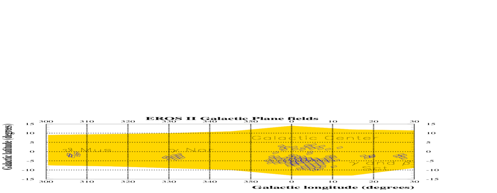 Figure 2: Map of the Galactic plane fields (Galactic coordinates)
monitored by EROS for the microlensing search.
The shaded area represents the shape of the Galaxy.
We have indicated our Galactic Centre fields and the 4
directions towards the arms.
Figure 2: Map of the Galactic plane fields (Galactic coordinates)
monitored by EROS for the microlensing search.
The shaded area represents the shape of the Galaxy.
We have indicated our Galactic Centre fields and the 4
directions towards the arms.
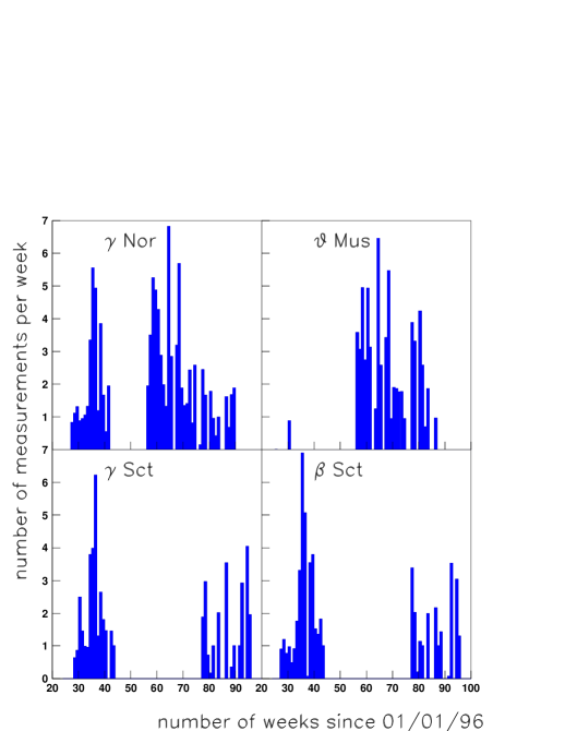 Figure 3: Time sampling for each direction monitored towards the
spiral arms, in number of measurements per week.
Nor is monitored between January and October,
Mus is observed between January and August.
& Sct are monitored between May and November.
By contrast with the Magellanic Clouds,
the distance distribution of the monitored stars is imperfectly known,
and should a priori vary with the limiting magnitude.
In our detection conditions, the populations of stars used
to obtain the optical depths given in Sect. 4.1 below are those
described by the colour-magnitude diagrams of Fig. 4.
An analysis of these diagrams has shown that their content is
dominated by a population of source stars located kpc away,
undergoing an interstellar extinction
of about 3 magnitudes (see Mansoux (1997) for more details).
This distance estimate is in rough agreement with the distance to the
spiral arms deduced from Georgelin et al. (1994) and Russeil et al. (1998),
and will be used in this paper.
Figure 3: Time sampling for each direction monitored towards the
spiral arms, in number of measurements per week.
Nor is monitored between January and October,
Mus is observed between January and August.
& Sct are monitored between May and November.
By contrast with the Magellanic Clouds,
the distance distribution of the monitored stars is imperfectly known,
and should a priori vary with the limiting magnitude.
In our detection conditions, the populations of stars used
to obtain the optical depths given in Sect. 4.1 below are those
described by the colour-magnitude diagrams of Fig. 4.
An analysis of these diagrams has shown that their content is
dominated by a population of source stars located kpc away,
undergoing an interstellar extinction
of about 3 magnitudes (see Mansoux (1997) for more details).
This distance estimate is in rough agreement with the distance to the
spiral arms deduced from Georgelin et al. (1994) and Russeil et al. (1998),
and will be used in this paper.
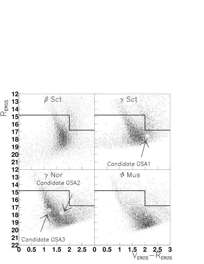 Figure 4: Colour-magnitude diagrams ( vs )
for the stars monitored by EROS in
the directions of & Sct, Nor and Mus.
The boxes drawn in the upper corners correspond to the zones excluded
from the search. The positions of the 3 candidates are indicated.
Figure 4: Colour-magnitude diagrams ( vs )
for the stars monitored by EROS in
the directions of & Sct, Nor and Mus.
The boxes drawn in the upper corners correspond to the zones excluded
from the search. The positions of the 3 candidates are indicated.
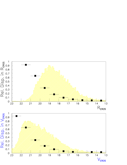 Figure 5: Relative frame to frame average dispersion of the luminosity
measurements versus (upper panel) and
(lower panel), for stars with at least 50 reliable
measurements for each colour.
This dispersion is taken as an estimator of the mean photometric precision.
The superimposed hatched histograms show the magnitude distribution of
the stars in EROS bands.
Figure 5: Relative frame to frame average dispersion of the luminosity
measurements versus (upper panel) and
(lower panel), for stars with at least 50 reliable
measurements for each colour.
This dispersion is taken as an estimator of the mean photometric precision.
The superimposed hatched histograms show the magnitude distribution of
the stars in EROS bands.
 Figure 6: EROS microlensing detection efficiency
as a function of , the Einstein radius crossing time.
is the ratio of
the number of simulated events, satisfying the selection criteria
with duration , with
any and any date of peak magnification within the research
period (650 days),
to the number of events generated with .
Figure 6: EROS microlensing detection efficiency
as a function of , the Einstein radius crossing time.
is the ratio of
the number of simulated events, satisfying the selection criteria
with duration , with
any and any date of peak magnification within the research
period (650 days),
to the number of events generated with .
3 The search for lensed stars


3.1 Data processing and analysis
Light curves have been produced from the sequences of images using the specific software PEIDA (Photométrie et Étude d’Images Destinées à l’Astrophysique), designed to extract photometric information in crowded fields (Ansari (1996)). Figure 5 shows the mean point-to-point relative dispersion of the measured fluxes along those light curves as a function of and . A systematic search for microlensing events has been performed on a set of about 300,000 stars per field ( light curves in total), with an average of 70 measurements in the and colours (between July 1996 and November 1997). This search is based on procedures and criteria similar to the ones developed for the EROS microlensing search in the SMC data (Palanque-Delabrouille et al. (1998)). These criteria are designed to select microlensing events using the expected characteristics of their light curves (one single peak, simultaneous in the visible and red bands, with a known shape), and to reject variable stars (rejection of stars lying in regions of the colour-magnitude diagrams mostly populated by variable stars, and requirement for the stability of the curve outside the peak). They are also tuned to be loose enough to avoid rejection of non-standard microlensing events, which have a different peak shape. The main difference from the SMC analysis is the rejection against variable stars from the instability strip and against red giant variables. Unlike the Magellanic Clouds case where the positions of these populations in the colour-magnitude diagram are known a priori, the scatter and imperfect knowledge of the distances and reddenings of our target stars make our colour-magnitude cut somewhat empirical. In particular, its acceptance is different from one field to another (see the excluded regions in Fig. 4).3.2 The efficiency of the analysis
To determine the efficiency of each selection criterion, we have applied them to Monte-Carlo generated light curves, obtained from a representative sample of the observed light curves, on which we superimpose randomly generated microlensing effects. The microlensing parameters are uniformly drawn in the following intervals: impact parameter expressed in Einstein radius unit , maximum magnification time in a research period starting 50 days before the first observations and ending 50 days after the last observations111Outside this domain of parameters, the detection efficiency is negligible., and Einstein radius crossing time days. The analysis efficiency (or sampling efficiency) shown in Fig. 6 is relative to a set of unblended stars. Blending of a lensed star results in the mixing of unmagnified light with the expected light curve. The efficiency of the search and the reconstruction of the lensing parameters are hence affected by this distortion. On the other hand, the set of stars that could undergo a detectable lensing effect is larger than the sample of the monitored stars, and the expected number of events is also affected. These effects, which are usually included as corrections to the sampling efficiency, are not taken into account in the present article and will require a specific study. For other targets (SMC, LMC), we have determined the correction of the detection rate due to blending to be less than 10-20% (Renault (1996); Palanque-Delabrouille (1997)).3.3 Results of the selection
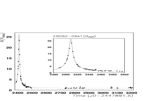
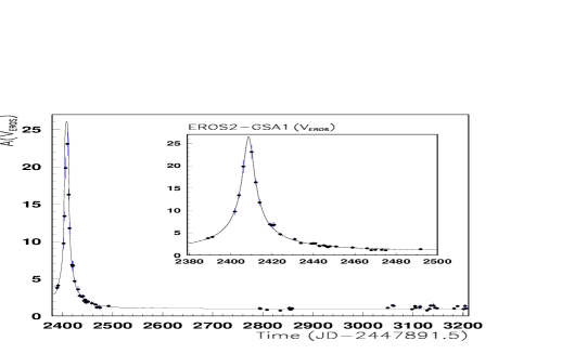
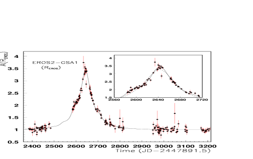
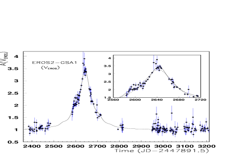
Three light curves satisfy all the requirements and are hereafter named candidates and labelled GSA1 to 3. Figures 7, 8 and 9 show the light curves of each candidate and Table 2 contains their characteristics. Measurements taken after Jan 1st, 1998 (date 2922) are shown, although they were not used in the selection. Table 2: Characteristics of the 3 microlensing candidates Candidate EROS2-GSA1 EROS2-GSA2 EROS2-GSA3 field Coordinates of star (J2000) Galactic coordinates Date of maximum magnification Aug. , 1996 Mar. , 1997 Oct. , 1997 Julian Day -21,447,891.5 Einstein radius crossing time (days) Max. magnification Impact parameter (in ) of best fit 185.7/163 d.o.f. 551/425 d.o.f. 445/427 d.o.f. Remarks binary source fit at 95% C.L. (see text) period 98 days (see text)4 Optical depth and event timescales
4.1 Optical depth
The optical depth towards a pointlike source is defined as the fraction of time during which it undergoes a lensing magnification larger than 1.34. For a given target the measured optical depth is computed from: where is the number of monitored stars in the target, is the duration of the search period (650 days for this 2 year analysis) and is the average detection efficiency normalized to the microlensing events with impact parameter , whose maximum magnification takes place within the research period. The contribution of the candidates to the optical depth is given in Table 3. Table 3: Contribution of the candidates to the optical depth assuming the sources to be away. In the case of Mus we give a 95% C.L. upper limit on the optical depth contribution from events with days ( = 18%). Target Scutum Norma Musca Direction Events detected none GSA1 GSA2 & 3 none (days) - & (80) (%) (18) (event)() - 1.02 - (target)() at 95% CL averaged over the 4 directions () We have modeled the Galaxy in two different ways using three components: a central bulge, a disc and a dark halo. The density distribution for the bulge - a barlike triaxial model - is taken from Dwek et al. (1995) model G2 (in cartesian coordinates): where is the bulge mass, and a, b, c are the length scale factors. The bar major axis is inclined at an angle of with respect to the Sun-Galactic Centre line. We compare our measurements with the predictions of two models with extreme disk contributions (here the main structure involved in microlensing). The first one has a “thin” disc and a standard isotropic and isothermal halo (Model 1) with a density distribution given in spherical coordinates by: where is the local halo density, is the distance between the Sun and the Galactic Centre, and is the Halo “core radius”. The matter distribution in the disc is modeled in cylindrical coordinates by a double exponential (see e.g Bienaymé et al. (1987) and Schaeffer et al. (1998)): is the column density of the disc at the Sun position, is the height scale and is the length scale of the disc. The second model (Model 2) has a “thin” and a “thick” disc, and a very light halo. Both models share the same bulge contribution. The model parameters are summarized in Table 4. Table 4: Parameters of the galactic models used in this article. Parameter Model 1 Model 2 1.49 Bulge 0.58 0.40 2.1 50 Thin disc 0.325 3.5 4.3 - 35 Thick disc - 1.0 - 3.5 - 3.1 0.008 0.003 Halo 5.0 5.0 51 7 0.085 0.098 Predictions 211 222 203 180 200 140 Fig. 1 shows the expected optical depth up to as a function of longitude for both models, at the average latitude of our fields . As the main contribution comes from the thin disc (about 90%), variations of the optical depth from field to field due to the range of to in latitude can reach in the case of Nor, and for the other targets. The expected optical depth, averaged over the four directions, is for model 1, and for model 2. These estimates vary by 50% if the average distance of the sources is changed by 2kpc, or if the parameter is changed by . The measured optical depth, averaged over the four directions is: The confidence interval reported here takes into account Poisson fluctuations and the possible event timescale variations inside the range days. The comparison of Fig. 1 with Table 3 also shows that the measured optical depths in the four directions are compatible with the predictions of both models.4.2 Microlensing event timescales
The duration of the three events is long ( days in average). Fig. 10 shows the expected event duration distribution towards within the framework of model 1. This distribution is obtained assuming the following mass functions and kinematical characteristics: • We assume that lenses belonging to the (non-rotating) halo have the same mass (); their velocities transverse to the line of sight of disc stars follow a Boltzmann distribution with a dispersion of . Thus the expected duration of microlensing events is small (see Fig. 10). • For lenses belonging to the bulge, the mass function is taken from Richer et al. (1992) and the velocities transverse to the line of sight of disc stars also follow a Boltzmann distribution with a dispersion of . The expected rate of microlensing events due to this structure towards the direction considered in Fig. 10 () is found to be negligible. • The disc lenses mass function is taken from Gould (1997), which is derived from HST observations. Disc lenses are subject to a similar global rotation as the observer and the sources (Brand & Blitz (1993)). We assume a negligible particular motion of the monitored sources with respect to the spiral arms, because they are probably young stars. Following Griest (1991), the motion of the Sun relative to the Local Standard of Rest is taken as (in km/s) ; the velocity dispersions of the lens population are expected to be (in km/s). As the disc lenses have a low velocity relative to the line of sight, disc-disc events have longer timescales, as can be seen on Fig. 10. Assuming that all three lenses belong to the halo leads to large probable masses (). As such high mass lenses would be visible stars that we do not observe (dismissing the unlikely possibility that the three could be neutron stars), the disc-disc lensing hypothesis is more probable.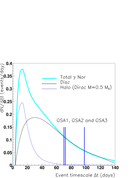 Figure 10: distribution
of the events expected during the search
period per monitored stars towards
, within model 1.
This distribution takes into account
the detection efficiency .
The durations of the three candidates are marked.
Notice that the bulge contribution is negligible.
This hypothesis could also explain
the fact that 4 events over the 45 found by the MACHO
Collaboration towards the Galactic Centre (see Alcock et al. 1997b )
have a timescale days, significantly larger
than the mean for the whole sample (21 days).
Indeed, the contribution of these 4 events to the total optical depth
is about , which is compatible with the expectation
of the disc lensing contribution ( for Model 1).
Figure 10: distribution
of the events expected during the search
period per monitored stars towards
, within model 1.
This distribution takes into account
the detection efficiency .
The durations of the three candidates are marked.
Notice that the bulge contribution is negligible.
This hypothesis could also explain
the fact that 4 events over the 45 found by the MACHO
Collaboration towards the Galactic Centre (see Alcock et al. 1997b )
have a timescale days, significantly larger
than the mean for the whole sample (21 days).
Indeed, the contribution of these 4 events to the total optical depth
is about , which is compatible with the expectation
of the disc lensing contribution ( for Model 1).
5 Detailed analyses of the candidates
Detailed analyses have been performed on GSA1 and GSA2 candidates, whose light curves are sufficiently sampled. For this purpose, we have used all available data on the candidates (i.e. three years of observations).5.1 Candidate EROS2-GSA1
Candidate GSA1 exhibits a large magnification ( at 95% C.L.) with no detectable blending222Fits including more than 10% blending are excluded at 95% C.L. Moreover, since the magnification curves are the same in both colours, the amplified star and an hypothetical blending star would have to have -by chance- the same colour. and no detectable parallax effect (Gould (1992)). Despite the small impact parameter, no evidence for a distortion of the curve due to the non-zero size of the lensed source is found. A fitting procedure allows one to put an upper limit to the ratio of the angular stellar radius to the angular Einstein radius of the lens: where is the lens mass, the distance of the observer to the source and its distance to the lens. From the position of the source in the colour-magnitude diagram we can assume that its temperature is comparable to or lower than that of the Sun. We then obtain: where the apparent magnitude should be corrected for the interstellar extinction. Ignoring this correction leads to the conservative limit , implying that and that the angular proper motion of the deflector: Assuming the interstellar extinction to be 3 magnitudes (see Sect. 2.2) leads to , implying that and: Since the typical expected value (based on Galactic kinematics) is , this limit does not probe the expected range of parameter space. On the other hand, the standard microlensing fit is satisfactory, and taking into account the possibility of a parallax effect does not result in a significantly better fit. We can then infer a lower limit on , the size of the Einstein ring projected from the source onto the observer’s plane: This implies a lower limit on the projected speed of the lens onto the local transverse plane: Since typical values expected for this quantity are of the order of , it is clear that this is not a very constraining limit either. Fig. 11 shows the excluded area for the tip of the 2-dim. vector in the local transverse plane. The lower limit we find for the modulus (and ) is relatively small, because the best parallax fit, which is not significantly better than a standard fit (183.7/161 d.o.f. compared with 185.7/163 d.o.f.), is obtained for in the frame of Fig. 11. This special configuration produces a distorted light curve which diverges only marginally from the standard fitted curve, and only during periods where the measurements are not very precise. From the definitions of and one gets the relation: from which we derive a lower limit on the lens mass by combining the two constraints from finite size and parallax analysis, i.e. at 95% C.L.: Note that this limit is independent of the lens and source distances to the observer. The fact that this lower limit is so much smaller than the expected mass for such lenses follows immediately from the fact that each limit from which it is derived is not probing the expected range of kinematic parameters. Fig. 12 shows the excluded areas in the versus plane, from the finite size study and the parallax analysis, assuming the source to be located kpc away. Exclusion curves for the two hypotheses on the interstellar absorption are shown. A better characterization of the lensed source should allow one to refine these preliminary studies. Finally, a limit on the lens luminosity can be derived from the maximum blending limit allowed by the fit. At 95% C.L., the apparent magnitude of the lens is at least 2.5 magnitudes above the measured baseline magnitude, i.e. and .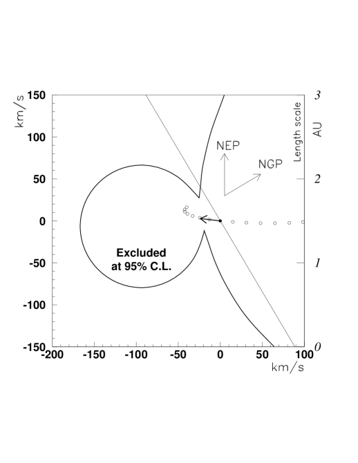 Figure 11: Excluded area for the tip of the 2-dim. vector
in the local transverse plane.
The smallest speed compatible with the observations
corresponds to a deflector with a velocity
oriented towards the lower spike.
The arrow shows the earth projected velocity at the maximum magnification
time.
The straight line is the intersection of the Galactic plane.
The projection of the earth trajectory is indicated by the open circles,
starting 60 days before maximum, ending 70 days after maximum,
with 10 days spacing (right scale in AU).
NEP is the North Ecliptic Pole direction, NGP is the North
Galactic Pole direction.
Figure 11: Excluded area for the tip of the 2-dim. vector
in the local transverse plane.
The smallest speed compatible with the observations
corresponds to a deflector with a velocity
oriented towards the lower spike.
The arrow shows the earth projected velocity at the maximum magnification
time.
The straight line is the intersection of the Galactic plane.
The projection of the earth trajectory is indicated by the open circles,
starting 60 days before maximum, ending 70 days after maximum,
with 10 days spacing (right scale in AU).
NEP is the North Ecliptic Pole direction, NGP is the North
Galactic Pole direction.
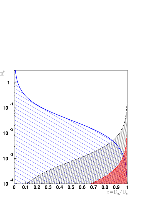 Figure 12: 95% C.L. exclusion diagram from the parallax analysis
and from the finite source size study for the candidate EROS2-GSA1.
The lower curve in the right part is the conservative limit
ignoring interstellar absorption, the higher curve corresponds
to a 3 magnitude absorption.
These curves assume the source to be located
away. If the source is assumed to be at some other distance , one
has to scale the increasing functions by the factor ,
and the decreasing function by .
Figure 12: 95% C.L. exclusion diagram from the parallax analysis
and from the finite source size study for the candidate EROS2-GSA1.
The lower curve in the right part is the conservative limit
ignoring interstellar absorption, the higher curve corresponds
to a 3 magnitude absorption.
These curves assume the source to be located
away. If the source is assumed to be at some other distance , one
has to scale the increasing functions by the factor ,
and the decreasing function by .
5.2 Candidate EROS2-GSA2
GSA2 has residuals to a standard microlensing fit which clearly exhibit a modulation; a period of days is found in the residuals of the standard fit during the magnification. On the other hand, taking into account a possible parallax effect does not significantly improve this fit. Furthermore, we know that the lensing of a periodic variable star would produce a modulation of the light curve whose amplitude should follow the magnification. As we do not detect a significant modulation in the non-magnified part of the light curve, the most probable origin of this modulation is that one dominant luminous source or two sources orbit around the centre of gravity of a binary system, inducing a wobbling of the line of sight with respect to the trajectory of the lens 333This type of configuration has been studied by Griest & Hu (1992), Sazhin & Cherepashchuk (1994) and Han & Gould (1997), and was already mentioned in our earlier article (Ansari et al. (1995)).. In this configuration, a modulation of the light curve is expected to occur only during the lensing peak. We obtain equally satisfactory fits for two classes of circular binary systems (with at best for 425 d.o.f., to be compared with 876 for 439 d.o.f. for a standard microlensing fit). The first class includes systems with a dominant source orbiting with a period days, and with the projected semi-axis 444Fits which are slightly less good can be obtained with larger periods, but in this case only the first shoulder (around date=2600) is correctly matched.. The second class corresponds to systems with two luminous stars orbiting with a period days, with luminosity and mass ratios around 1/3-1/2, and a projected distance between the two components of about . Given the domain of values for and , these parameters are compatible with physically acceptable masses of the binary satisfying Kepler’s third law. Many more configurations can fit the observations if we consider systems with elliptic orbits. Figure 13: Relation between and assuming
a binary system with , and a total mass
of or .
Figure 13: Relation between and assuming
a binary system with , and a total mass
of or .
A spectroscopic study of the source is under way in order to test its binarity. If the source proves to be a spectroscopic binary, then one can get a good estimate or constraint on the angular Einstein radius (and then on the angular proper motion of the lens ). Expressing the Einstein radius and Kepler’s third law in the relation leads to: Fig. 13 illustrates this relation between and assuming the source to be a binary system with days, with and with two different hypotheses for the mass of the system.
6 Conclusion
We have searched for microlensing events with durations ranging from a few days to a few months in four Galactic disc fields lying to from the Galactic Centre. We find three events that can be interpreted as microlensing effects due to massive compact objects. Their long duration favours the interpretation of lensing by objects belonging to the disc instead of the halo. The average optical depth measured towards the four directions is . Assuming the sources to be away, the expected optical depths from two different galactic models vary from to , in agreement with our measurement. One event displays a modulation of the magnification which is compatible with the lensing of a binary source. More information about the configuration of this possible binary source, and about the lens mass acting on the strongly amplified source, are expected from complementary observations. No evidence for parallax and blending effects has been found. The observations continues towards the spiral arms. More accurate measurements should be obtained with the increase of statistics (Derue (1999)), allowing one to estimate the disc contribution to the optical depth towards the bulge and the Magellanic Clouds.Acknowledgements.
We are grateful to D. Lacroix and the technical staff at the Observatoire de Haute Provence and to A. Baranne for their help in refurbishing the MARLY telescope and remounting it in La Silla. We are also grateful for the support given to our project by the technical staff at ESO, La Silla. We thank J.F. Lecointe for assistance with the online computing. We wish to thank also C. Nitschelm for his contribution to the data taking.References
- Alcock et al. (1993) Alcock C., Akerlof C.W., Allsman R.A. et al. (MACHO Coll., 1993, Nat 365, 621.
- Alcock et al. (1995) Alcock C., Allsman R.A., Axelrod T.S. et al. (MACHO Coll.), 1995, ApJ 445, 133.
- (3) Alcock C., Allsman R.A., Alves D. et al. (MACHO Coll.), 1997a, ApJ 486, 697.
- (4) Alcock C., Allsman R.A., Alves D. et al. (MACHO Coll.), 1997b, ApJ 479, 119.
- Alcock et al. (1998) Alcock C., Allsman R.A., Alves D. et al. (EROS Coll., MACHO Coll.), 1998, ApJ 499, L9.
- Ansari (1996) Ansari R., 1996, Vistas in Astronomy 40, 519
- Ansari et al. (1995) Ansari R., Cavalier F., Couchot F. et al. (EROS Coll.), 1995, A&A 299, L21.
- Ansari et al. (1996) Ansari R., Cavalier F., Moniez M. et al. (EROS Coll.), 1996, A&A 314, 94.
- Aubourg et al. (1993) Aubourg É., Bareyre P., Bréhin S. et al. (EROS Coll.), 1993, Nat 365, 623.
- Bauer et al. (1997) Bauer F., Afonso C., Albert J-N et al. (EROS Coll.), 1997, Proceedings of the “Optical Detectors for Astronomy” workshop, ESO.
- Bienaymé et al. (1987) Bienaymé O., Robin A., Crézé M., 1987, A&A 180, 94.
- Brand & Blitz (1993) Brand J., Blitz L., 1993, A&A 275, 67.
- Derue (1999) Derue F., 1999, Ph.D. thesis, CNRS/IN2P3, LAL report 99-14, Université Paris XI Orsay.
- Dwek et al. (1995) Dwek E., Arendt R.G., Hauser M.G. et al., 1995, ApJ 445, 716.
- Georgelin et al. (1994) Georgelin Y.M, Amram P., Georgelin Y.P. et al., 1994, A&AS 108, 513.
- Gould (1992) Gould A., 1992, ApJ 392, 442.
- Gould (1997) Gould A., Bahcall J.N., Flynn C., 1997, ApJ 482, 913.
- Griest (1991) Griest K., 1991, ApJ 366, 412.
- Griest & Hu (1992) Griest K., Hu W., 1992, ApJ 397, 362.
- Han & Gould (1997) Han C., Gould A., 1997, ApJ 480, 196.
- Mansoux (1997) Mansoux B., 1997, Ph.D. thesis, CNRS/IN2P3, LAL report 97-19, Université Paris 7.
- (22) Paczyński B., 1986, ApJ 304, 1.
- Palanque-Delabrouille (1997) Palanque-Delabrouille N., 1997, Ph.D. thesis, CEA DAPNIA/SPP report 97-1007, Université Paris 7.
- Palanque-Delabrouille et al. (1998) Palanque-Delabrouille N., Afonso C., Albert J-N. et al. (EROS Coll.), 1998, A&A 332, 1.
- Renault (1996) Renault C., 1996, Ph.D. thesis, CEA DAPNIA/SPP report 96-1003, Université Paris 7.
- Richer et al. (1992) Richer H.B., Fahlman G.G., 1992, Nature 358, 383.
- Russeil et al. (1998) Russeil D., Amram P., Georgelin Y.P. et al., 1998, A&AS 130, 119.
- Sazhin & Cherepashchuk (1994) Sazhin M. V., Cherepashchuk A. M., 1994, Astron. Lett., Vol. 20, No. 5, 523.
- Schaeffer et al. (1998) Schaeffer R., Méra D. and Chabrier G., 1998, Acta. Phys. Polonica B., Vol. 29, 1905.
- Udalski et al. (1993) Udalski A., Szymański M., Kaluzny J. et al. (OGLE Coll.), 1993, Act. Astr. 43, 289.
- Udalski et al. (1994) Udalski A., Szymański M., Stanek K.Z. et al. (OGLE Coll.), 1994, Act. Astr. 44, 165.