Multiwavelength Properties of Blazars

Abstract

Blazar spectral energy distributions (SEDs) are double peaked and follow a self-similar sequence in luminosity. The so-called “blue” blazars, whose first SED component peaks at X-ray energies, are TeV sources, although with a relatively small fraction of their bolometric luminosities. The “red” blazars, with SED peaks in the infrared-optical range, appear to emit relatively more power in the gamma-ray component but at much lower energies (GeV and below). Correlated variations across the SEDs (of both types) are consistent with the picture that a single electron population gives rise to the high-energy parts of both SED components, via synchrotron at low energies and Compton-scattering at high energies. In this scenario, the trends of SED shape with luminosity can be explained by electron cooling on ambient photons. With simple assumptions, we can make some estimates of the physical conditions in blazar jets of each “type” and can predict which blazars are the most likely TeV sources. Upper limits from a mini-survey of candidate TeV sources indicate that only $\sim 10$% of their bolometric luminosity is radiated in gamma-rays, assuming the two SED components peak near 1 keV and 1 TeV. Finally, present blazar samples are too shallow to indicate what kinds of jets nature prefers, i.e., whether the low-luminosity “blue” blazars or the high-luminosity “red” blazars are more common.

1 The Blazar Paradigm

1.1 SEDs and variability

The spectral energy distributions (SEDs) of blazars have two components, with peaks (in the usual $\nu F_{\nu}$ representation) separated by $\sim 8-10$ decades in frequency, as discussed by [34, 8] and several authors in this volume. The lower frequency component has peak frequency, $\nu_{p}$, in the IR-X-ray energy range, and is generally believed to be due to synchrotron radiation, so the peak can be identified with a characteristic electron energy $\gamma_{peak}\propto\sqrt{\nu_{peak}/B}$. Typically blazars are more variable — more rapidly and with larger amplitude — at or above the spectral peak, certainly in the synchrotron component and plausibly in the gamma-ray component, although here the data are much more sparse.

The variability in the two blazar spectral components is correlated, with wavelength-dependent lags, between approximately corresponding points on the two curves ([34]). This has led to the suggestion that a single population of electrons could be responsible for the bulk of the emission in both components, via synchrotron radiation in the low energy bump and via Compton scattering of local soft photons in the high energy bump. (Other components contribute to the extended radio emission and to an optical/UV bump, if present.) For the remainder of the talk, I refer to “synchrotron” and “Compton” spectral components, but recognize that for the high-energy emission at least, there are other still-plausible models.

As others discuss at this conference, the origin of the seed photons for the Compton-scattered gamma-rays has been a subject of some speculation. Different possibilities include local synchrotron photons produced by the same electron population (the SSC model, [22]), or sources external to the jet, such as accretion disk photons ([6]) or reprocessed photons from the broad-line region ([31]). Quite possibly the relative importance of these possibilities changes from one source to the next, or between active and quiescent periods in a given source, as the intrinsic source properties change ([12]).

There are clues in the trends in blazar properties with luminosity. Rita Sambruna showed in her Ph.D. thesis that synchrotron peak frequencies and overall spectral shapes differed among X-ray-selected BL Lac objects, radio-selected BL Lac objects, and flat-spectrum radio quasars ([29]), in a way that could not be explained simply by beaming. Instead, the SEDs changed shape systematically with luminosity, such that high luminosity BL Lac objects and quasars have synchrotron peaks in the IR-optical, while lower luminosity BL Lacs peak at higher energies, typically UV-X-ray. We refer to these as LBL (for low-frequency peaked blazars) and HBL (for high-frequency peaked blazars), respectively (see [23] for exact definition), or more descriptively, as “red” and “blue” blazars. BL Lacs found in the first X-ray surveys were generally HBL/blue; BL Lacs found in classical radio surveys were generally LBL/red, as were most FSRQ (flat-spectrum radio-loud quasars), though “bluer” FSRQ are now being identified in multiwavelength surveys designed not to exclude them ([25, 20]).

Table 1: Spectral Trends in Blazars

as $L_{bolometric}$ increases,	$\nu_{synchrotron}$ decreases
	$L_{Compton}$ increases
	$L_{\rm emission-line}$ increases
$\nu_{Compton}/\nu_{synchrotron}$ roughly similar in HBL, LBL, FSRQ

Taking a synthetic view of the origin of the SEDs, it seems the bright EGRET blazars, which have peak gamma-ray emission near $\sim 1$ GeV, are much like the few known TeV blazars, which peak $\lower 2.15277pt\hbox{$\;\buildrel>\over{\sim}\;$}100$ times higher in energy. This is important because many more “GeV” blazars are known and have been studied than “TeV” blazars. With appropriate scaling, we should be able to use the observed behavior of the GeV blazars (see [41]) to inform our multiwavelength studies of TeV blazars (discussed below and see [32]).

1.2 Compton cooling

The SED trends support a simple paradigm ([8, 11]) in which electrons in higher luminosity blazars suffer more cooling because of larger external photon densities in the jet (as indicated by the higher $L_{\rm emission-line}$ characteristic of this group). This leads naturally to lower characteristic electron energies, as well as larger ratios of inverse Compton to synchrotron luminosity ($L_{C}/L_{s}$) because of the “external Compton” (EC) contribution. In contrast, lower luminosity blazars are dominated by (weaker) SSC cooling, and so have electrons with higher $\gamma_{peak}$. The correlation of $\gamma_{peak}$ with energy density may even suggest that electron acceleration in blazars is independent of luminosity, and that only the cooling differs ([11, 13]). A similar luminosity-linked scheme, with a somewhat more physical motivation, was developed by Markos Georganopoulos in his Ph.D. thesis ([10]). In any case, the current view is that the EC process dominates the gamma-ray production in high-luminosity blazars, while the SSC process dominates in low-luminosity blazars. The X-rays from either high- or low-luminosity blazars are likely dominated by SSC ([19, 32]).

The similarity of $\nu_{C}/\nu_{s}$ in HBL and FSRQ/LBL is somewhat puzzling in this picture, and will be physically important if it persists when (if?) further TeV observations define the HBL Compton peaks well (this is complicated by the effect of the Klein-Nishina cross section at TeV energies). In a simple homogeneous SSC model, $\nu_{C}/\nu_{s}\propto\gamma_{peak}^{2}$, whereas in the simplest EC models $\nu_{C}/\nu_{s}\propto\nu_{E}/B$, where $\nu_{E}$ is the characteristic frequency of the external seed photons. If $\nu_{C}/\nu_{s}$ changes little from SSC-dominated to EC-dominated blazars, then perhaps energy is distributed so that the typical electron energy, which depends on acceleration, cooling, and escape, maintains the appropriate relation to the magnetic field energy density.

1.3 Caveats

Two caveats to this scheme bear mentioning, as both can lead to higher observed $L_{C}/L_{s}$ in high-luminosity blazars, even when there are no significant intrinsic differences. First, Dermer has pointed out that EC gamma-rays are more tightly beamed than SSC. Therefore, if the EC process dominates the gamma-ray emission in high-luminosity blazars but the SSC process dominates in low-luminosity blazars, the increase of $L_{C}/L_{s}$ with luminosity will be exaggerated (and could even be spurious).

Second is a sort of “variability bias” (see [39, 15]). Given the limited sensitivity of EGRET, which typically had to integrate for one or more weeks to detect a blazar, this bias arises if two plausible assumptions hold: (1) high-luminosity sources are larger than low-luminosity sources, and their intrinsic variability time scales are proportionately longer, and (2) blazar gamma-ray light curves are characterized by flares separated by quiescent periods, as suggested by the long-term EGRET light curve of 3C 279 ([14]). Scaling from 3C 279, even as slowly as $L^{-1/2}$, a typical EGRET observation would span several flares in a low-luminosity blazar, sampling an average flux close to the quiescent value, hence implying a weak gamma-ray source. In contrast, a high-luminosity source like 3C 279 would be observed either during a flare, in which case it would appear quite luminous, or else tend to be undetected. Indeed, many bright LBLs have never been detected with EGRET. (Note that high-luminosity blazars have a higher average redshift than low-luminosity blazars, due to their lower space density, and so are less likely to be close enough to detect during quiescent periods.)

The net effect of measuring systematically much-higher-than-average gamma-ray luminosities in high-luminosity blazars, and roughly-average-quiescent gamma-ray luminosities in low-luminosity blazars, is to produce the observed trend of $L_{C}/L_{s}$ with $L_{bol}$, at least qualitatively. In the well-known multi-epoch SED of 3C 279 (e.g., [40, 41]), this is seen explicitly: during the highest state, the Compton ratio is between 10 and 100, while during the lowest state, it is 1 or perhaps less (it is poorly determined because the synchrotron peak for this source is in the far-IR and was seldom observed in the key multiwavelength campaigns).

Thus both biases, the greater beaming for EC compared to SSC, and the tendency to detect single flares versus multiple flares depending on luminosity, lead in the same direction, toward higher Compton ratios in high-luminosity sources. Whether these biases can explain the observed trend quantitatively is not yet clear, but they need to be evaluated in within the context of any blazar paradigm (necessarily in a model-dependent way).

2 Properties of TeV-Bright Blazars

2.1 What is known so far

What then are the general properties of the TeV-bright blazars? So far, only two, Mkn 421 and Mkn 501, have been studied in detail, and few additional sources have been reported (1ES 2344+514, [4]; PKS 2155–304, [5]; 1ES 1959+050, [17]). With only two sources reported more than once in the literature, we know little about TeV blazars as a class.

The SEDs of the two well-studied TeV-bright blazars have the usual shape for blue blazars. For Mkn 421, the synchrotron peak is at or slightly above 10¹⁷ Hz, and the Compton peak (including the effect of the Klein-Nishina cross section, which suppresses the Compton component at lower frequencies than would be the case in the Thomson limit) occurs just below 1 TeV. The observed Compton ratio is $\lower 2.15277pt\hbox{$\;\buildrel>\over{\sim}\;$}1$ ([33]). Mkn 501 is slightly different, with a typically lower Compton ratio, although this impression is strongly influenced by the bright flare in spring 1997, when the synchrotron peak increased to $\sim 100$ keV ([26, 3, 1]).

Note that, as [33] shows so clearly, the TeV emission comes largely from low-energy electrons scattering low-energy photons (below the synchrotron peak), with high-energy electrons (those with $\gamma_{e}>\gamma_{peak}$) contributing to a hard tail above the Compton peak. This means the TeV emission reflects closely the electron spectrum and variability, and is relatively insensitive to changes in the seed photon flux (which changes slowly at frequencies below the synchrotron peak; [34]).

2.2 HEGRA survey

Following the general paradigm, we expect blazars with high-energy synchrotron peaks, the HBL/blue blazars, to be bright at TeV energies. Accordingly, we undertook a survey with HEGRA of likely TeV candidates (with Ron Remillard and Felix Aharonian), starting from a list of X-ray-peaked, X-ray-bright, nearby BL Lacs. (A few LBL, typically well-known BL Lacs, were also observed.) Because these sources are X-ray bright, they are detectable with the RXTE All Sky Monitor (ASM), at least in their higher states. If these objects are like Mkn 421, then the 2-10 keV X-ray emission is near the peak synchrotron output and the TeV emission is near the peak Compton output; thus, the HEGRA measurements are a probe of the Compton ratio. Our goal was to measure this ratio, or a limit to it, for blazars generally.

In the end, we observed 10 sources, including 7 HBL and 3 LBL. None were detected and there are only upper limits for the TeV flux ([28]). Because HEGRA sensitivity is $\sim 10^{-11}$ ergs cm^-2 s^-1 and ASM sensitivity is $\sim 10^{-10}$ ergs cm^-2 s^-1, we can in principle, using simultaneous ASM observations, probe an interesting regime in Compton ratio, as low as $L_{C}/L_{s}\sim 1/10$. Unfortunately, six of the sources were also below the ASM detection limit at the epoch of the HEGRA observations, thus we have only four estimates of the Compton ratio, from 3 HBL and 1 LBL (see Fig. 1). The best estimates of the ratios all lie well below 1, closer to 0.1 or 0.2. The 95% confidence upper limits range from 0.35 down to 0.18. Either the typical ratios in blazars are below 1, or the spectra of these four objects differ from Mkn 421. Specifically, if the 2-10 keV ASM band is near the peak of the synchrotron component but the 1-10 TeV HEGRA band lies above the peak of the Compton component, then the measured limit underestimates the Compton ratio.

Figure 1: Upper limits to the Compton ratio, $L_{C}/L_{s}$, of X-ray bright blazars. The average value is significantly below unity, implying that a relatively small fraction of the bolometric luminosity is typically radiated in gamma-rays, at least in the quiescent state. Estimated from HEGRA upper limits ([28]) and simultaneous RXTE ASM fluxes, assuming the Compton and synchrotron peaks lie near 1 TeV and 1 keV, respectively.

From this limited survey we infer that the typical Compton ratios of TeV-bright blazars may be closer to $L_{C}/L_{s}\sim 0.1$ than $\sim 1$. This implies different source parameters than for Mkn 421, for which $L_{C}/L_{s}$ is usually $\sim 1$. For example, [33] derived constraints on the magnetic field and the Doppler factor of Mkn 421 in the context of a simple homogeneous emitting volume. If the value of $L_{C}/L_{s}$ is lower by a factor of $\sim 10$, the magnetic field and/or the Doppler factor must be higher by a factor of a few.

2.3 Directions for future TeV surveys

Our TeV survey was limited not by the lack of HEGRA detections but by the lack of simultaneous X-ray detections (the ASM is a factor of a few less sensitive than required). In the future, in order to estimate the Compton ratio in an unbiased way, the most fruitful approach would be to dedicate pointed RXTE or SAX or ASCA observations to a well-chosen HBL sample, observing simultaneously in the TeV. X-ray detection would be assured, so that any TeV limit would be significant, and the X-ray spectra would allow determination of the synchrotron peak, so the TeV limits could be interpreted with less ambiguity.

Alternatively, to improve the chances of a TeV detection, one could make the plausible link between X-ray flaring and TeV flaring, as observed explicitly in Mkn 421 and Mkn 501, and thus try to trigger on X-ray flares. From the ASM data (http://space.mit.edu/XTE/ASM_lc.html) it is clear that many blazars have relatively short-lived high states. Thus one would need to trigger with very little delay, perhaps responding within 1 day to ASM detections of bright states. With the automated state of data processing in the ASM, such rapid notification to TeV observers should be routinely possible.

2.4 New observations of Mkn 421 in spring 1998

Since Mkn 421 is a very bright source at X-ray and TeV energies, it is an obvious target for monitoring, even recognizing that the results are likely biased toward the flaring state. When RXTE ASM data indicated that Mkn 421 was flaring in February 1997, we triggered a Target of Opportunity (TOO), observing roughly every 10 days with the RXTE PCA through July 1998, with a few additional observations in August 1998. Daily less-sensitive X-ray observations are available from the ASM. During much of this time HEGRA (and other TeV telescopes) were also observing, except during bright time. Figure 2 shows the X-ray and TeV light curves.

Figure 2: X-ray and TeV light curves of Mkn 421 during a flaring state in spring 1998 (MJD 50800 is 1997 December 28). X-ray data are from the RXTE Proportional Counter Array (PCA), obtained during a TOO monitoring program with Ron Remillard, PI, and the RXTE All-Sky Monitor (ASM). Simultaneous HEGRA data are reproduced here with permission (HEGRA collaboration, to be published).

In the X-ray, the PCA (filled circles) detects short time scale variability, while the light curve of daily ASM averages (open circles) samples the longer time scale variability; the two agree well. In early June 1998 (around MJD 50970), the PCA light curve shows a steep decline in X-ray flux, by more than a factor of 2 in 5 hours.

The TeV and X-ray fluxes appear well correlated, consistent with the zero lag (within 1 day) found from more extensive X-ray and TeV light curves of Mkn 421 ([18]). With additional TeV data from the June 1998 flare, it should be possible to comment on lags at shorter time scales. This is certainly in accord with the blazar paradigm discussed above, where a single electron population produces the X-rays via synchrotron radiation and the TeV emission via Compton scattering of soft photons (probably low-frequency synchrotron radiation).

2.5 Multiwavelength observations of the well-studied BL Lac object PKS 2155–304

Only a handful of blazars have been well-monitored simultaneously in multiple spectral bands, the GeV-bright blazar 3C 279 and a few others, and the TeV-bright blazars Mkn 421 and PKS 2155–304. While Mkn 421 has also been monitored at TeV energies (and presumably PKS 2155–304 will be as well now that southern Cerenkov telescopes are coming on line), PKS 2155–304 has probably the best simultaneous data at optical through X-ray energies, which is to say at the high energy end of the synchrotron component.

There have been four extensive multiwavelength campaigns to observe PKS 2155–304 with multiple satellites. In November 1991 ([7]), Rosat (soft X-ray) and IUE (UV and optical) light curves showed closely correlated variations of modest, wavelength-independent amplitude ($\lower 2.15277pt\hbox{$\;\buildrel<\over{\sim}\;$}30$%), with the X-rays leading the UV by a few hours. A second campaign in May 1994 using ASCA, Rosat, EUVE, IUE (without the optical data), and ground-based telescopes showed altogether different results: a strong isolated flare in each band, with much larger amplitude at shorter wavelengths, and with 1-day delays between X-ray and EUV, and between EUV and UV wavelengths ([35]). While such disparate behavior might intuitively suggest quite different properties in the emitting plasma, in fact, [9] explain much of the observed multiwavelength behavior starting from the same underlying jet and varying only the electron injection event.

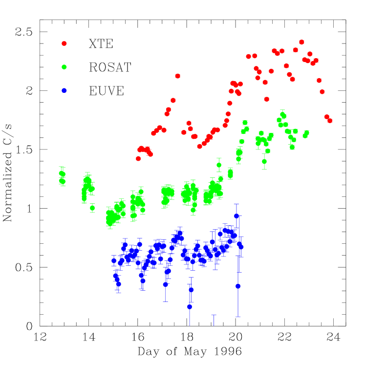
Figure 3: Multiwavelength light curves of the TeV blazar PKS 2155–304 in May 1996 ([30]). Each band is normalized to its own average, then plotted with arbitrary offset, with XTE at the top, ROSAT in the middle, and EUVE below. As has been seen before, the amplitude increases with energy and variations are generally well correlated, with little or no lag. However, the large flare seen with XTE on May 17, which appears less prominently in the EUVE light curve, has no counterpart in the ROSAT light curve. The light curves of PKS 2155–304 in this third multiwavelength campaign differ significantly from those in both the first and second campaigns ([7, 35], obviating simple interpretations of any one multiwavelength data set.

A third multiwavelength monitoring campaign in May 1996, involving RXTE, Rosat, and EUVE (and lacking IUE because of a spacecraft failure a few weeks earlier) shows yet another result ([30, 38]), shown in Figure 3. The RXTE PCA and Rosat PSPC light curves are well correlated in the second half of the 12-day observation, with little or no lag, but near the beginning, a large flare in the RXTE data is not seen in the Rosat data (although there is a small gap in the ROSAT data). A fourth campaign, in November 1996, with RXTE and Rosat, again shows good correlation as far as the more limited data allow ([30, 38]).

These disparate results illustrate the danger of drawing strong conclusions from single-epoch multiwavelength campaigns, not to mention the danger of extrapolating from one or two sources to all blazars.

2.6 The unusual spectral behavior of Mkn 501

Others have referred to the extraordinary flaring of Mkn 501 in April 1997, with strong TeV flux and X-ray spectrum hardening in a previously unobserved way ([26, 3]). Pian and collaborators observed Mkn 501 again with BeppoSAX in April 1998, and found that while the X-ray flux remained quite high and was similar to that seen in April 1997, the synchrotron peak was at $\sim 10$-20 keV, still harder than typical but a factor of $\sim 10$ lower in energy than at the peak of the 1997 flare ([27]).

Thus the characteristic electron energy is somewhat lower but there is clearly ongoing acceleration, sustained over more than one year, as evidenced by the continuous RXTE ASM light curves. Apparently the time scales in Mkn 501 are longer than in Mkn 421, at least at the present epoch, despite their similar luminosities and spectral properties.

3 What Kind of Jets Does Nature Make?

3.1 The extrema of jet physics

We have described how the spectral energy distributions of blazars differ markedly between the low-luminosity sources discovered primarily in X-ray surveys and the high-luminosity sources discovered primarily in radio surveys. Whether the origin of the SED differences is due to electron cooling or something else, inevitably the jet physics in the two types of blazar must differ. In fact, given the selection biases, there must be a distribution of SEDs, and therefore a range of typical electron energies and/or jet physics, as indeed has been found recently in surveys selected to favor intermediate objects ([20, 25]).

Clearly nature makes jets with a range of properties. Perhaps the process of jet formation varies, or the effect of circumnuclear environment affects the eventual jet properties, or some combination of the two (e.g., [2]). Since jet formation is a fundamental question, it is of considerable interest to understand the IMF, as it were, of jets.

3.2 Number densities of red and blue blazars

In fact, the relative number of red blazars and blue blazars is very poorly known ([36]). X-ray surveys, which find the blue blazars because of their high-frequency synchrotron peaks, span a large range in flux but a relatively small range in luminosity. Radio surveys, which pick out red blazars because of their low-frequency peaks, span a small range in flux but a rather larger range in luminosity. Both are undoubtedly biased, but to find the absolute numbers of blue or red blazars requires correcting either type of survey for the kind of objects not found in that survey.

Deriving the relative density of types of blazars is inevitably a model-dependent process. Figure 4 illustrates the dilemma with two extreme cases. If one assumes that X-ray surveys are unbiased, then the numbers of X-ray sources is reflected in the source counts, here taken from a number of surveys at different flux limits (left panel). To compare the density of red blazars, we convert the radio counts to X-ray counts via the average value of $\alpha_{rx}$ appropriate to this sample ([37]), and plot these also in the left panel of Figure 4. The values of $\alpha_{rx}$ are quite steep (the X-ray fluxes are low) so the radio counts lie on the low-flux left side of the plot. This representation of the source counts suggests red blazars are 10 times less numerous than blue blazars. This is certainly the case for a given X-ray flux but would be true in a bolometric sense only if the SEDs of red and blue blazars were the same, which we know very well they are not.

Figure 4: The X-ray and radio number counts for blue (open symbols) and red (filled symbols) BL Lac objects illustrate the ambiguity over which population is more numerous. Left — Observed X-ray counts for X-ray-selected samples are $\sim 10$ times higher than the “bivariate” X-ray counts for radio-selected samples (radio-derived surface density combined with observed X-ray fluxes; [37]). Right — Beaming model extrapolation (solid line) of observed radio counts for radio-selected samples ([36]) is $\sim 10$ times higher than the “bivariate” radio counts for X-ray-selected samples (X-ray-derived surface density combined with the observed radio fluxes).

Alternatively, one can assume the radio survey is unbiased, and compare surface densities of red and blue blazars starting from the 1 Jy and S4 surveys. In this case, the X-ray samples are converted to radio fluxes using the average $\alpha_{rx}$ appropriate to this sample (quite flat, so leading to low radio fluxes). Here the flux ranges do not overlap at all, but using the extrapolation implied by the best-fit beaming model ([24, 37]; solid line in both panels), we would conclude that the radio-selected red blazars are 10 times less numerous than the X-ray-selected blue blazars. The truth probably lies between these two extreme views, but at present it is not constrained.

This has of course been explored in much greater detail, starting from luminosity functions that agree with observation, making some assumptions, and calculating absolute numbers ([23, 8]). We can say that the simple picture wherein blue blazars are seen at larger angles to the line of sight than red blazars, on average ([21]) does not explain the full range of SEDs (cf. [10]), and thus the implication that blue blazars are more numerous (due to their larger solid angle) does not seem to be correct. On the other hand, the assumption that the radio is unbiased ([23]) and that there is a distribution of spectral cutoffs does explain the observed X-ray and radio counts, but the calculation is entirely symmetric with respect to wavelength. One can equally well assume that the X-ray is unbiased, and that there is a range of spectral cutoffs toward longer wavelengths, and again the X-ray and radio counts can be matched.

This ambiguity results because present samples are small and, particularly in the radio, have relatively high flux limits. Even slightly more sensitive radio surveys should be able to verify or disprove these two contradictory hypotheses.

4 Summary

A viable blazar paradigm can be constructed from the observed multiwavelength properties of blazars. All blazars would have synchrotron and inverse-Compton-scattered components, with external seed photons dominating the gamma-ray component in high-luminosity sources (the EC model) and synchrotron seed photons dominating in low-luminosity sources (the SSC model). In both cases, the X-rays are likely to be dominated by Compton-scattered synchrotron (SSC) photons.

Empirical relations between source parameters and luminosity suggest electron acceleration may be universally the same independent of luminosity, whereas cooling is strongly luminosity-dependent. The more luminous sources, with their high ambient photon densities, have much greater cooling and therefore lower average electron energies, and therefore lower frequency synchrotron and Compton peaks, as well as higher ratios of Compton to synchrotron radiation. Several selection effects could exaggerate this trend, however.

The multiwavelength properties of TeV-bright blazars are beginning to be well studied. However, the average properties of blue blazars may be different from those of the well-studied TeV blazars Mkn 421 and Mkn 501. For example, a small survey with HEGRA suggests the typical Compton ratio may be closer to $L_{C}/L_{s}\sim 0.1$ than 1. Further TeV observations, combined with more sensitive simultaneous X-ray observations, are needed to confirm this suggestion. In addition, X-ray monitoring can be used to pick out flaring blazars as potentially strong TeV sources; however the trigger times needed are quite short, less than 1 day. Certainly in Mkn 421 and Mkn 501, the TeV and X-ray light curves are well correlated, with delays $\;\buildrel<\over{\sim}\;$ day.

PKS 2155–304, perhaps the best observed blazar at UV-X wavelengths, illustrates the complexity of blazar variability and the danger of strong conclusions from limited data sets. Mkn 501 continues to be in a high state but $\gamma_{peak}$ has decreased, judging from synchrotron peak frequency, which is a factor of $\sim 10$ lower than one year earlier.

Finally, jet demographics are an interesting and not yet well understood issue. Whether nature forms more high-luminosity jets than low-luminosity jets, as implied if red blazars are more numerous, or the opposite, is unclear and is of fundamental physical significance. This problem can be approached with deeper samples of flat-spectrum radio sources.

Acknowledgements — It is a pleasure to thank my blazar colleagues, particularly those with whom I have worked most closely in the past year, Riccardo Scarpa, Rita Sambruna, Ron Remillard, Elena Pian, Laura Maraschi, Gabriele Ghisellini, Giovanni Fossati, Annalisa Celotti, and Felix Aharonian, and to acknowledge the warm hospitality of the Center for Astrophysical Sciences at the Johns Hopkins University and the Brera Observatory of Milan during my sabbatical. We thank the HEGRA collaboration for permission to use the Mkn 421 data in advance of publication. This work was supported in part by NASA grants NAG5-3313 and NAG5-3138.

References

- [1] F. Aharonian et al., Astr. Ap. 327 (1997) L5.
- [2] G.V. Bicknell, Ap.J.Supp. 101 (1995) 29.
- [3] M. Catanese et al., Ap.J. 487 (1997) L143.
- [4] M. Catanese, et al., Ap.J. 501 (1998) 616.
- [5] P.M. Chadwick, et al. Ap.J. (1999) in press (astroph 9810209).
- [6] Dermer, C.D., Schlickeiser, R. Ap.J. 416 (1993) 458.
- [7] R.A. Edelson, et al., Ap.J. 438 (1995) 120.
- [8] Fossati, G., Celotti A., Ghisellini G., Maraschi L. M.N.R.A.S. 289 (1997) 136.
- [9] M. Georganopoulos, A.P. Marscher, Ap.J. 506 (1998) 11.
- [10] M. Georganopoulos, A.P. Marscher, Ap.J. 506 (1998) 621.
- [11] G. Ghisellini, A. Celotti, G. Fossati, L. Maraschi, A. Comastri, M.N.R.A.S. 301 (1998) 451.
- [12] Ghisellini, G., Madau, P. M.N.R.A.S. 280 (1996) 67.
- [13] G. Ghisellini, this volume.
- [14] R.C. Hartman, W. Collmar, C. von Montigny, C.D. Dermer, in Proc. Fourth Compton Symposium, C.D Dermer, M.S. Strickman, J.D. Kurfess, AIP Conf. Proc. 410 (1997) p. 307.
- [15] R.C. Hartman, in BL Lac Phenomenon, L. Takalo, ed., Astronomy Society of the Pacific (1999) in press.
- [16] R.C. Hartman, this volume.
- [17] T. Kajino, this volume.
- [18] H. Krawczynski, in BL Lac Phenomenon, L. Takalo, ed., Astronomy Society of the Pacific (1999) in press.
- [19] H. Kubo, T. Takahashi, G. Madejski, M. Tashiro, F. Makino, S. Inoue, F. Takahara, Ap.J. 504 (1998) 693.
- [20] S.A. Laurent-Muehleisen, in BL Lac Phenomenon, L. Takalo, ed., Astronomy Society of the Pacific (1999) in press.
- [21] L. Maraschi, G. Ghisellini, E.G. Tanzi, A. Treves, Ap.J. 310 (1986) 325.
- [22] Maraschi, L., Ghisellini, G., Celotti, A. Ap.J. 397 (1992) L5.
- [23] P. Padovani, P. Giommi, Ap.J. 444 (1995) 567.
- [24] P. Padovani, C.M.Urry, Ap.J. 356 (1990) 75.
- [25] E.S. Perlman, P. Padovani, P. Giommi, R. Sambruna, L.R. Jones, A. Tzioumis, J. Reynolds AJ 115 (1998) 1253.
- [26] E. Pian et al. Ap.J. 492 (1998) L17.
- [27] E. Pian et al. in BL Lac Phenomenon, L. Takalo, ed., Astronomy Society of the Pacific (1999) in press.
- [28] C. Renault, HEGRA Collaboration, in Proc. 16th Europ. Cosmic Ray Symp., Madrid (1998) in press.
- [29] R.M. Sambruna, L. Maraschi, C.M. Urry Ap.J. 463 (1996) 444.
- [30] R.M. Sambruna, C.M. Urry, et al. (1999) in preparation.
- [31] Sikora, M., Begelman, M., Rees, M.J. Ap.J. 421 (1994) 153.
- [32] T. Takahashi, this volume.
- [33] F. Tavecchio, L. Maraschi, G. Ghisellini, Ap.J. (1998) in press.
- [34] Ulrich, M.-H., Maraschi, L., & Urry, C.M. ARAA 35 (1997) 445.
- [35] C.M. Urry, et al., Ap.J. 486 (1997) 799.
- [36] C.M. Urry, P. Padovani, P.A.S.P. 107 (1995) 803.
- [37] C.M. Urry, P. Padovani, M. Stickel Ap.J. 382 (1991) 501.
- [38] C.M. Urry, M. Sambruna, W.P. Brinkmann, H.L. Marshall, in The Active X-Ray Sky. Results from BeppoSAX and RossiXTE, eds. L. Scarsi, H. Bradt, P. Giommi, F. Fiore (Amsterdam: Elsevier/North Holland) Nucl. Phys. B (Proc. Suppl.) 69,1-3 (1998) 419.
- [39] S.J. Wagner, in BL Lac Phenomenon, L. Takalo, ed., Astronomy Society of the Pacific (1999) in press.
- [40] A.E. Wehrle, et al. Ap.J. 497 (1998) 178.
- [41] A.E. Wehrle, this volume.