FOREGROUNDS AND CMB EXPERIMENTS

Abstract

As Cosmic Microwave Background (CMB) measurements are becoming more ambitious, the issue of foreground contamination is becoming more pressing. This is especially true at the level of sensitivity, angular resolution and for the sky coverage of the planned space experiments MAP and Planck. We present in this paper an indicator of the accuracy of the separation of the CMB anisotropies from those induced by foregrounds.

Of course, the outcome will depend on the spectral and spatial characteristics of the sources of anisotropies. We thus start by summarising present knowledge on the spectral and spatial properties of Galactic foregrounds, point sources, and clusters of galaxies. This information comes in support of a modelling of the microwave sky including the relevant components. The accuracy indicator we introduce is based on a generalisation of the Wiener filtering method to multi-frequency, multi-resolution data. While the development and use of this indicator was prompted by the preparation of the scientific case for the Planck satellite, it has broader application since it allows assessing the effective capabilities of an instrumental set-up once foregrounds are fully accounted for, with a view to enabling comparisons between different experimental arrangements.

The real sky might well be different from the one assumed here, and the analysis method might not be in the end Wiener filtering, but this work still allow meaningful comparative studies. As a matter of examples, we compare the CMB reconstruction errors for the MAP and Planck space missions, as well as the robustness of the Planck outcome to possible failures of specific spectral channels or global variations of the detectors noise level across spectral channels.

1 Introduction

Future Cosmic Microwave Background (hereafter CMB) anisotropy experiments should tightly constrain the parameters of any theory for the origin of those anisotropies. In the case of the Planck space mission of ESA (formerly known as COBRAS/SAMBA), for inflation generated fluctuations, the value of the cosmological parameters should be constrained at the percent level [Bond et al., 1997, Zaldarriaga et al., 1997, Efstathiou and Bond, 1998]. These estimates generally rely on assuming that the measurements at some frequencies are dominated by the primary cosmological signal, the other being dominated by foregrounds emissions and used to “clean” the former measurements from any substantial remaining contamination. Which frequency measurements to consider appears as a matter of art.

In this paper, we propose a scheme for assessing quantitatively the effect of foregrounds from an assumed model of the microwave sky, a description of the experiment, and by supposing Wiener filtering is used to analyse the data. While linearly optimal, this separation method has also difficulties which we shall discuss later. Other non-linear methods are likely to be better suited for recovering the non-Gaussian spatial distributions of the foregrounds (and possibly of the CMB itself). But the linear nature of Wiener filtering allows straightforward calculations leading in particular to an effective spatial window (or beam profile) and an effective noise level for the experiment, once foregrounds have been accounted for. This allows putting previous cosmological parameters accuracy forecasts on a firmer ground, and it is a useful tool for optimising experimental set-ups.

Undoubtly new aspects of the foreground emission will be discovered in future experiments, and in particular by MAP and Planck themselves, but we hope that the present observations and understanding of foregrounds is already sufficient to allow building a plausible model of the microwave sky. The more so that we shall only need a rough statistical description to test the ability of planned experiments to disentangle foregrounds from true CMB anisotropies.

This paper has three main parts. The first one is concerned with deriving a plausible microwave sky model adapted to our present purposes. The next one describes the Wiener filtering method in the context of CMB experiments and leads to the definition of a “quality factor” which assesses the effect of foreground contamination on the outcome of an experiment. The last part offers practical examples in the case of MAP and Planck by making use of our sky model and analysis method. More precisely, section 2 discusses the Galactic foregrounds, while section 3 discusses the extragalactic foregrounds due to infrared galaxies, radio–sources, and the Sunyaev-Zeldovich effect on clusters of galaxies. These various contributions are put into perspective with respect to CMB anisotropies in § 4. Section 5 discusses component separation methods, Wiener filtering, and derives the properties of the proposed quality factor. Practical applications are considered in § 6.

Before we go on, let us first establish notations. The amplitude of any scalar field (in particular the temperature anisotropy pattern) on the sphere, $A(\theta,\phi)$, can be decomposed into spherical harmonics as

$$A(\theta,\phi)=\sum_{\ell,m}a_{\ell m}\,Y_{\ell m}(\theta,\phi).$$ (1)

The multipole moments, $a_{\ell m}$, are independent for a statistically isotropic field, i.e. $\left\langle a_{\ell m}^{2}\right\rangle=C_{\ell}\,\delta_{\ell\ell^{\prime}}\,\delta_{mm^{\prime}}$; $C_{\ell}$ is called the angular power spectrum and it is related to the variance of the distribution by

$$\sigma^{2}=\left\langle A^{2}\right\rangle=\sum_{\ell}\frac{2\ell+1}{4\pi}C_{\ell}.$$ (2)

The angular power spectrum characterises completely a Gaussian field.

2 Galactic Foregrounds

The Galactic emissions are associated with dust, free-free emission from ionised gas, and synchrotron emission from relativistic electrons. We are still far from an unified model of the galactic emissions. On the other hand, the primary targets for CMB determinations are regions of weakest galactic emission, while stronger emitting regions are rather used for studies of the interstellar medium. The approach taken here is thus to find a model appropriate for the best half of the sky from the point of view of a CMB experiment. This is based on work done during the preparation of the scientific case for Planck (see Bouchet et al. [1997], Bersanelli et al. [1996], AAO [1998]).

2.1 Dust emission

This restriction to the best half of the sky results in considerable simplification for modelling the dust emission, since there is now converging evidence that the dust emission spectrum from high latitude regions with low H I column densities can be well approximated with a single dust temperature and $\nu^{2}$ emissivity, with no clear evidence for a very cold dust component in these regions.

The spectrum of the dust emission at millimetre and sub-millimetre wavelengths has been measured by the Far–Infrared Absolute Spectrophotometer (FIRAS) aboard the Cosmic Background Explorer (COBE) with a 7 degree beam. In addition, several balloon experiments have detected the dust emission at high galactic latitude in a few photometric bands with angular resolution between 30 arcminutes and 1 degree (see for example Fischer et al. [1995] and De Bernardis et al. [1992]). The spectrum of the Galaxy as a whole Wright et al. [1991], Reach et al. [1995] cannot be fitted with a single dust temperature and emissivity law. These authors have proposed a two temperatures fit including a very cold component with $\rm T\sim 7\,$K. The interpretation of this result for the Galactic plane is not straightforward because dust along the line of sight is expected to spread over a rather wide range of temperatures just from the fact that the stellar radiation field varies widely from massive star forming regions to shielded regions in opaque molecular clouds. On the other hand, a consistent picture for the high galactic latitude regions has recently emerged.

Boulanger et al. [1996] analysed the far–IR & sub-mm dust spectrum by selecting the fraction of the FIRAS map, north of $-30^{\circ}$ declination, where the H I emission is weaker than $250$ K.km/s (36% of the sky). The declination limit was set by the extent of the H I survey made with the Dwingeloo telescope Burton and Hartmann [1994]. For an optically thin emission this threshold corresponds to $\rm N({H\,I})=5\times 10^{20}$ cm^-2. Below this threshold, the correlation between the FIRAS and Dwingeloo values are tight. For larger H I column density the slope and scatter increase, which is probably related to the contribution of dust associated with molecular hydrogen since this column density threshold coincides with that inferred from UV absorption data for the presence of H₂ along the line of sight Savage et al. [1977]. Boulanger et al. [1996] found that the spectrum of the H I-correlated dust emission seen by FIRAS is well fitted by one single dust component with a temperature $\rm T=17.5$ K and an optical depth $\rm\tau/N_{H}=1.0\times 10^{-25}(\lambda/250\mu\mathrm{m})^{-2}\,\mathrm{cm}^{2}$.

The residuals to this one temperature fit already allow to put an upper limit on the sub-mm emission from a very cold component almost one order magnitude lower than the value claimed by Reach et al. [1995]. Assuming a temperature of 7 K for this purported component one can set an upper limit on the optical depth ratio $\rm\tau(7K)/\tau(17.5K)\sim 1$. Dwek et al. [1997] have also derived the emission spectrum for dust at Galactic latitudes larger than $40^{\circ}$, by using the spatial correlation of the FIRAS data with the $100\mu\mathrm{m}$ all-sky map from the Diffuse Infrared Background Experiment (DIRBE). They compared this spectrum with a dust model not including any cold component. The residuals of this comparison shows a small excess which could correspond to emission from a very cold component at a level just below the upper limit set by the Boulanger et al. [1996] analysis. Both studies thus raise the question of the nature of the very cold component measured by Reach et al. [1995].

Puget et al. [1996] found that the sub-mm residual to the one temperature fit of Boulanger et al. [1996] is isotropic over the sky. To be Galactic, the residual emission would have to originate in a halo large enough ($>50$ kpc) not to contradict the observed lack of Galactic latitude and longitude dependence. Since such halos are not observed in external galaxies, Puget et al. [1996] suggested that the excess is the Extragalactic Background Light due to the integrated light of distant IR sources. Since then this cosmological interpretation has received additional support. First, the main uncertainty in these analysis was the difficulty to establish the contribution from dust in the ionised gas. Lagache [1998] has extracted a galactic component likely to be associated with the ionised gas. Second, the analysis was redone (Guiderdoni et al. [1997], Lagache [1998], Lagache et al. [1998a]) in a smaller fraction of the sky where the H I column density is even smaller ($N_{H\,I}<1\times 10^{20}$ H cm^-2). In these regions, the H I-correlated dust emission is essentially negligible and the “residual” is actually the dominant component. This leads to a much cleaner determination of the background spectrum which is slightly stronger than the original determination. As we shall see below in § 3.1, the cosmological interpretation fits well with the results of recent IR searches for the objects that cause this background. Finally, the recent analyses by Schlegel et al. [1998] and Hauser et al. [1998] also detected a residual significantly higher than the one obtained by Guiderdoni et al. [1997], Lagache [1998], Fixsen et al. [1998] and Lagache et al. [1998a]. The determination of the extragalactic component in Schlegel et al. [1998] is not very accurate from their own estimate. The difference with Hauser et al. [1998] is mostly due to the fact that these authors do not find any evidence for the emission associated with ionised gas.

In summary, there is now converging evidence that the dust emission spectrum from most of the high latitude regions with low H I column densities can be well approximated with a single dust temperature and $\nu^{2}$ emissivity with no evidence for a very cold dust component. The sub-mm excess seen in the FIRAS data is rather of extragalactic origin. Of course, this only holds strictly for the emissions averaged over the rather large lobe of the FIRAS instrument, and for regions of low column density. In denser areas like the Taurus molecular complex, there is a dust component seen by IRAS at $100\mu$m and not at $60\mu$m. This cold IRAS component is well correlated with dense molecular gas as traced by ¹³CO emission Laureijs et al. [1991], Abergel et al. [1994], Lagache et al. [1998b]. In the following, we assume that the CMB data analysis will be performed only in the simpler but large connected region of low H I column density.

Concerning the scale dependence of the amplitude of the fluctuations, Gautier et al. [1992] found that the power spectrum of the 100 $\mu\mathrm{m}$ IRAS data is decreasing approximately like the 3^rd power of the spatial frequency, $\ell$, down to the IRAS resolution of 4 arc minutes. More recently, Wright [1998] analysed the DIRBE data by two methods, and concluded that both give consistent results, with a high latitude dust emission spectrum, $C(\ell)$, also $\propto\ell^{-3}$ in the range $2<\ell<300$, i.e.  down to $\theta\sim 60/\ell\sim 0.2\deg$ (with $C(10)^{1/2}\sim.22$ MJy/sr at $|b|>30$).

2.2 Free-free emission

Observations of H_α emission at high Galactic latitude and dispersion measurements in the direction of pulsars indicate that low density ionised gas (the Warm Ionised Medium, hereafter the WIM) accounts for about 25% of the gas in the Solar Neighbourhood Reynolds [1989]. The column density from the mid-plane is estimated to be in the range 0.8 to $1.4\times 10^{20}\,\mathrm{cm}^{-2}$. Until recently, little was known about the spatial distribution of this gas but numerous H_α observing programs are currently in progress. An important project is the northern sky survey started by Reynolds (WHAM Survey). This survey consist of H_α spectra obtained with a Fabry-Perot through a $1^{\circ}$ aperture. The spectra will cover a radial velocity interval of 200 km/s centred near the LSR with a spectral resolution of 12 km/s and a sensitivity of 1 cm^-6 pc ($5\sigma$). Several other groups are conducting H_α observations with wide field camera ($10^{\circ}$) equipped with a CCD and a filter [Gaustad et al., 1998]. These surveys with an angular resolution of a few arc minutes should be quite complementary to the WHAM data and should allow covering about 90 % of the sky. From these H_α observations one can directly estimate the free-free emission from the WIM (since both scale in the same way with the emission measure $\propto\int n_{e}^{2}dl$, see Valls-Gabaud [1998] for a careful discussion).

Kogut et al. [1996] have found a correlation at high latitudes between the DMR emission after subtraction of the CMB dipole and quadrupole and the DIRBE $240\mu$m map. The amplitude of the correlated signal is plotted in Figure 3. The observed change of slope of the correlation coefficients at 90 GHz is just what is expected from the contribution of the free-free emission as predicted by Bennett et al. [1994]. The spectrum of this emission may be described by $I_{\nu}\propto\nu^{-0.16}$ (the index is the best fit value of Kogut et al. [1995]). More recently De Oliveira-Costa et al. [1997] cross-correlated the Saskatoon data [Tegmark et al., 1997] with the DIRBE data and also found a correlated component, with a normalisation in agreement with that of Kogut et al. [1996]. This result thus indicates that the correlation found by Kogut et al. [1996] persists at smaller angular scales.

Veeraraghavan and Davies [1997] used $H\alpha$ maps of the North Celestial Pole (hereafter NCP) to determine more directly the spatial distribution of free-free emission on sub-degree scale. Their best fit estimate is $C^{ff}=1.3_{-0.7}^{+1.4}\ \ell^{-2.27\pm 0.07}$ $\mu\mathrm{K}^{2}$ at 53 GHz, if they assume a gas temperature $\sim 10^{4}$ K. While this spectrum is significantly flatter than the $\ell^{-3}$ dust spectrum, the normalisation is also considerably lower than that deduced from Kogut et al. [1996]. Indeed, their predicted power at $\ell=300$ is then a factor of 60 below that of the COBE extrapolation if one assumes an $\ell^{-3}$ spectrum for the free-free emission. Additionally Leitch et al. [1997] found a strong correlation between their observations at 14.5 and 32 GHz towards the NCP and IRAS $100\mu$m emission in the same field. However, starting from the corresponding H_α map, they discovered that this correlated emission was much too strong to be accounted for by the free-free emission of $\sim 10^{4}$ K gas. These and other results suggest that only part of the microwave emission which is correlated with the dust emission traced by DIRBE at $240\mu$m may be attributed to free-free emission as traced by $H\alpha$. The missing part could be attributed to free-free emission uncorrelated with the dominating component at $240\mu$m.

Draine and Lazarian [1998] recently proposed a different interpretation for the observed correlation. They propose that the correlated component is produced by electric dipole rotational emission from very small dust grains under normal interstellar conditions (the thermal emission at higher frequency coming from large grains). Given the probable discrepancy noted above between the level of the correlated component detected by Kogut et al. [1996] and the lower level of the free-free emission traced by $H\alpha$, it appears quite reasonable that a substantial fraction of this correlated component indeed comes from spinning dust grains. The spectral difference between free-free and spinning dust grains shows up at frequencies ${\lower 2.15277pt\hbox{$\;\buildrel<\over{\sim}\;$}}30$ GHz, i.e.  outside of the range probed by MAP and Planck. They are thus spectrally equivalent for the 2 experiments. However the spatial properties may be different. Indeed the spinning dust grains should be well mixed with the other grains resulting in tight correlations persisting at all spatial scales. The free-free emission might instead decorrelate from the dust emission at very small scales (since $H\,II$ regions might be mostly distributed in “skins” surrounding dense H I clouds as proposed by MCKee and Ostriker [1977], a model supported by comparisons of IRAS and H_α maps).

In the following we shall assume for simplicity that in the best half of the sky (therefore avoiding dense H I clouds) the correlated microwave emission with $I_{\nu}\propto\nu^{-0.16}$ in the MAP and Planck range is well traced at all relevant scales by the dust emission which dominates at high frequency and is well traced by H I. Still there may well be an additional free-free emission which is not well traced by the H I-correlated dust emission. Indeed the correlated emission detected by Kogut et al. [1996] might be only part of the total signal with such a spectral signature that DMR detected. While all of this signal may be accounted for by the correlated component, the error bars are large enough that about half of the total signal might come from an uncorrelated component. This is what we shall assume below.

2.3 Synchrotron emission

Away from the Galactic plane region, synchrotron emission is the dominant signal at frequencies below $\sim$5 GHz, and it has become standard practice to use the low frequency surveys of Haslam et al. [1982] at 408 MHz and Reich and Reich [1988] at 1420 MHz to estimate by extrapolation the level of synchrotron emission at the higher CMB frequencies. This technique is complicated by a number of factors. The synchrotron spectral index varies spatially due to the varying magnetic field strength in the Galaxy Lawson et al. [1987]. It also steepens with frequency due to the increasing energy losses of the electrons. Although the former can be accounted for by deducing a spatially variable index from a comparison of the temperature at each point in the two low frequency surveys, there is no satisfactory information on the steepening of the spectrum at higher frequencies. As detailed by Davies et al. [1996b], techniques that involve using the 408 and 1420 MHz maps are subject to many uncertainties, including errors in the zero levels of the surveys, scanning errors in the maps, residual point sources and the basic difficulty of requiring a very large spectral extrapolation (over a decade in frequency) to characterise useful CMB observing frequencies. Moreover, the spatial information is limited by the finite resolution of the surveys: $0.85\nobreak^{\circ}$ FWHM in the case of the 408 MHz map and $0.6\nobreak^{\circ}$ FWHM in the case of the 1420 MHz one. But additional information is available from existing CMB observing programs.

For instance the Tenerife CMB project Hancock et al. [1994], Davies et al. [1996a] has observed a large fraction of the northern sky with high sensitivity at 10.4 and 14.9 GHz (and also at 33 GHz in a smaller region). A joint likelihood analysis of all of the sky area implies a residual rms signal of $24\mu$K at 10 GHz and $20\mu$K at 15 GHz. Assuming that these best fit values are correct, one can derive spectral indices of $\alpha=-1.4$ between 1.4 and 10.4 GHz and $\alpha=-1.0$ between 1.4 and 14.9 GHz. These values, which apply on scales of order $5\nobreak^{\circ}$, are in agreement with those obtained from other observations at 5 GHz on $\sim 2\nobreak^{\circ}$ scales [Jones et al., 1998].

At higher frequency, the lack of detectable cross-correlation between the Haslam data and the DMR data leads Kogut et al. [1995] to impose an upper limit of $\alpha=-0.9$ for any extrapolation of the Haslam data in the millimetre wavelength range at scales larger than $\sim 7\nobreak^{\circ}$. In view of the other constraints at lower frequencies, it seems reasonable to assume that this spectral behaviour also holds at smaller scales.

The spatial power spectrum of the synchrotron emission is not well known and despite the problems associated with the 408 and 1420 MHz maps it is best estimated from these. We have computed the power spectrum of the 1420 MHz map for the sky region discussed above. The results show that at $\ell{\lower 2.15277pt\hbox{$\;\buildrel>\over{\sim}\;$}}100$ the power spectrum falls off approximately as $\ell^{-3}$ (i.e. with the same behaviour as the dust emission).

2.4 A simple galactic model

The galactic emission is strongly concentrated toward the galactic plane. But what is the geography of the galactic fluctuations? Do we expect large connected patches with low levels of fluctuations? What is the amplitude of fluctuations typical of the best half of the sky?

To answer these questions, we created a galactic model valid at scale ${\lower 2.15277pt\hbox{$\;\buildrel>\over{\sim}\;$}}1\nobreak^{\circ}$ from spectral extrapolations of spatial templates taken from existing observations. The 408 MHz full-sky map of Haslam is our template for the synchrotron emission, extrapolated to other frequencies with a spectral index of $\alpha=-0.9$.

We use the DIRBE $240\mu$m map as a template for the H I-correlated dust and the associated free-free emission detected by Kogut et al. [1996]. As mentioned earlier, the global free-free like emission show that the H I correlated emission accounts for most (at least 50%), and maybe all, of the global signal. We conservatively assume that there may be a second, H I-uncorrelated, component accounting for 5% of the total dust and 50% of the free-free emission. There is of course no known template for such a component, but we assume that it should have the same “texture” than the correlated component: we simulate it by using again the DIRBE 240 $\mu\mathrm{m}$ map, but North/South inverted (in galactic coordinates). While arbitrary, this choice preserves the expected latitude dependence of the emission, and the expected angular scale dependence of the fluctuations. The dust spectral behaviour is modelled as a single temperature component with $T_{d}$ = 18K and $\nu^{2}$ emissivity. We assume that the global free-free like emission will behave according to $I_{\nu}\propto\nu^{-0.16}$, and normalise it to give a total rms fluctuation level of 7.3 $\mu$K at 53 GHz. Since the weakest emissions in DIRBE are at the 1 MJy/sr level (and at the 10K level for Haslam), we immediately see that the corresponding fluctuations should be at the level of a few $\mu$K around 100 GHz.

Using this model, we can now create full sky maps of the total galactic emission converted to an equivalent thermodynamical temperature at any chosen frequency. Note that at this resolution, extragalactic point sources and the SZ effect should contribute negligible signal. In order to obtain local estimates of the level of fluctuations, we have computed their rms amplitude ($\sigma_{T}$), over square patches of 3 degrees on each side (i.e. containing about 11 beams of 1 degree FWHM). Thus, this estimator only retains perturbations at angular scales roughly between 1 and 3 degrees, equivalent to restricting the contribution to the variance to a range of angular modes, with $\ell$ between $\sim$ 20 and 60. Figure 1 shows an example of such a map at $\lambda=2.4$ mm (125 GHz). The two darkest shades of grey ($\sigma_{T}{\lower 2.15277pt\hbox{$\;\buildrel>\over{\sim}\;$}}10$ $\mu\mathrm{K}$) delimit the area where galactic fluctuations would be comparable to those of a COBE-normalised CDM model; they only represent 20% of the total sky area at this scale. This map provides direct graphical evidence that a large fraction of the sky is quite “clean” around the degree scale Bouchet et al. [1996b, a].

maps available in the full version at $ftp://ftp.iap.fr/pub/from\_users/bouchet/wiener7.ps.gz$

Figure 1: Top: map of the temperature fluctuations due to the galactic foregrounds at $\lambda=2.4$ mm. The fluctuation levels, denoted by 5 shades of grey, are obtained by computing the local variance over square patches with 3 degrees on a side (see text). From the lightest (small $\sigma_{T}$) to the darkest regions close to the galactic plane, the levels correspond to $\sigma_{T}<1.0,3.16,10.0,31.1\mu$K, and $\sigma_{T}>31.1\mu$K. As one can see on a map produced with the same method on a CMB fluctuations maps (in a standard CDM model), one would have $\sigma_{T}{\lower 2.15277pt\hbox{$\;\buildrel>\over{\sim}\;$}}10$ $\mu\mathrm{K}$, i.e. the galactic fluctuations should be at least 10 times smaller than the CMB ones (in that theory) in $\sim$ 58% of the sky (at 2.4 mm).

Figure 2: a) Cumulative distribution functions of the galactic foreground fluctuations at $\lambda=2.4$ mm (125 GHz) in 3 degree patches for a 1 degree FWHM Gaussian beam. It gives directly the the fraction of the sky in which the rms fluctuation level is lower than a certain value. The CDM curves gives for comparison the expected range of fluctuations for a COBE normalised CDM model. b) Median fluctuation values (i.e. corresponding to 50% of the sky) for the galactic components around the degree scale as a function of frequency. The galactic fluctuations have a clear minimum around 100 GHz.

Analysing figure 1 more quantitatively, figure 2.a shows the fraction of the sky for which the rms fluctuations of each of the foregrounds and of their total contribution are less than a given value at $\lambda=2.4$ mm. These curves are steep for low fluctuation levels; the best half of the sky (median value) is only a factor of $\sim 4$ noisier than the best regions, but a factor $\sim 10$ below the CDM level. The high level “plateaus” correspond to low galactic latitude regions. Indeed the maps tell us that that the “clean” sky essentially corresponds to the areas at high galactic latitudes, excepting only a few hot spots like the Magellanic clouds. Figure 2.b, which plots the median fluctuation values as a function of frequency, shows a clear minimum around 100 GHz, at a level lower than 10 % of the expected level of the CMB anisotropies. Thus measurements restricted to that frequency would already be sufficient to achieve better than 10% accuracy around the degree scale (provided a few high latitude “hot or cold spots” are flagged out with higher and lower frequency channels).

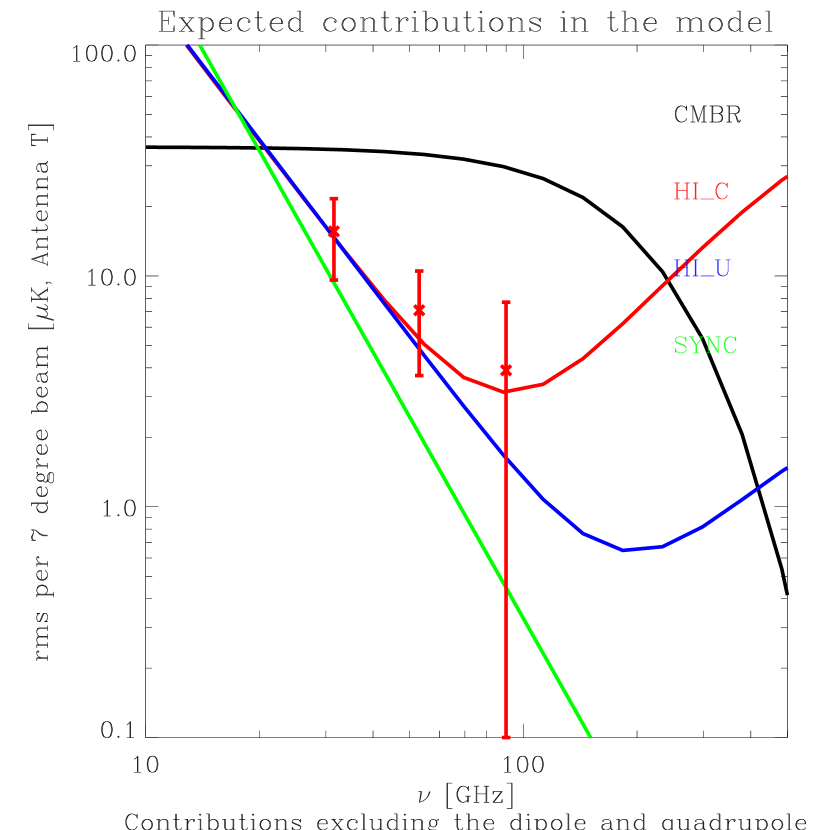
Figure 3: Standard deviation of the fluctuations in the synchrotron, H Icorrelated and uncorrelated emissions in our galactic model, as compared to the CMB fluctuations whose level was set by the DMR measurement, and the data points for the DMR-DIRBE correlated component found by Kogut et al. 95 (see text). A Gaussian beam of 7 degree FWHM was used.

As was shown above, the angular power spectra $C(l)$ of the galactic components all decrease strongly with $\ell$, approximately as $C(\ell)\propto\ell^{-3}$. Smaller angular scales thus bring increasingly small contributions per logarithmic interval of $\ell$ to the variance, $\ell(\ell+1)C(\ell)$: the galactic sky get smoother on smaller angular scales. We set the normalisation constants of the spectra to obtain a level of fluctuations representative of the best half of the sky. In practice, this was achieved by generating an artificial map with $C(\ell)=\ell^{-3}$. We then measured its $\sigma_{T}$ using our previous procedure of measuring the variance in 3 degree patches after convolving with a one degree beam. This gives the required normalisation factor of the power spectra by comparisons with the median values plotted in fig.2.b. We find that

$$\ell\,C_{\ell}^{1/2}=c_{X}\,\ell^{-1/2}\ \mu{\mathrm{K}},$$ (3)

with $c_{X}$ given by $c_{sync}=2.1$, $c_{free}=13.7$, and $c_{dust}=13.5$ at 100 GHz. In addition, one has $c_{HI-U}=8.5$ and $c_{HI-C}=20.6$ for the Dust+Free-free components, uncorrelated and correlated (respectively) with H I.

Of course, by their very construction, these normalisations are only appropriate for intermediate and small scales, about $\ell{\lower 2.15277pt\hbox{$\;\buildrel>\over{\sim}\;$}}10$. The corresponding fluctuation levels at 3.0 mm and 1.4 mm are shown in figure 7. By using these normalisations and our spectral model, we can compute the rms per 7 degree beam at every frequency and check that the H I-correlated component indeed provides a good fit with the results of the Kogut et al. [1996] analysis, as is shown in figure 3.

3 Extragalactic foregrounds

Many detailed studies have been devoted to effects that may blur the primordial signature of the CMB anisotropies. Gravitational lensing by mass concentrations along the light ray paths may for instance alter the detailed map patterns and add a stochastic component. Or photons passing through a fast evolving potential well might be redshifted (Rees-Sciama effect). Secondary fluctuations might be generated during a reionisation phase of the Universe. For all this processes, the answer [Rees and Sciama, 1968, Ostriker and Vishniac, 1986, Seljak, 1996, Jaffe and Kamionkowski, 1998] is that their impact is quite small at scales corresponding to $\ell\simeq 1/\theta{\lower 2.15277pt\hbox{$\;\buildrel<\over{\sim}\;$}}1000$, and can easily be accounted for at the analysis stage of CMB maps. Further fluctuations may also be imprinted, in case of a strongly inhomogeneous reionisation; see e.g.  Aghanim et al. [1996] for further discussion. We shall ignore these effects in the following.

3.1 Infrared and radio sources background

Here we attempt to evaluate what might be the contribution from the Far Infrared Background produced by the line of sight accumulation of extragalactic sources, when seen at the much higher resolution foreseen for future CMB experiments.

Given the steepness of rest-frame galaxy spectra longward of $\sim 100$ $\mu\mathrm{m}$, predictions in this wavelength range are rather sensitive to the assumed high-$z$ history. Indeed, as can be seen from figure 4.a, a starburst galaxy at $z=5$ might be more luminous than its $z=0.5$ counterpart because the redshifting of the spectrum can bring more power at a given observing frequency than the cosmological dimming, at least in the $\lambda{\lower 2.15277pt\hbox{$\;\buildrel>\over{\sim}\;$}}$800 $\mu\mathrm{m}$ range [e.g.   Blain and Longair, 1993] (precisely the range explored by the HFI instrument aboard Planck). This “negative K-correction” means that i) predictions might be relatively sensitive to the redshift history of galaxy formation ii) variations of the observing frequency should imply a partial decorrelation of the galaxy contribution, i.e. one cannot stricto sensu describe this contribution by spatial properties (i.e. a spatial template) and a frequency spectrum (but see below). This is compounded by the fact that this part of the spectrum is not well known observationally, even at $z\simeq 0$, and very little is known about the redshift distribution of faint infrared sources.

Figure 4: Effect of redshifting a template starburst galaxy spectrum (left). Longward of $\sim 300$ $\mu\mathrm{m}$, the flux of such galaxies are similar at all $z{\lower 2.15277pt\hbox{$\;\buildrel>\over{\sim}\;$}}0.5$.

Estimates of the contribution of radio-sources and infrared galaxies to the anisotropies of the microwave sky have till recently relied on extrapolations from redshift $z=0$ all the way to a (large) assumed galaxy formation onset redshift. Given the uncertainties described above, this makes the reliability of the predictions of this type of modelling hard to assess in the $\nu>100$ GHz range. On the other hand, predictions of galaxy formation models in the UV and optical bands have received a lot of attention in the last few years; they rely on substantially more involved semi-analytical models of galaxy formation which provide a physical basis to the redshift history of galaxies [White and Frenk, 1991]. In short, one starts from a matter power spectrum (typically a standard, COBE-normalised CDM), and estimates the number of dark matter halos as a function of their mass at any redshift (e.g.  using the Press-Schechter approach). Standard cooling rates are used to estimate the amount of baryonic material that forms stars. The stellar energy release is obtained from a library of stellar evolutionary tracks and spectra; computations may be then performed to compare in detail with observations. This approach, despite some difficulties, has been rather successful, and many new observations fit naturally in this framework.

This type of physical modelling has recently been extended to the far-infrared range by Guiderdoni et al. [1998]. Given the stellar energy release, Guiderdoni et al. [1998] estimated the fraction reradiated in the microwave range using a simple geometrical model, which yields an infrared luminosity function at all redshifts. This, together with an assignment of synthetic spectra to a given infrared luminosity, allows predictions of the numbers and fluxes of faint galaxies at any frequency. To constrain the fraction of heavily reddened objects as a function of redshift, they used the $z\sim 0$ IRAS data at 60 $\mu\mathrm{m}$ [Lonsdale et al., 1990] to normalise their model, and they further assumed that the isotropic background discovered by Puget et al. [1996] is indeed the long-sought Cosmological Infrared Background (CIBR) due to the accumulated light of infrared sources.

Guiderdoni et al. [1997] selected a small set of possible redshift histories satisfying this (integral) constraint, and predicted that ISO observations at 175 $\mu\mathrm{m}$ could help breaking the remaining degeneracy in the model. Such observations were very recently done [Kawara and al., 1997, Clements et al., 1997, Dole et al., 1999] and the number of sources found is best described by one model of this family (their model E) corresponding to a fairly large fraction of very obscured objects. As shown by figure 5.a, the ISO Hubble deep field data at 15 $\mu\mathrm{m}$ [Oliver et al., 1997] also agree with the predictions of this model. Even the first SCUBA determination [Smail et al., 1997, Blain et al., 1998] at 850 $\mu\mathrm{m}$ seems to be reasonably fitted by model E. In short, this model is successful in predicting the latest source counts over a broad range of frequencies. This gives us confidence that the contribution of infrared galaxies to CMB measurements performed in the same frequency range (that of the HFI, $\nu>100$ GHz) can be assessed with decent accuracy. The situation is different for the redshift distribution of the sources which is more sensitive than the number counts to the details of the evolutionary scenarios. The current observational constraints are so far limited to the spectroscopic follow-up of IRAS sources at 60 $\mu$m which essentially highlights the IR properties of galaxies in the local universe. It is only when redshift follow-up of these new far-infrared catalogs will have been completed that new generations of models can be developed and refined assessment of the infrared source contamination can be made.

In what follows, we shall assume that resolved sources have been removed, and we focus on the spatial and spectral properties of the remaining unresolved background. That can be done only by assuming a specific instrumental configuration giving the level of detector noise and a geometrical beam for each channel. Indeed the variance of the shot noise contributed by $N$ sources of flux $S$ randomly distributed on the sky is $\sigma^{2}=NS$ and the corresponding power spectrum is $C(\ell)=N/(4\pi)S^{2}$. For a population of sources of flux distribution per solid angle $dN/dS/d\Omega$ the power spectrum is, after removing all sources brighter than $S_{c}$

$$C(\ell)=\frac{\sigma_{\rm conf}^{2}}{\Omega_{\rm beam}}=\int_{0}^{S_{c}}\frac{dN}{d\Omega dS}S^{2}dS.$$ (4)

If the cut $S_{c}$ is defined as $S_{c}=q\left(\sigma^{2}_{\rm conf}+\sigma^{2}_{\rm dust}+\sigma^{2}_{\rm instrum}+\sigma^{2}_{\rm CMB}\ldots\right)^{1/2}$ with $q$ fixed to 5, this formula allows to derive iteratively the confusion limit $\sigma_{\rm conf}$. This is the standard deviations of the fluctuations of the unresolved galaxy background, once all sources with $S>5\sigma_{\rm tot}$ (i.e. including the other sources of fluctuations, from cirrus, $\sigma_{\rm dust}$, detector noise $\sigma_{\rm instrum}$, the CMB, $\sigma^{2}_{\rm CMB}$) have been removed.

NUMBER COUNTS WITH Planck HFI
$\nu$	$\theta_{FWHM}$	$\sigma_{ins}$	$\sigma_{cir}$	$\sigma_{CMB}$	$\sigma_{conf}$	$\sigma_{tot}$	$N(>5\,\sigma_{tot})$
GHz	arcmin	mJy	mJy	mJy	mJy	mJy	sr-1
(1)	(2)	(3)	(4)	(5)	(6)	(7)	(8)
857	5	43.3	64	0.1	146	165	954
545	5	43.8	22	3.4	93	105	515
353	5	19.4	5.7	17	45	53	398
217	5.5	11.5	1.7	34	17	40	31
143	8.0	8.3	1.4	57	9.2	58	0.36
100	10.7	8.3	0.8	63	3.8	64	0.17

Table 1: Theoretical estimates from model E of Guiderdoni et al. [1997]. (1) HFI wavebands central frequency in GHz. (2) Beam full width half maximum in arcmin. (3) $1\,\sigma$ instrumental noise for 14 month nominal mission. (4) $1\,\sigma$ fluctuations due to cirrus at $N_{HI}=1.3~{}10^{20}$ cm^-2 (level of the cleanest 10 % of the sky). The fluctuations have been estimated following Gautier et al. (1992) with $P(k)\propto k^{-2.9}$ and $P_{0,100\mu m}=1.4~{}10^{-12}B_{0,100\mu m}^{3}$. (5) $1\,\sigma$ CMB fluctuations for $\Delta T/T=10^{-5}$. (6) $1\,\sigma$ confusion limit due to FIR sources in beam $\Omega\equiv\theta_{FWHM}^{2}$, defined by $\sigma_{conf}=(\int_{0}^{S_{lim}}S^{2}(dN/dS)dS\ \Omega)^{1/2}$. The values $\sigma_{conf}$ and $S_{lim}=q\,\sigma_{tot}$ have been estimated iteratively with $q=5$. (7) $\sigma_{tot}=(\sigma_{ins}^{2}+\sigma_{conf}^{2}+\sigma_{cir}^{2}+\sigma_{CMB}^{2})^{1/2}$. Here $\sigma_{cir}$ is for $N_{HI}=1.3~{}10^{20}$ cm^-2. (8) Surface density of FIR sources for $S_{lim}=5\,\sigma_{tot}$.

Table 1 summarises the E-model results for the HFI instrument Guiderdoni [1998]. The main feature is the very high level of the confusion limit, which translates in modest number of detected sources. One should realize though that this estimate is very pessimistic since it assumes a very naïve source removal scheme by a simple thresholding. In practice one would at least use a compensated filter (e.g. by doing aperture photometry) which removes the contributions to the variance of all long wavelength. A much larger number of sources would then be removed since the counts are very steep (as a matter of example, Guiderdoni et al. [1998] predict with the same model more than 120 000 sources at 350 $\mu$m (860GHz) at flux $>$ 100 mJy, a detection threshold suggested by the recent work of Hobson et al. [1998]). One should thus regard the confusion level derived above as an upper limit which very likely exceeds the real residual unresolved background from sources.

The spectral dependence of the confusion limit can be approximately modelled as that of a modified black body with an emissivity $\propto\nu^{0.70}$ and a temperature of 13.8 K. A more precise fit (at the   20% level) yields at $\nu>$ 100 GHz for the equivalent temperature fluctuation power spectrum (using relative bandwidths of 0.25) is given by

$$\ell C(\ell)^{1/2}\simeq\frac{7.1\ 10^{-9}}{e^{x/2.53}-1}(1-\frac{0.16}{x^{4}})\frac{\sinh^{2}x}{x^{0.3}}\ \ell\ {\rm[K]},$$ (5)

with $x=h\nu/2kT_{0}=\nu/(113.6{\rm GHz})$. This gives a value of $C(\ell)^{1/2}=0.005$  $\mu\mathrm{K}$ at 100GHz. At lower frequencies ($\nu<$ 100 GHz), this model yields instead

$$\ell C(\ell)^{1/2}\simeq 6.3\ 10^{-9}\left(0.8-2.5x+3.38x^{2}\right)\frac{\sinh^{2}x}{x^{4}}\ \ell\ {\rm[K]}$$ (6)

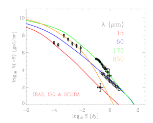
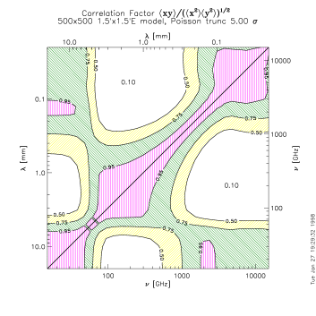
Figure 5: a) Number counts prediction from the E model of Guiderdoni et al. [1997] & the available data (see text). b) Cross-correlation coefficients between maps based on the E model.

Figure 4 shows that the relative fluxes in different observing bands can vary depending on the redshift of the object. Conversely, different bands do not weight equally different redshift intervals. The previous analysis thus does not tell us whether the fluctuation pattern at a given frequency is well correlated with the pattern at another frequency. Of course, the answer will depend on the resolution of the maps and the noise level. To answer this question for the AAO [1998], maps of the galaxy contribution were generated at 30 different frequencies, as in Guiderdoni et al. [1996] and Hivon et al. [1997], but for model E. As shown in figure 5.b, the cross-correlation coefficients of the maps (once the 5$\,\sigma_{tot}$ sources have been removed) is better than 0.95 in the 100-350 GHz range, better than 0.75 in the 350-850GHz, and it is still ${\lower 2.15277pt\hbox{$\;\buildrel>\over{\sim}\;$}}0.60$ in the full 100-1000 GHz range. This indicates that one can treat the IR background from unresolved sources reasonably well as just another template to be extracted from the data, with a fairly well defined spectral behaviour, at least in the range probed by the HFI.

While the model above might well be the best available for bounding the infrared sources properties, it does not take into account the contribution from low-frequency point sources like blazars, radio-sources, etc…which are important at the lower frequencies probed by MAP and the LFI . Using only that model would under-estimate the source contribution at low frequencies. On the other hand, Toffolatti et al. [1998] made detailed predictions in the LFI range which give

$$\ell C(\ell)^{1/2}\simeq\frac{5.7\sinh^{2}(\nu/113.6)}{(\nu/1.5)^{(4.75-0.185\log(\nu/1.5))}}\ \ell\ {\rm[K]}.$$ (7)

This yields $C(\ell)^{1/2}$=0.02  $\mu\mathrm{K}$ at 100GHz. We shall also use that prediction when analysing the expected performances of MAP. Here again, we assume that this unresolved background has well-defined spectral properties.

In order to obtain a pessimistic estimate of the total contribution from sources, we shall consider in the following two uncorrelated backgrounds from sources, the one contributed by IR sources, as described by the equations (5) & (6), and the one contributed by radio-sources, as described by equation(7). The corresponding levels are compared with the other sources of fluctuations in figure 7 and they are quite low (at least at $\ell{\lower 2.15277pt\hbox{$\;\buildrel<\over{\sim}\;$}}1000$) as compared to the expected fluctuations from the CMB or from the Galaxy.

3.2 Clusters of galaxies

Hot ionised gas along the line of sight generate distortions of the CMB fluctuations when the incoming photons scatter off electrons and get a shift in frequency. This translates in an apparent temperature decrement in the low frequency (Rayleigh-Jeans) side of the spectrum, and a temperature excess in the Wien side. This is called the Sunyaev-Zeldovich (hereafter SZ) effect [Zeldovich and Sunyaev, 1969]. The intensity variation of the CMB, $\Delta I_{\nu}/I_{\nu}=y\times f(x)$ is controlled by the Compton parameter

$$y=\frac{k\sigma_{T}}{m_{e}c^{2}}\int T_{e}(l)n_{e}(l)dl,$$ (8)

where $T_{e}$ and $n_{e}$ stand for the electron temperature and density. The spectral form factor in the non relativistic limit depends only on the adimensionnal frequency $x=h\nu/kT_{CMB}$ according to

$$f(x)=\frac{xe^{x}}{(e^{x}-1)}\left[x\left(\frac{e^{x}+1}{e^{x}-1}\right)-4\right].$$ (9)

During the Planck phase A study, Aghanim et al. [1996] devised a model for generating maps of the Sunyaev-Zeldovich effect (both thermal and kinetic) and analysed the capabilities of Planck in detecting clusters of galaxies [Aghanim et al., 1997a, see their Figure 1.6]. Since then, the model was improved by using better estimates of the counts (and of the peculiar velocities), and generalised to encompass various cosmological models. The counts were derived from the Press-Schechter mass function [Press and Schechter, 1974], normalised using the X-ray temperature distribution function derived from Henry and Arnaud [1991] data as in Viana and Liddle [1996]. The following power spectrum of the fluctuations due to the Sunyaev-Zeldovich thermal (hereafter SZ) effect from clusters of galaxies was evaluated by analysing maps of the Compton parameter $y$ generated with these counts.

Figure 6: Power spectra of the Sunyaev-Zeldovich thermal effect for different cosmological models: standard CDM (solid line), open CDM (dashed line) and lambda CDM (dotted line) are shown.

For the standard CDM model, it was found that the $y$ fluctuations spectrum is well-fitted in the range $20<\ell<4000$ by

$$\ell(\ell+1)\,C_{\ell}=a_{ysz}\,\ell\left[1+b_{ysz}\,\ell\right],$$ (10)

with $a_{ysz}=4.3\times 10^{-15}$ and $b_{ysz}=8.4\times 10^{-4}$. Of course, the values of the fitting parameters in equation(10) depend on the assumed cosmological scenario. For an open model ($\Omega_{0}=0.3$), one finds instead $a_{ysz}=4.6\times 10^{-15}$ and $b_{ysz}=2.2\times 10^{-3}$. These are quite small differences, as illustrated by figure 6. This is natural since most of the contributions come from relatively low redshifts while the counts have precisely been normalised via $z\sim 0$ observations. Equation(10) for standard CDM yields

$$\ell\,C_{\ell}^{1/2}=0.27\,\left[\ell\,(1+8.4\times 10^{-4}\,\ell)\right]^{1/2}\,\mu{\mathrm{K}}$$ (11)

for the temperature fluctuation spectrum at 100 GHz.

On small angular scales (large $l$), the power spectrum of the SZ thermal effect exhibits the characteristic dependence of the white noise. This arises because at these scales the dominant signal comes from the point–like unresolved clusters. On large scales (small $l$), the contribution to the power comes from the superposition of a background of unresolved structures and extended structures. The transition between the two regimes occurs for $l\simeq 1/b_{sz}$ that is when the angular scale is close to the pixel size of the simulated maps. One should note though that this approach neglects the effect of the incoherent superposition of lower density ionised regions like filaments. While the contributions in the linear regime are easy to compute [Persi et al., 1995], the non-linear contributions must be evaluated using numerical techniques [Persi et al., 1995, Pogosyan et al., 1996]. While the modelisation above is quite sufficient for the purposes of this paper, detailed simulations of the component separation should benefit from simulated maps of the SZ effect with more realistic low contrast patterns.

The kinetic SZ effect due to the Doppler effect from clusters in motion along the line of sight (hereafter l.o.s) cannot, of course, be spectrally distinguished from the primary fluctuations. This additional contribution is about an order of magnitude smaller than the thermal SZ effect [Aghanim et al., 1997a, b]. We shall thus neglect this contribution to the temperature fluctuations in the following analysis.

4 Comparing contributions to the microwave sky

4.1 Description of the detectors noise

In the course of the measuring process, detector noise is added to the total signal after the sky fluctuations have been observed, which can be described by a convolution with the beam pattern. In order to directly compare the astrophysical fluctuations with those coming from the detectors, it is convenient to derive a fictitious noise field “on the sky” which, once convolved with the beam pattern and pixelised, will be equivalent to the real one Knox [1995]. Modelling the angular response of channel $i$, $w_{i}(\theta)$, as a Gaussian of FWHM $\theta_{i}$, and assuming a white noise detector noise power spectrum, the sky or “unsmoothed” noise spectrum is then simply the ratio of the constant white noise level by the square of the spherical harmonic transform of the beam profile

$$C_{i}(\ell)=c_{noise}^{2}\exp\left(-{(\ell+\frac{1}{2})^{2}\over 2(\ell_{i}+\frac{1}{2})^{2}}\right)\simeq c_{noise}^{2}\exp(-{\ell^{2}\theta_{i}^{2}\over 2\sqrt{2\ln 2}}),$$ (12)

with

$$(\ell_{i}+\frac{1}{2})^{-1}=2\sin\left({\theta_{i}\over 2\sqrt{8\ln 2}}\right)$$

and $c_{noise}^{2}=\sigma_{i}^{2}\Omega_{i}=\sigma_{i}^{2}\times 2\pi[1-\cos(\theta_{i}/2)]$, if $\sigma_{i}$ stands for the 1–$\sigma$ $\Delta T/T$ sensitivity per field of view. The values of $c_{noise}$ for different experiments of interest can be found in Table 2.

While convenient, the noise description above is quite oversimplified. Indeed detector noise is neither white, nor isotropic. The level of the noise depends in particular on the total integration time per sky pixel, which is unlikely to be evenly distributed for realistic observing strategies. In addition, below a (technology-dependent) “knee” frequency, the white noise part of the detector spectrum becomes dominated by a steeper component (typically in $1/f$, if the frequency $f$ is the Fourier conjugate of time). This extra power at long wavelength will typically translate in “stripping” of the noise maps, a common disease. Of course, redundancies can be used to lessen this problem (Wright [1996]), or even reduce it to negligible levels if the knee frequency is small enough [Janssen and al., 1996, Delabrouille, 1998].

MAP (as of January 1998)						BoloBall
$\nu$	22	30	40	60	90	143	217.	353	-	-
$\theta_{FWHM}$	55.8	40.8	28.2	21.0	12.6	8.0	5.5	5	-	-
$\Delta T$	8.4	14.1	17.2	30.0	50.0	35	78	193	-	-
$c_{noise}$	8.8	10.8	9.1	11.8	11.8	11.3	17.4	39.0	-	-

	Proposed LFI				Proposed HFI
$\nu$	30	44	70	100	100	143	217.	353	545	857
$\theta_{FWHM}$	33	23	14	10	10.7	8.0	5.5	5.0	5.0	5.0
$\Delta T$	4.0	7.0	10.0	12.0	4.6	5.5	11.7	39.3	401	18182
$c_{noise}$	2.5	3.0	2.6	2.3	0.9	0.8	1.2	3.7	38	1711

Table 2: Summary of experimental characteristics used for comparing experiments. Central band frequencies, $\nu$, are in Gigahertz, the FWHM angular sizes, $\theta_{FWHM}$, are in arcminute, and $\Delta T$ sensitivities are in $\mu\mathrm{K}$ per $\theta_{FWHM}\times\theta_{FWHM}$ square pixels; the implied noise spectrum normalisation $c_{noise}=\Delta T(\Omega_{FWHM})^{1/2}$, is expressed in $\mu\mathrm{K.deg}$.

4.2 Angular Scale Dependence of the Fluctuations

Figure 7 compares at 30, 100, 217 and 857 GHz the power spectrum of the expected primary anisotropies (in a standard CDM model) with the power contributed by the galactic emission (eq. [3]), the unresolved background of radio and infrared sources (eq. [5, 6, 7]), the S-Z contribution from clusters (eq. [10]), and on-sky noise levels (eq. [12]) corresponding to the Planck mission. It is interesting to note that even at 100 GHz, the dust contribution might be stronger than the one coming from the synchrotron emission, at least for levels typical of the best half of the sky. Since point processes have flat (“white noise”) spectra, their logarithmic contribution to the variance, $\ell(\ell+1)C(\ell)\propto\ell^{2}$, increases and becomes dominant at very small scales.

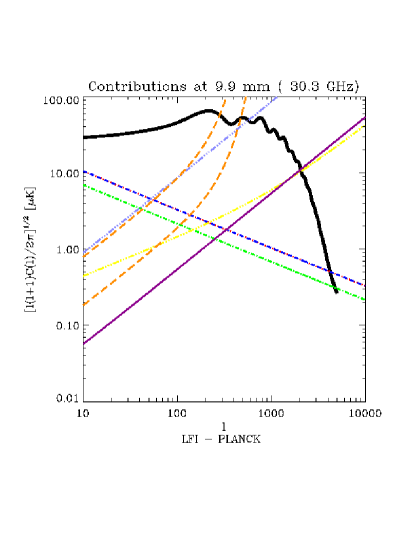
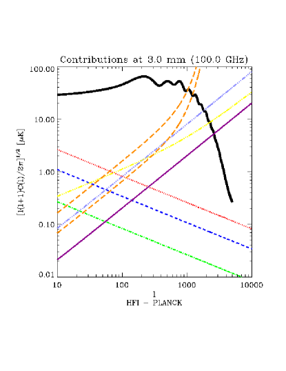
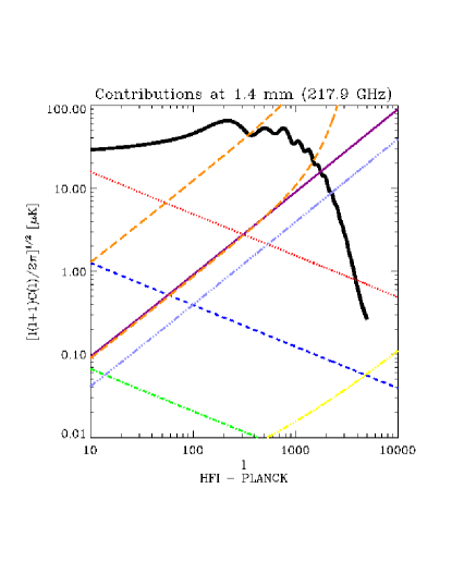
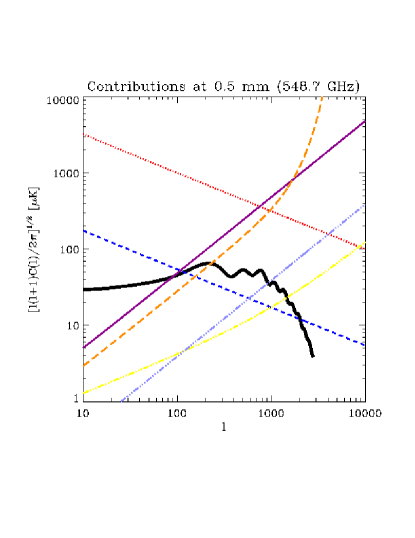
Figure 7: Contributions to the fluctuations of the various components, as a function of angular scale, at different frequencies. The thick solid black line corresponds to the CMB fluctuations of a COBE-normalised CDM model. The dots, dashes and dot-dashes (in red, blue, and green) refer respectively to the HI correlated, HI uncorrelated, and synchrotron emissions of the galaxy. The light blue triple dots-dashes displays the contributions from unresolved radio sources, while the purple line corresponds to the unresolved contribution from infrared sources. Long dashes show “on-sky” noise level (see text, eq. (12)). On the 30 GHz plot, the highest noise level corresponds to MAP, and the lower one to the LFI. On the 100 GHz plot, the highest noise level corresponds to the LFI, and the lower one to the HFI. In the two remaining plots, the noise level corresponds to the HFI case.

4.3 Frequency Scale Dependence of the Fluctuations

Given the power and frequency spectra of the microwave sky model, one can then compare the rms contributions per beam at any frequency $\nu_{i}$ for any experiment by

$$\sigma(\nu_{i})=\sum_{\ell}(2\ell+1)\ C_{\ell}(\nu_{i})\ w_{i}(\ell)^{2},$$ (13)

where $w_{i}$ stands for the transform of the beam profile at the frequency $\nu_{i}$. Figure 8 gives an example for the Planck case.

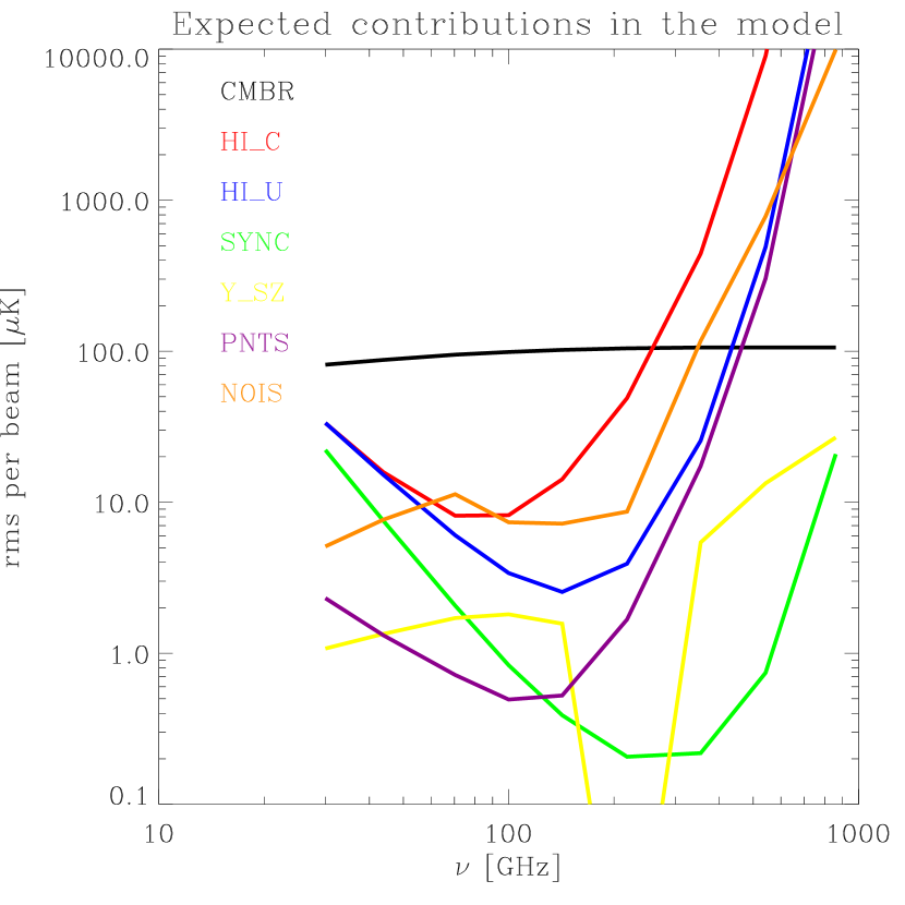
Figure 8: Standard deviation per beam versus frequency for all the relevant model components in the Planck case.

4.4 Angular-Frequency Dependence of the Fluctuations

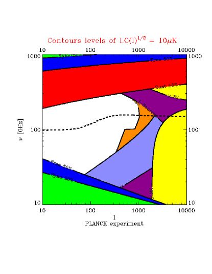
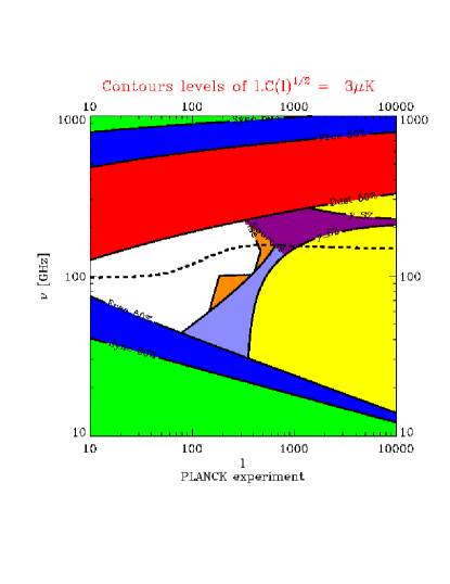
Figure 9: Contour levels of the different components of our model in the angular scale–frequency plane. The levels indicate when the power spectra of the various components reach $(10\mu$K)² and $(3\mu$K)² - respectively one tenth and one hundredth of the level of the COBE detection; the filled side of the lines shows where the corresponding process is higher than the level line (with the same colour coding than in previous plots, but for the HI correlated and uncorrelated components which have been replaced here by the total dust and free-free emissions). Thus the central area is the region where a CMB signal at 1/10 or 1/100 of the COBE level will dominate over all other components. The central dashed line materialises the locus of weakest overall contamination by foregrounds. As before the galactic components corresponds to the median sky level. The noise level shown is for Planck.

An extensive series of angular power spectra at many frequencies (such as those in figure 7), or of amplitudes of fluctuations as a function of frequency for a series of angular scales (such as figure 2), provides a detailed picture of the behaviour of the various components. Still, it is also illuminating to retain the full dependence of the fluctuation amplitudes on frequency and angular scale to build a more synthetic view of the fluctuations “landscape”.

Figure 9 shows the contours in the $\nu-\ell$ plane where the fluctuations, as estimated from $\ell(\ell+1)C(\ell)/2\pi$, reach one tenth (left) or one hundredth (right) of the large scale COBE level [$\ell(\ell+1)C(\ell)/2\pi=(30\mu\mathrm{K})^{2}/10\sim(10\mu\mathrm{K})^{2}$]. These contours map the three dimensional topography of the fluctuations of individual components in the $\nu-\ell$ plane. The synchrotron component (when expressed in equivalent temperature fluctuations) defines a valley which opens towards large $\ell$, since $\ell^{2}C(\ell)$ decreases with $\ell$ as $1/\ell$. The H I-uncorrelated component defines a shallower and gentler valley (see also fig.2.b), while the H I-correlated emission creates a high frequency cliff. The large $\ell$ end of the valley is barred by the point sources “dam”. In any case, even in the case of Planck, the noise level is higher than the contribution from the unresolved sources background.

The heavy black line shows the path followed by a stream lying at the bottom of the valley, i.e. it traces the lowest level of total fluctuations (but noise). Its location confirms that $\nu\simeq 100\,$GHz is the best frequency for low-$\ell$ measurements. At $\ell{\lower 2.15277pt\hbox{$\;\buildrel>\over{\sim}\;$}}200$, the optimal frequency moves to higher values and is determined by the minimum of the fluctuations from unresolved sources and clusters; indeed, the dotted line shows the minimum location if clusters’ fluctuations are ignored. Taking them into account shows that the optimal frequency is ${\lower 2.15277pt\hbox{$\;\buildrel<\over{\sim}\;$}}200$ GHz for high resolution work around $\ell\sim 1000$, rather close to the zero of the Sunyaev-Zeldovich effect at 217 GHz. Of course the exact optimal value depends on the relative weight of the unresolved backgrounds from sources and that from clusters, and cannot be very precise at this stage. Still, the optimal range is $\simeq 150-200$ GHz, which is within the range accessible to the most sensitive detectors available today (typically bolometers can span the 100 to 1000 GHz range). In the case of Planck, one can expect that the most stringent constraints on the high-$\ell$ part of the CMB spectrum will come from the 143 & 217 GHz channel, not the lower frequency ones of lower angular resolution.

Figures available with full version at
$ftp://ftp.iap.fr/pub/from\_users/bouchet/wiener7.ps.gz$

Figure 10: Each hatched areas delimits the regions where a given component accounts for 50% of the total contribution to the variance including noise, in a particular experiment. Each panel has been restricted to the frequency range that the experiment span. Inner contours show when a component accounts for 90% of the signal, and the central contour (horizontal hatches) delimits the region where the CMB anisotropies should contribute 99% of the signal. a) on the left is shown the MAP case. b) the right panel corresponds to Planck.

In order to better identify the dominant contributions in a given experiment, Figure 10 shows the regions of the $\nu-\ell$ plane where the contribution from a given process $\ell\,C_{p}(\ell)$ accounts for half of the total including the noise, $\ell\,\sum_{p}C_{p}(\ell)$ (i.e. of the contribution per logarithmic interval centred around that scale $\ell$ to the variance of the measurement at frequency $\nu$). The inner contours show when that process accounts for 90% of the total (and 99% for the CMB). This figure thus shows the areas in the $\nu$-$\ell$ plane where a given component will be dominating the measurements.

Two cases were considered for illustration. On the left, the noise level and the frequency range correspond to the MAP experiment which uses passively cooled HEMT detectors, while the Planck case which combines actively cooled HEMTs and bolometers is shown on the right. In the latter case, reaching 10% accuracy on the CMB anisotropies over all modes between a few and a thousand, in the cleanest 50% of the sky, should be easily accessible. A 1% accuracy can only be obtained though in a substantially smaller angular range, if no foreground subtraction is performed. We now turn to that issue.

5 Separation of components

Our goal in this section is to introduce a simple tool, which we denote as the “quality factor” of an experiment, that will allow in §6 a comparison of experimental set-ups, once the effect of foregrounds is included. We start by establishing notations for describing our model of the sky (§5.1) and derive in §5.2 a formulation of the separation problem. General properties of linear inversion methods are described in §5.3. The Wiener filtering method is described in §5.4, and §5.5 gives the properties of this method, while §5.6 shows that a simple indicator allows capturing most aspects of the inversion. Simple examples and more technical points are discussed in the final sub-section.

5.1 Physical model

We note $\mathcal{F}(\nu,\mathbf{e})$ the flux at a frequency $\nu$ in the direction on the sphere referenced by the unit vector $\mathbf{e}$. We make the hypothesis that $\mathcal{F}(\nu,\mathbf{e})$ is a linear superposition of the contributions from $N_{c}$ components, each of which can be factorised as a spatial template $\mathcal{T}_{p}(\mathbf{e})$ at a reference frequency (e.g. at 100 GHz), times a spectral coefficient $g_{p}(\nu)$

$$\mathcal{F}(\nu,\mathbf{e})=\sum_{p=1}^{N_{c}}g_{p}(\nu)\,\mathcal{T}_{p}(\mathbf{e}).$$ (14)

This factorisation is not stricto sensu applicable to the background due to unresolved point sources, since at different frequencies different redshift ranges dominate, and thus different sources. But even at the Planck-HFI resolution, this is, as we showed earlier, a weak effect which can be safely ignored for our present purposes.

Let us also note that the factorisation assumption above does not restrict the analysis to components with a spatially constant spectral behaviour. Indeed, these variations are expected to be small, and can thus be linearised too. For instance, in the case of a varying spectral index whose contribution can be modelled as $\nu^{\alpha(\mathbf{e})}\mathcal{T}_{p}(\mathbf{e})$, we would decompose it as $\nu^{\overline{\alpha}}[1+(\alpha(\mathbf{e})-\overline{\alpha})\ln\nu]\mathcal{T}_{p}(\mathbf{e})$. We would thus have two spatial templates to recover, $\mathcal{T}_{p}(\mathbf{e})$ and $(\alpha(\mathbf{e})-\overline{\alpha})\mathcal{T}_{p}(\mathbf{e})$ with different spectral behaviours, $\propto\nu^{\overline{\alpha}}$ and $\propto\nu^{\overline{\alpha}}\ln\nu$ respectively. But given the low expected level of the high latitude synchrotron emission, this is unlikely to be necessary. This simple trick may still be of some use though to describe complex dust properties in regions with larger optical depth than assumed here (see also the alternative way proposed by Tegmark [1998]).

5.2 The separation problem

During an experiment, the microwave sky is scanned by arrays of detectors sensitive to various frequencies and with various optical responses and noise properties. Their response is transformed in many ways by the ensuing electronics chains, by interactions between components of the experiments, the transmission to the ground, etc. The resulting sets of time-ordered data (TOD) needs then to be heavily massaged to produce well-calibrated pixelised maps at a number of frequencies, each with an effective resolution, and well specified noise properties. We assumed here that all this work has already been done (for further details, see Janssen and Gulkis [1992], Wright [1996], Tegmark [1997], Delabrouille [1998], Delabrouille et al. [1998]).

We thus focus on the next step, i.e. the joint analysis of noisy pixelised sky maps, or signal maps $\mathbf{s}_{i}$, at $N_{\nu}$ different frequencies in order to extract information on the different underlying physical components. It is convenient to represent a pixelised map as a vector containing the $N_{p}$ map pixels values, the $j$-th pixel corresponding to the direction on the sky $\mathbf{e}_{j}$. Let us denote by $\mathbf{t}_{p}$ the unknown pixelised maps of the physical templates $\mathcal{T}_{p}$. We thus have to find the best estimates of the templates $t_{p}(\mathbf{e}_{j})$, which are related to the observed signal by the $N_{\nu}\times N_{p}$ equations

$$s_{i}(\mathbf{e}_{j}) = \sum_{p=1}^{N_{c}}\ \int_{\nu=0}^{\infty}d\nu\ v_{i}(\nu-\nu_{i})\,g_{p}(\nu)\sum_{k=1}^{N_{p}}w_{i}(\mathbf{e}_{j}-\mathbf{e}_{k})\ t_{p}(\mathbf{e}_{k})+n_{i}(\mathbf{e}_{j})$$ (15)

$$= \sum_{p=1}^{N_{c}}\left[v_{i}\star g_{p}(\nu)\right]\,\left[w_{i}\star t_{p}(\mathbf{e})\right]+n_{i}(\mathbf{e}_{j}),$$ (16)

where $\star$ stands for the convolution operation. This system is to be solved assuming we know for each signal map its effective spectral and optical transmission, $v_{i}(\nu-\nu_{i})$ and $w_{i}(\mathbf{e})$ and that the covariance matrix $\mathbf{N}_{i}=\left\langle\mathbf{n}_{i}\mathbf{n}_{i}^{T}\right\rangle$ of the (unknown) noise component $\mathbf{n}_{i}$ has been properly estimated during the first round of analysis.

Since the searched for templates $\mathbf{t}_{p}$ are convolved with the beam responses, $w_{i}$, it is in fact more convenient to formulate the problem in terms of spherical harmonics transforms (denoted by an over-brace), in which case the convolutions reduce to products. For each mode $\boldsymbol{\ell}\equiv\{\ell,m\}$, we can arrange the data concerning the $N_{\nu}$ channels as a complex vector of observations, $\mathbf{y}(\boldsymbol{\ell})\equiv\{\overbrace{s_{1}}(\boldsymbol{\ell}),\overbrace{s_{2}}(\boldsymbol{\ell}),\ldots,\overbrace{s_{N_{\nu}}}(\boldsymbol{\ell})\}$, and we define similarly a complex noise vector, $\mathbf{b}(\boldsymbol{\ell})\equiv\{\overbrace{n_{1}}(\boldsymbol{\ell}),\overbrace{n_{2}}(\boldsymbol{\ell}),\ldots,\overbrace{n_{N_{\nu}}}(\boldsymbol{\ell})\}$, while the corresponding template data will be arranged in a complex vector $\mathbf{x}(\boldsymbol{\ell})$ of length $N_{c}$. We thus have to solve for $\mathbf{x}$, for each mode $\boldsymbol{\ell}$ independently, the matrix equation

$$\mathbf{y}(\boldsymbol{\ell})=\mathbf{A}(\boldsymbol{\ell})\mathbf{x}(\boldsymbol{\ell})+\mathbf{b}(\boldsymbol{\ell}),$$ (17)

with $A_{ip}(\boldsymbol{\ell})=\left[v_{i}\star g_{p}(\nu)\right]\,w_{i}(\boldsymbol{\ell})$. Note though the independence of the $\boldsymbol{\ell}$ modes would be lost in case one uses other functions that spherical harmonics (e.g. to insure orthogonality of the basis functions when all the sky is not available for the analysis [Gorski, 1994]). Then instead of solving $N_{p}$ systems of $N_{\nu}$ equations, one will have to tract a much larger system of $N_{p}\times N_{\nu}$ equations (possibly in real space rather than in the transformed space). For simplicity we treat each mode separately in the following.

5.3 Linear Inversions

Any linear recovery procedure may be written as an $N_{c}\times N_{\nu}$ matrix $\mathbf{W}(\ell)$ which applied to the $\mathbf{y}(\boldsymbol{\ell})$ vector yields an estimate $\widehat{\mathbf{x}}(\boldsymbol{\ell})$ of the $\mathbf{x}(\boldsymbol{\ell})$ vector, i.e.

$$\widehat{\mathbf{x}}(\boldsymbol{\ell})=\mathbf{W}(\boldsymbol{\ell})\,\mathbf{y}(\boldsymbol{\ell}).$$ (18)

In the following, we show that the matrix $\mathbf{R}=\mathbf{W}\mathbf{A}$ plays in important role in determining the properties of the estimated templates by the selected method, whatever it might be. Indeed, since $\widehat{\mathbf{x}}=\mathbf{W}\left[\mathbf{A}\mathbf{x}+\mathbf{b}\right]$, we have

$$\left\langle\widehat{\mathbf{x}}\right\rangle=\mathbf{R}\left\langle\mathbf{x}\right\rangle\quad\mathrm{and}\quad\left\langle\widehat{\mathbf{x}}\widehat{\mathbf{x}}^{\dagger}\right\rangle=\mathbf{R}\left\langle\mathbf{x}\mathbf{x}^{\dagger}\right\rangle\mathbf{R}^{\dagger}+\mathbf{W}\mathbf{B}\mathbf{W}^{\dagger},$$ (19)

where $\mathbf{x}^{\dagger}$ is the Hermitian conjugate of $\mathbf{x}$ (i.e. $\mathbf{x}^{\dagger}$ is the complex conjugate of the transpose, $x^{T}$, of the vector $\mathbf{x}$), and $B=\left\langle\mathbf{b}\mathbf{b}^{\dagger}\right\rangle$ stands for the (supposedly known) noise covariance matrix. We denote by $\left\langle Y\right\rangle$ the average over an ensemble of statistical realisations of the quantity $Y$. The covariance matrix of the reconstruction errors, $\mathbf{E}$, is given by

$$\mathbf{E}\equiv\left\langle(\mathbf{x}-\widehat{\mathbf{x}})(\mathbf{x}-\widehat{\mathbf{x}})^{\dagger}\right\rangle=\mathbf{C}-\mathbf{R}\mathbf{C}-\mathbf{C}\mathbf{R}^{\dagger}+\left\langle\widehat{\mathbf{x}}\widehat{\mathbf{x}}^{\dagger}\right\rangle,$$ (20)

where $\mathbf{C}=\left\langle\mathbf{x}\mathbf{x}^{\dagger}\right\rangle$ stands for the covariance matrix of the underlying templates.

An estimate of this covariance matrix $\mathbf{C}$ should of course be estimated from the data itself. Since the elements of the covariance matrix of the recovered templates (assuming they have zero mean) may be written as

$$\left\langle\widehat{x}_{p}\widehat{x}_{q}^{\star}\right\rangle=R_{pp}\left\langle x_{p}x_{q}^{\star}\right\rangle R_{qq}^{\star}+\sum_{r\neq p}\sum_{s\neq q}R_{pr}\left\langle x_{r}x_{s}^{\star}\right\rangle R_{sq}^{\dagger}+\left[\mathbf{W}\mathbf{B}\mathbf{W}^{\dagger}\right]_{pq},$$ (21)

we define the intermediate variable $\widetilde{x}_{p}=\widehat{x}_{p}/R_{pp}$ in order to write

$$\left\langle\widetilde{x}_{p}\widetilde{x}_{q}^{\star}\right\rangle=\left\langle x_{p}x_{q}^{\star}\right\rangle+\mathcal{B},$$ (22)

where $\mathcal{B}$ is then an additive bias. This shows that an unbiased estimate of the covariance matrix of the unknown templates, $\widehat{\mathbf{C}}$, may be obtained by

$$\widehat{\mathbf{C}}\equiv\widehat{\left\langle\mathbf{x}\mathbf{x}^{\dagger}\right\rangle}={1\over 2\ell+1}\sum_{m=-\ell}^{m=+\ell}\widetilde{\mathbf{x}}\widetilde{\mathbf{x}}^{\dagger}-\mathcal{B}.$$ (23)

This expression is only formal though, since $\mathcal{B}$ contains some of the unknowns. Still, this form allows to generalise the calculation of Knox [1995] of the expected error (covariance) of the power spectra estimates derived in such a way from the maps. Indeed,

$$\mathrm{Cov}\left[\widehat{C}_{pq}\right] = \left\langle\widehat{C}_{pq}^{2}\right\rangle-\left\langle\widehat{C}_{pq}\right\rangle^{2}$$ (24)

$$= \left\langle\left[{1\over 2\ell+1}\sum_{m}\widetilde{x}_{p}\widetilde{x}_{q}^{\star}-\mathcal{B}_{pq}\right]^{2}\right\rangle-C_{pq}^{2}.$$ (25)

Once this expression is developed, there are many terms with fourth moments of the form $\left\langle x_{r}(\ell,m)\,x_{s}(\ell,m)^{\star}\,x_{t}(\ell,m^{\prime})\,x_{u}(\ell,m^{\prime})\right\rangle$.

If we assume that all the $x_{p}$ are Gaussian variables, then we can express these fourth moments as products of second moments, and recontract the sums to finally obtain

$$\mathrm{Cov}\left[\widehat{C}_{pq}\right] = (\widehat{C}_{pq}+\mathcal{B}_{pq})^{2}+{2\over 2\ell+1}(\widehat{C}_{pq}+\mathcal{B}_{pq})^{2}$$ (26)

$$- 2\mathcal{B}_{pq}((\widehat{C}_{pq}+\mathcal{B}_{pq})+\mathcal{B}_{pq}^{2}-\mathbf{C}_{pq}^{2}$$ (27)

$$= {2\over 2\ell+1}(C_{pq}+\mathcal{B}_{pq})^{2}={2\over 2\ell+1}\left\langle{\widehat{x}_{p}\over R_{pp}}{\widehat{x}_{q}^{\star}\over R_{qq}^{\star}}\right\rangle^{2}.$$ (28)

This expression shows the extra contribution of noise and foregrounds to the cosmic variance. It can be re-expressed and simplified once a specific inversion method has been specified.

5.4 Wiener filtering

One particular choice of $\mathbf{W}$ may be obtained by minimising the figure of merit

$$\chi^{2}(\boldsymbol{\ell})=(\mathbf{y}-\mathbf{A}\widehat{\mathbf{x}})^{\dagger}\ \mathbf{B}^{-1}\ (\mathbf{y}-\mathbf{A}\widehat{\mathbf{x}}),$$ (29)

for each mode $\boldsymbol{\ell}$. The advantage of this simple inversion by $\chi^{2}$ minimisation is that it requires no prior information on the unknown $\mathbf{x}$, only some knowledge on the statistical properties of the noise maps through their covariance matrix $\mathbf{B}$. An assessment of this simple method will be given in a sequel paper (hereafter paper II) concerned with actual numerical simulations of the sky and its analysis.

Another possibility for linearly separating the components is to apply “Wiener” filtering techniques since Bouchet et al. [1996b] and Tegmark and Efstathiou [1996] showed how to generalise this well-known procedure (see e.g. Bunn et al. [1994], Bond [1995] for an application to COBE-DMR data, and Zaroubi et al. [1995] for galaxy surveys data) to the case of multi-frequency, multi-resolution, data. In the following, we rederive in a self-contained way this Wiener filtering approach, with a number of extensions which will prove useful for our purposes.

The inversion by $\chi^{2}$ minimisation is designed to best reproduce the observed data set by minimising the residuals between the observations and the model (eq. [29]). Another possibility is to require a statistically minimal error in the recovery, when the method is applied to an ensemble of data sets with identical statistical properties. One then obtains the “Wiener” matrix $\mathbf{W}$, by demanding that the vector of differences between the underlying and recovered templates, $\boldsymbol{\varepsilon}=\mathbf{x}-\widehat{\mathbf{x}}$, be on average of minimal norm

$$\varepsilon^{2}(\boldsymbol{\ell})=\left\langle|\mathbf{x}-\widehat{\mathbf{x}}|^{2}\right\rangle\equiv\left\langle(\mathbf{x}-\widehat{\mathbf{x}})^{\dagger}(\mathbf{x}-\widehat{\mathbf{x}})\right\rangle$$ (30)

In practice, we require that the derivatives of

$$\varepsilon^{2}(\boldsymbol{\ell}) = \left\langle|\mathbf{x}-\mathbf{W}(\mathbf{A}\mathbf{x}+\mathbf{b})|^{2}\right\rangle$$ (31)

$$= (W_{p\nu}A_{\nu p^{\prime}}-\delta_{pp^{\prime}})(W_{p\nu^{\prime}}A_{\nu^{\prime}p^{\prime\prime}}-\delta_{pp^{\prime\prime}})\left\langle x_{p^{\prime}}x_{p^{\prime\prime}}^{\star}\right\rangle+W_{p\nu}W_{p\nu^{\prime}}\left\langle b_{\nu}b_{\nu^{\prime}}^{\star}\right\rangle$$ (32)

versus all $W_{p\nu}$ (and their complex conjugate) be zero for each $\ell$ (with repeating indices implying summation in(32) and (33)), which yields

$$W_{p\nu}\left[A_{\nu p^{\prime}}\left\langle x_{p^{\prime}}x_{p^{\prime\prime}}^{\star}\right\rangle A_{\nu^{\prime}p^{\prime\prime}}+\left\langle b_{\nu}b_{\nu^{\prime}}^{\star}\right\rangle\right]=A_{\nu^{\prime}p^{\prime}}\left\langle x_{p^{\prime}}x_{p}^{\star}\right\rangle.$$ (33)

In matrix form, the wiener matrix is then given by

$$\mathbf{W}=\mathbf{C}\mathbf{A}^{T}\left[\mathbf{A}\mathbf{C}\mathbf{A}^{T}+\mathbf{B}\right]^{-1},$$ (34)

if we denote by $\mathbf{C}$ the covariance matrix of the templates, $C_{pp^{\prime}}=\left\langle x_{p}x_{p^{\prime}}^{\star}\right\rangle$. Alternatively, $\mathbf{W}^{\dagger}=\left[\mathbf{A}\mathbf{C}\mathbf{A}^{T}+\mathbf{B}\right]^{-1}\mathbf{A}\mathbf{C}\$ (since $\mathbf{A}$ is real, $\mathbf{A}^{\dagger}=\mathbf{A}^{T}$).

Since the Wiener matrix depends on $\mathbf{C}$, i.e. on the covariance matrix of the templates, it is clear that this makes use of prior knowledge to construct optimal weights. One can thus think of Wiener filtering as a “polishing” stage of a first inversion (e.g. as in § 5.3) yielding an estimate $\widehat{\mathbf{C}}$ of the covariance matrix needed to have optimal weights. A practical implementation is described in paper II.

5.5 Characteristics of the Wiener Separation

The definition (33) of Wiener filtering implies that

$$\left\langle\widehat{\mathbf{x}}\mathbf{x}^{\dagger}\right\rangle=\left\langle\mathbf{x}\widehat{\mathbf{x}}^{\dagger}\right\rangle=\left\langle\widehat{\mathbf{x}}\widehat{\mathbf{x}}^{\dagger}\right\rangle.$$ (35)

As a result, the expression for the covariance matrix of the reconstruction errors $\mathbf{E}\equiv\left\langle\boldsymbol{\varepsilon}\boldsymbol{\varepsilon}^{\dagger}\right\rangle$ reduces to the simple form

$$\mathbf{E}=\left[\mathbf{I}-\mathbf{R}\right]\mathbf{C},$$ (36)

where $\mathbf{I}$ stands for the identity matrix, and $\mathbf{R}=\mathbf{W}\mathbf{A}$ as before. Alternatively, $\mathbf{E}=\mathbf{C}\left[\mathbf{I}-\mathbf{R}^{\dagger}\right]$.

The general expression of the covariance matrix of the templates given by eq. (19) may be simplified by using the specific Wiener matrix properties of eqs. (35) and (36), which yields

$$\left\langle\widehat{\mathbf{x}}\widehat{\mathbf{x}}^{\dagger}\right\rangle=\mathbf{R}\left\langle\mathbf{x}\mathbf{x}^{\dagger}\right\rangle.$$ (37)

Both equations(36) and(37) clearly show that the closer $\mathbf{R}$ is to the identity, the smaller are the reconstruction errors.

The diagonal elements of $\mathbf{E}$ are of particular interest since they give the residual errors on each recovered template,

$$\varepsilon_{p}^{2}=E_{pp}=(1-R_{pp})C_{pp}.$$ (38)

To break down this overall error into its various contributions, we start from eq. (32)

$$\varepsilon_{p}^{2}=(1-R_{pp})^{2}C_{pp}+\sum_{p^{\prime}\neq p\neq p^{\prime\prime}}R_{pp^{\prime}}R_{pp^{\prime\prime}}C_{p^{\prime}p^{\prime\prime}}+W_{p\nu}W_{p\nu^{\prime}}B_{\nu\nu^{\prime}}.$$ (39)

By using eq. (38), we get

$$\varepsilon_{p}^{2}={1\over R_{pp}}\sum_{p^{\prime}\neq p\neq p^{\prime\prime}}R_{pp^{\prime}}R_{pp^{\prime\prime}}C_{p^{\prime}p^{\prime\prime}}+W_{p\nu}W_{p\nu^{\prime}}B_{\nu\nu^{\prime}},$$ (40)

which describes the power leakage from the other processes and the co-added noises.

In addition, the error on the deduced power spectra given by eq. (28) takes for Wiener filtering the simple form

$$\mathrm{Cov}\left[\widehat{C}_{pq}\right]\equiv\left[\Delta\widehat{C}_{pq}\right]^{2}={2\over 2\ell+1}\left[{R_{pr}C_{rq}\over R_{pp}R_{qq}^{\star}}\right]^{2},$$ (41)

which will prove particularly convenient to compare experiments.

5.6 Case of uncorrelated templates

In this theoretical analysis, we can always assume for simplicity that we have decomposed the sky flux into a superposition of emissions from uncorrelated templates, so that

$$\left\langle x_{p}x_{p^{\prime}}^{\star}\right\rangle=\delta_{pp^{\prime}}\,C_{pp}(\ell)=\delta_{pp^{\prime}}\,\mathcal{C}_{p}(\ell).$$ (42)

In our galactic model, it means in particular that we consider the templates for the H I-correlated and H I-uncorrelated components rather than those for the dust and free-free emissions. In actual implementations though it might prove more convenient to relax this assumption and consider correlated templates but with simpler spectral signatures (see Paper II). In the uncorrelated case, the previous expressions (37, 38 & 40, 41) may be written as

$$\left\langle|\widehat{x}_{p}|^{2}\right\rangle = Q_{p}\left\langle|x_{p}|^{2}\right\rangle=Q_{p}\mathcal{C}_{p}(\ell)$$ (43)

$$\varepsilon_{p}^{2} = (1-Q_{p})\mathcal{C}_{p}=1/Q_{p}\sum_{p^{\prime}\neq p}R_{pp^{\prime}}^{2}\mathcal{C}_{p^{\prime}}+W_{p\nu}W_{p\nu^{\prime}}B_{\nu\nu^{\prime}}$$ (44)

$$\Delta\widehat{\mathcal{C}}_{p} = \sqrt{{2\over 2\ell+1}}{\mathcal{C}_{p}\over Q_{p}}$$ (45)

where $Q_{p}=\mathbf{R}_{pp}$ stands for the trace elements of $\mathbf{W}\mathbf{A}$. Thus $Q_{p}$ tells us

1. how the typical amplitude of the Wiener-estimated modes $\widehat{\mathbf{x}}$ are damped as compared to the real ones (eq. [43]).

2. the spectrum of the residual reconstruction error in every map (eq. [44]); note that this error may be further broken down in residuals from each component in every map by using the full $\mathbf{R}$ matrix.

3. the uncertainty added by the noise and the foreground removal ($\propto 1/Q_{p}-1$, eq. [45]) to cosmic (or sampling) variance which is given by $C_{pp}/\sqrt{2\ell+1}$ (this result only holds though under the simplifying assumption of Gaussianity of all the sky components).

Given these interesting properties, we propose to use $Q_{p}$ as a “quality factor” to assess the ability of experimental set-ups to recover a given process $p$ in the presence of other components; it assesses in particular how well the CMB itself can be disentangled from the foregrounds.

Section 6 below is devoted to “practical” uses of the quality factor, in conjunction with our assumed sky model.

5.7 Discussion

5.7.1 Simple examples

This “quality” indicator generalises the real space “Foreground Degradation Factor” introduced by Dodelson and Stebbins [1994]. It may be viewed as an extension of the usual window functions used to describe an experimental setup. This can be seen most easily by considering a noiseless thought experiment mapping directly the CMB anisotropies with a symmetrical beam profile $w(\theta)$. Then the power spectrum of the map will be the real power spectrum times the square of the spherical harmonic transform of the beam, $<\widehat{x}_{p}(\ell)>=w(\ell)^{2}<x_{p}(\ell)>$. The spherical transform of $Q_{p}^{1/2}(\ell)$ is then the beam profile of a thought experiment directly measuring CMB anisotropies. The shape of $Q_{p}(\ell)$ thus gives us a direct insight on the real angular resolution of an experiment when foregrounds are taken into account.

In addition, one often considers (e.g. for theoretical studies of the accuracy of parameter estimation from power spectra) a somewhat less idealised experiment which still maps directly the CMB, with a beam profile $w(\theta)$, but including also detector noise, characterised by its power spectrum $C_{N}$. Let us suppose this is analysed by Wiener filtering. We have to solve $\mathbf{y}=\mathbf{A}x+\mathbf{n}$, with

$$A^{T}=\{w,w,w,w,\ldots\},\quad\left\langle xx^{\dagger}\right\rangle=C_{x},\quad\mathbf{B}=C_{N}\times\boldsymbol{I}.$$ (46)

The previous formulae then lead to

$$Q_{x}(\ell) = {C_{x}(\ell)\over C_{x}(\ell)+w^{-2}C_{N}(\ell)/N_{c}}$$ (47)

$$\Delta\widehat{C}_{x} = {2\over 2\ell+1}{C_{x}(\ell)\over Q_{x}}={2\over 2\ell+1}\left(C_{x}(\ell)+w(\ell)^{-2}\,C_{N}(\ell)/N_{c}\right),$$ (48)

where $N_{c}$ stands as before for the number of channels (measurements). Equation(47) tells us that the Wiener-estimated modes (as seen by the ratio of the estimated to real spectra) are damped by the ratio of the expected signal to signal + noise (the noise power spectrum being “on the sky”, cf.  §4.1, with the noise power spectrum being the noise power spectrum per channel divided by the number of channels). In brief, what Wiener filtering does when the noise strength is getting larger than the signal is to progressively set the estimate of the signal to zero in an attempt to return only true features. And of course we recover the traditional error on the estimated power spectrum added by noise found by Knox [1995]. Thus determining the quality factor allows to find the equivalent ideal experiment often considered by theorists; it provides a direct estimate of the final errors on the power spectrum determination from a foreground model and the summary table of performance of an experiment.

5.7.2 Reduced variables

Note that the expressions found previously could be further simplified by considering reduced templates, $\mathbf{x}^{\prime}$ which are uncorrelated and of unit variance. Indeed, let us perform a Cholesky decomposition of $\mathbf{C}$, i.e. $\mathbf{C}=\mathbf{L}\mathbf{L}^{T}$ where $\mathbf{L}$ is a lower triangular (real) matrix. The reduced templates are then defined by $\mathbf{x}^{\prime}=\mathbf{L}^{-1}\mathbf{x}=\mathbf{L}^{T}\mathbf{C}^{-1}\mathbf{x}$ (which implies, as desired that the reduced templates are “orthonormalised”, $\left\langle\mathbf{x}^{\prime}\mathbf{x}^{\prime\dagger}\right\rangle=\mathbf{L}^{T}\mathbf{C}^{-1}\left\langle\mathbf{x}\mathbf{x}^{\dagger}\right\rangle\mathbf{C}^{-1\,T}\mathbf{L}=\mathbf{I}$).

Then the problem to solve may be written as

$$\mathbf{y}=\mathbf{S}\mathbf{x}^{\prime}+\mathbf{b},$$ (49)

where we have defined $\mathbf{S}=\mathbf{A}\mathbf{L}$. Since $\left\langle\mathbf{y}\mathbf{y}^{T}\right\rangle=\mathbf{S}\mathbf{S}^{T}+\mathbf{B}$, $\mathbf{S}\mathbf{S}^{T}$ is the useful signal covariance matrix (and $\mathbf{S}$ may be seen as it’s Cholesky decomposition). In that case,

$$\mathbf{W}^{\prime} = \mathbf{S}^{\dagger}\left[\mathbf{S}\mathbf{S}^{\dagger}+\mathbf{B}\right]^{-1}$$ (50)

$$\mathbf{E}^{\prime} = \left\langle(\mathbf{x}^{\prime}-\widehat{\mathbf{x}}^{\prime})(\mathbf{x}^{\prime}-\widehat{\mathbf{x}}^{\prime})^{\dagger}\right\rangle=\mathbf{I}-\mathbf{R}^{\prime}$$ (51)

$$\mathbf{R}^{\prime} = \mathbf{L}^{-1}\mathbf{R}\mathbf{L}=\mathbf{S}^{\dagger}\left[\mathbf{S}\mathbf{S}^{\dagger}+\mathbf{B}\right]^{-1}\mathbf{S}.$$ (52)

This form shows most clearly that the Wiener filter derived is indeed a generalisation of the usual signal to noise weighting (eq. (52)). On the other hand, this convenient form for theoretical analysis might not be so practical since $\mathbf{C}$ might be rather ill-determined from a first step of analysis. Thus paper II will rather use the formulae obtained in the previous sections.

6 Comparing experimental set-ups

6.1 Examples of Wiener matrixes

Once the instrument, through the $\mathbf{A}$ matrix, and the covariance matrix $\mathbf{C}$ of the templates are known, the Wiener filter is entirely determined through equation (34). Figure 11 offers a graphical presentation of the resulting values of the Wiener matrix coefficients of the CMB component when we use our sky model (assuming negligible errors in designing the filter). It shows how the different frequency channels are weighted at different angular scales and thus how the $\nu-\ell$ information gathered by the experiment is used.

In the MAP case, most weight is given to the 90 GHz channel. It is the only one to gather CMB information at $\ell{\lower 2.15277pt\hbox{$\;\buildrel>\over{\sim}\;$}}600$, and it’s own weight becomes negligible at $\ell{\lower 2.15277pt\hbox{$\;\buildrel>\over{\sim}\;$}}1000$. In the LFI case, the main CMB channel is the 100 GHz one, which gathers information till $\ell\sim 1500$, while the 70 GHz channel is of some help till $\ell\sim 1100$. The two other channels only contribute at $\ell{\lower 2.15277pt\hbox{$\;\buildrel<\over{\sim}\;$}}500$. The situation is different in the HFI case, since no single channel dominates at all scales. The 143 GHz channel is dominant till $\ell\sim 1400$ and useful till $\ell\sim 2000$, while the 217 GHz channel becomes dominant at $\ell{\lower 2.15277pt\hbox{$\;\buildrel>\over{\sim}\;$}}1400$ and gather CMB information till $\ell\sim 2300$. The 100 GHz channel contribution to the CMB determination is only modest, and peaks at $\ell\sim 800$.

Once the information from the LFI and the HFI are considered jointly, the previous HFI weights are barely affected, and the LFI weights appear to be sizeable only in the 100 GHz channel, albeit at a fairly reduced level as compared to the 100 GHz channel of the HFI (which is itself only a modest contributor to the CMB determination). As a result, this already suggests that the impact of the LFI on the high $\ell$ HFI measurements ($\ell>200$) will be in controlling systematics and possibly in better determining the foregrounds. Of course, one should note that this analysis assumes the foregrounds are known well enough to design the optimal filter. Thus the LFI impact might be greater in a more realistic analysis when the filter is designed with the only help of the measurements themselves.

Figure 11: CMB Wiener matrix elements at $\ell>200$ for MAP, the LFI, the HFI and the full Planck mission. Each bin in $\ell$ is the average over one hundred contiguous values. The frequency bins are centred at the average frequency of each channel, but their width in not representative of their spectral width.

6.2 Effective windows and beams

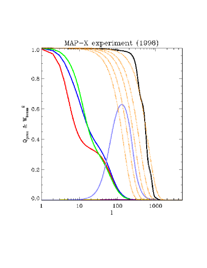
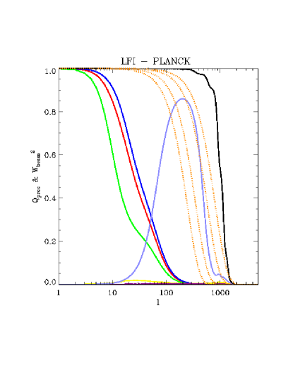
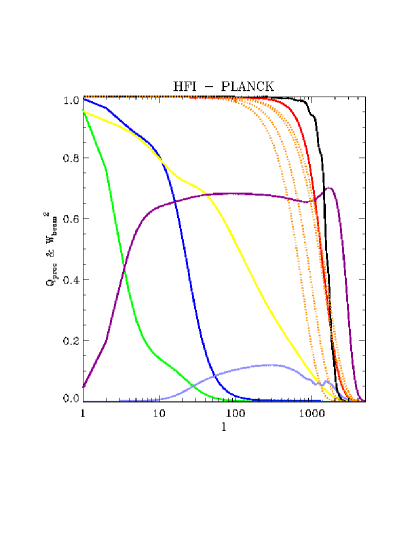
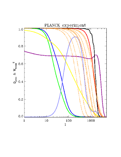
Figure 12: Square of the $\ell$-space effective windows (i.e. $Q_{p}$) for the LFI, HFI, and PlanckȦs usual, black is for the CMB, red, blue, and green are for the Galactic components, yellow is for the SZ contribution. The transform of the channel optical beams are shown for comparison as dotted orange lines.

Figure 12 gives the effective $\ell$-space window of the experiment for each component, $Q_{p}(\ell)$, to be compared with the individual windows of each channel, $w_{i}(\ell)$. For the CMB, it shows the gain obtained by combining channels through Wiener filtering. For MAP, the effective beam is nearly equal to it’s 90 GHz beam, while the improved noise level of the LFI allows it to do much better than it’s “best” beam would suggest (in particular at $\ell\sim 1000$). None of these two experiments can separate the SZ or the infrared sources background contribution. As expected the Galactic foregrounds are poorly recovered except on the largest scales (small $\ell$) where their signal is strongest (we assumed spectra $\propto\ell^{-3}$). The only exception is that of the H I-correlated component which is of course very well traced by the HFI. When the LFI and the HFI are combined, the main improvement appears to be on the SZ contribution thanks to the greater spectral level arm offered to distinguish it from other foregrounds.

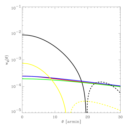
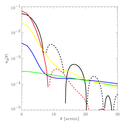
Figure 13: Corresponding real space effective beams (negative parts are denoted by dashes). As usual, black is for the CMB, red, blue, and green are for the Galactic components, yellow is for the SZ contribution.

Figure 13 shows the inverse spherical harmonics transforms of the $Q_{p}(\ell)$, i.e.  the effective angular beams. They show the effective point spread function by which the underlying maps of the component emissions would have been convolved once the analysis is complete. One can see in particular that the FWHM of the CMB beam is $\simeq 16.5^{\prime}$ for MAP and $\simeq 7.5^{\prime}$ for Planck (and even better for the dust components).

6.3 Maps reconstruction errors

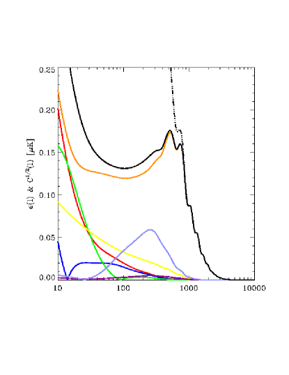
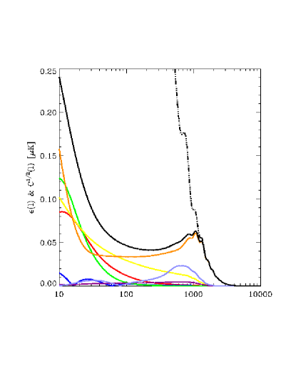
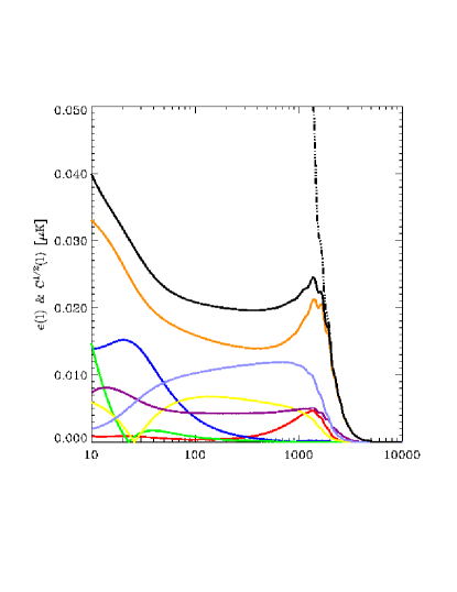
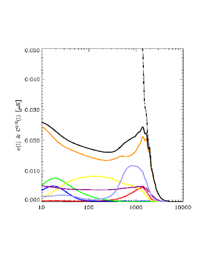
Figure 14: CMB reconstruction error contributed by each component (with the same line coding than above) and their total in black. The integral of $\ell(\ell+1)\varepsilon^{2}/2\pi$ would give the reconstruction error of the map. The dashed-dotted line shows for comparison $C(\ell)^{1/2}$ for the CMB. For Planck, the total of the reconstruction error is nearly constant at all $\ell$ and corresponds to $\varepsilon(\ell){\lower 2.15277pt\hbox{$\;\buildrel<\over{\sim}\;$}}0.025$  $\mu\mathrm{K}$, a factor greater than six below the MAP case.

We now estimate the spectrum of the reconstruction errors in the map. Figure 14 compares these residual errors per individual $\boldsymbol{\ell}$ mode with the typical amplitude of the true signal. The first thing to note is that the error spectrum cannot be accurately modelled as a simple scale-independent white noise (as expected from the $\nu-\ell$ shape of the Wiener matrix for the CMB) . We also see that the LFI improves on MAP mostly by decreasing the noise contribution, but at the largest scales where the galactic contributions are also lowered. The LFI taken jointly with the HFI helps in reducing the low-$\ell$ galactic emissions, and the power leakage from the radio-sources background. The contributions per logarithmic bin of $\ell$ to the variance are compared in figure 15. It is interesting to note that in the Planck case the largest contribution but noise comes from SZ clusters in the range $50{\lower 2.15277pt\hbox{$\;\buildrel>\over{\sim}\;$}}\ell{\lower 2.15277pt\hbox{$\;\buildrel>\over{\sim}\;$}}500$, to be then superseded by the leakage from the radio-sources background.

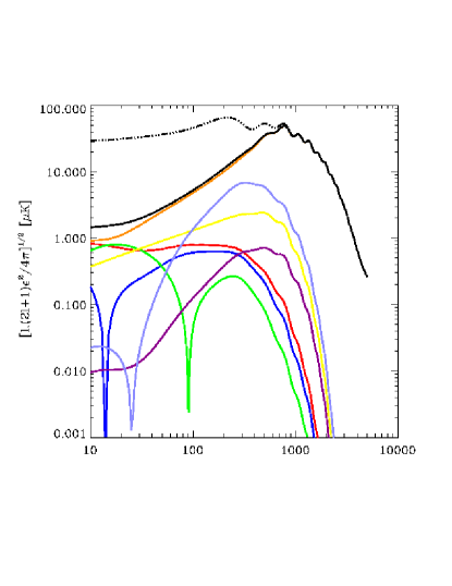
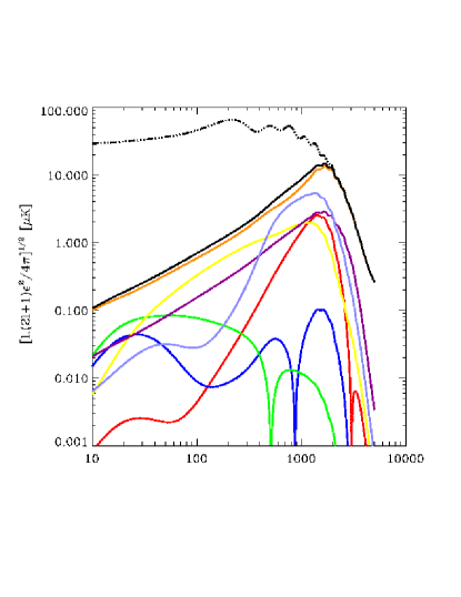
Figure 15: CMB reconstruction errors compared with the input spectrum in the MAP (left) and Planck case (right).

6.4 Foreground and noise induced errors on the CMB power spectrum

Finally, we can estimate the uncertainty added by the noise and foreground removal to the CMB power spectrum. Figure 16 shows the envelope of the 1-$\sigma$ error expected from the the current design of MAP(green), the LFI (blue), and the HFI or the full Planck (red), as well as a “boloBall” experiment meant to show what bolometers on balloon might achieve soon; the experimental characteristics used in this comparison may be found in table 2. Note that there has been no “band averaging” in this plot, which means that there is still cosmological signal to be extracted from the HFI at $\ell\sim 2500$. The message from this plot is thus excellent news since it tells us that even accounting for foregrounds, Planck will be able to probe the very weak tail of the power spectrum and allow breaking the near degeneracy between some of the cosmological parameters.

The second panel of the figure shows the variations induced by changing the target CMB theory. In this case, a flat universe with a (normalised) cosmological constant of 0.7 was assumed. What MAP can say on the third peak would then be much reduced, while on the contrary the HFI would probe accurately one more peak. This illustrates the fact that the errors on the signal will of course depend on the amplitude of the signal; it is a reminder of the fact that the numbers given so far are meant to be illustrative. As already stressed, the merit of this approach is to offer a quantitative tool for comparisons. The impact of changing the foreground model will be addressed in section §6.7.

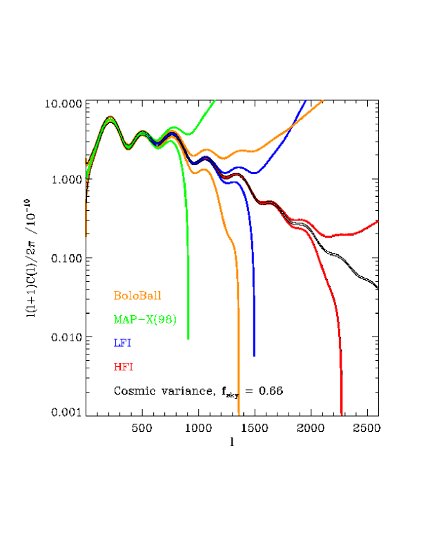
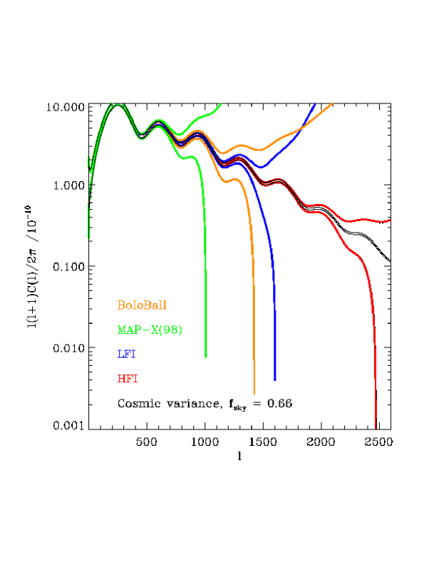
Figure 16: Expected errors on the amplitudes of each mode individually (no band averaging) for different experiments (the full Planck is indistinguishable from the HFI case). The thin central lines gives the target theory plus or minus the cosmic variance, for a coverage of 2/3 of the sky. a) Standard CDM b) Lambda CDM (with $\Omega_{b}=0.05,\ \Omega_{CDM}=0.25,\ \Omega_{\Lambda}=0.7,\ h=0.5$).

6.5 Wiener versus “naïve” error estimates:

In the previous section we estimated the error bars reachable on the CMB power spectrum assuming a sky model and a separation method. In effect we found an equivalent ideal experiment described by an “on-sky” noise power spectrum $[w^{-2}C_{N}]_{eff}=C_{CMB}[1/Q_{CMB}-1]$. Numerous papers have been devoted to estimating the possible accuracy of determinations of the cosmological parameters from CMB experiments. To forecast this accuracy, various recipes were used to derive an estimate of this effective on-sky noise spectrum from tables of performance of the experiment such as table 2. One option has been to assume that all frequency channels but one are used to remove the foregrounds contribution from the “best” CMB channel, i.e. the one closest to 100 GHz, or the most sensitive one. A less radical proposition by Bond et al. [1997] has been to assume that all channels but $N_{keep}$ are used to clean the $N_{keep}$ closest to 100 GHz, which are then assumed to contain only the CMB signal and noise, with an effective “on-sky” power spectrum of this noise $[w^{-2}C_{N}]_{eff}$ given by

$${1\over[w^{-2}C_{N}]_{eff}}=\sum_{i=1}^{N_{keep}}{1\over w_{i}^{-2}C_{N,i}},.$$ (53)

This is a generalisation of the formula (47) to unequal noise power spectra, $C_{N,i}$ in different channels. This approach does not tell how many and which $N_{keep}$ channels can be considered clean once the $N_{c}-N_{keep}$ others have been somehow used for foreground removal.

Figure 17 compares the fractional error $\Delta C_{CMB}/C_{CMB}$ expected from Wiener filtering and different prescriptions, namely using the best channel or all channels in some frequency range combined according to equation (53). As expected we see that the error in the “naïve” estimates of the uncertainty of the CMB power spectrum goes to zero at small $\ell$, when cosmic variance dominates over the noise, and at large $\ell$ when detector noise dominates all foreground contributions. If only the best channel (dashes) of the experiment is retained (i.e. $\nu=90,143$ GHz respectively for MAP & Planck), the error is of course always over estimated, i.e. optimal use of all channels by Wiener filtering does much better than this naïve estimator would suggest.

The error in estimating the noise level is much decreased if the channels between 55 and 300 GHz (i.e. the 60 & 90 GHz channels of MAP and the 70, 100, 143 and 217 GHZ channels of Planck) are retained in the sum (53). A better estimate for MAP obtains if one also includes the 40 GHz channel, since one now underestimates the error by only the few per cent over the full $\ell$ range. For Planck on the contrary retaining all channels between 55 and 300 GHz already underestimates the errors by 10 % at $\ell\sim 1500$. Assuming that all Planck channels between 35 and 400 GHz can be cleaned with the help of the remaining ones further increases the error on the CMB uncertainty to more than 15 % at $\ell\sim 1800$.

More importantly, this error is scale-dependent, i.e. it shows that no “naïve” prescription gives a fair estimate of the CMB power spectrum uncertainties at all scales. This is not surprising, given the shapes of the Wiener matrixes we saw in figure 11. These shapes indeed illustrate that an optimal estimate of the CMB component obtains by weighting differently as a function of scale the informations coming from different channels, according to their angular resolution, and to the levels of their detector noise and of their foregrounds contaminations.

The results above show that the relative error between Wiener based and other error estimates of the CMB spectrum are relatively small, but they are scale dependent, and the same naïve prescription might either underestimate or overestimate the errors depending on the experiment considered. This invites exercising some restraint in using results based on these simple prescriptions, like the usual comparison of accuracy of cosmological parameters determinations by different experiments. Of course, our Wiener based estimates cure only some of the limitations of standard analyses since many simplifying (and unrealistic) assumptions remain. The main limitations of course arises from the idealised description of the measurement process (eq. (17)) and the assumed perfect knowledge of the response matrix, $\mathbf{A}$, and the correlation matrix, $\mathbf{C}$.

Figure 17: Ratio versus scale of naïve error estimates of the CMB power spectrum to the one derived from the quality factor. This ratio is given both for MAP (left) and the full Planck (right).

6.6 Experiment optimisation and robustness

One may wonder whether the CMB residuals will vary linearly with global variations of the noise figures of an experiment, as could be produced for instance by variations of the operating temperature, or length of operation of the experiment (allowing different number of sky coverages), or simply overly optimistic or pessimistic estimates of the detectors performances. Figure 18 shows the variation of the rms of the total residual contribution from noise and unsubtracted foregrounds to a CMB map as a function of the noise level compared to the nominal one. The square of this rms value is obtained by integrating the residual spectrum of figure 14 till a maximum $\ell_{max}$. Varying $\ell_{max}$ gives a concise description of the contribution of various scales to the map error.

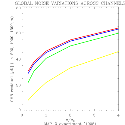
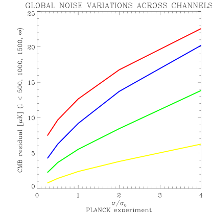
Figure 18: Performance variations for global variations across channels of the detector noise level (e.g. with the number of sky coverages done). The yellow, green, and blue lines correspond to restricting the integration to a maximum $\ell_{max}$ of respectively $500,1000,1500$. The red line corresponds to no restriction at all.

In the nominal case, $\sigma/\sigma_{0}=1$, one sees that for MAP and Planck respectively the residuals are 21 and 2.5 $\mu\mathrm{K}$ for “low”-resolution maps retaining only the modes till $\ell_{max}=500$. For medium resolution maps with $\ell\leq 1000$, these errors increase to 41 and 5.5 $\mu\mathrm{K}$, and high-resolution maps with $\ell\leq 1500$ have residuals of 50 and 9 $\mu\mathrm{K}$ respectively. If all $\ell$ are retained, the rms of the residual are then 52 and 13 $\mu\mathrm{K}$. The difference between MAP and Planck in the increase of the residual with the number of modes retained reflects the difference in angular resolution of the maps produced by Wiener filtering (figures 12 and 13).

For “low” and medium resolution maps, the residuals for Planck vary nearly linearly with the noise level. This is the high-$\ell$ part which is most affected by variations of the noise level. In the MAP case, the stronger curvature of the lines indicate that it would be more affected by sub-nominal performance of the detectors, and conversely that it would benefit more of an increase of the mission duration; a decrease of the noise level by a factor of two (e.g. 4 years instead of one year of operation) would for instance reduce the residuals for $\ell<1000$ from 41 to $\sim$ 30 $\mu\mathrm{K}$.

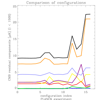
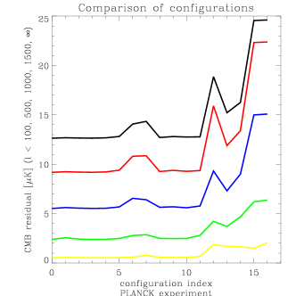
Figure 19: a) CMB residuals (in a map with all modes till $\ell_{max}=1500$) retained) in various configurations for Planck. The black curve displays the total, and the other lines detail the various contributions from noise (orange curve) and foregrounds with the same colour coding than figures 7 or 8 (i.e. red, blue, and green curves correspond to the Galactic residuals, yellow is for the thermal SZ, and the light blue and purple curves are for the unresolved sources backgrounds). b) Total residual in different configurations, for different $\ell_{max}$ (as in figure 18, the yellow, green, and blue lines correspond to restricting the integration to a maximum $\ell_{max}$ of respectively $500,1000,1500$, while the red line corresponds to no restriction at all). c) Table of configuration indexes in the adjacent figures.

The quality factor approach may also be used to test whether the failure of a single channel of an experiment would be critical for the outcome of the experiment, i.e. whether it is robust. Here we estimate the variation of the CMB residuals in different “crippled” configurations for Planck. Figure 19 shows that i) the residuals are dominated by noise ii) there is nearly no impact at all if a single Planck channel is lost except for the 143 & 217 GHz channels iii) loosing the HFI would more than double the residuals, but the LFI completed by the HFI 217 or 353 GHz channel would already do rather well.

6.7 Uncertainties of the sky model

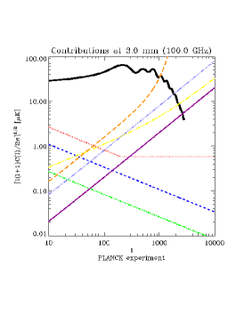
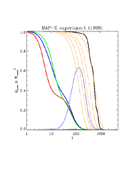
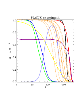
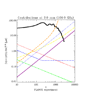
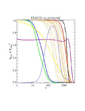
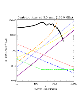
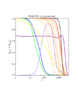
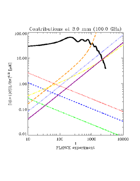
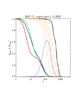
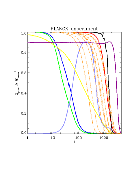
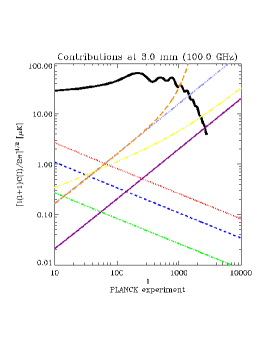
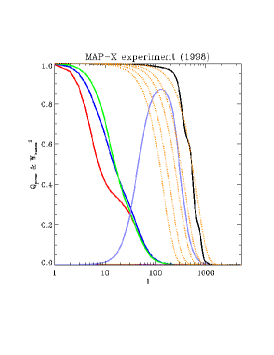
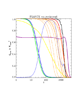
Figure 20: Power spectra at 100 GHz (including HFI noise, left column) and corresponding quality factors for MAP and Planck (respectively middle and right column) for various variations of the sky model. The colour coding of the various foregrounds is the same than in similar previous figures. In the top row, the spectrum of H I-correlated component flattens to $\ell{-2}$ at $\ell>200$, while this flattening is rather for the H I-uncorrelated component (second row) and the synchrotron emission (third row). The last two rows corresponds to higher levels of the backgrounds from unresolved infrared sources (fourth row) or radio-sources.

Figure 16 illustrated the fact that the deduced 1-$\sigma$ errors on the CMB spectrum depend on the amplitude of that signal by comparing the results for a standard and a “Lambda-CDM” model. Given the observed variations one may worry that all the results obtained so far might critically depend on the details of the sky model assumed. This is potentially frightening since clearly the situation regarding foregrounds emission might be quite more complicated than assumed here (e.g. some free-free may locally be emitted at higher temperature, the backgrounds from unresolved sources might be higher, etc).

We have thus considered variations on the basic sky model used so far. For the three galactic components, we considered cases when each power spectrum might level off and become $\propto\ell^{-2}$ at $\ell>200$, resulting in an increase of power by a factor of 10 at $\ell=2000$ as compared to our basic assumption of a constant slope of -3 at all scales. We also considered that the level of the free-free like emission uncorrelated with the HI-emission might be four times lower. We also increased independently the normalisation of each unresolved foreground component by a factor of four. We allowed each of these 6 variation to occur in combination with all the others, thereby creating 64 different foreground models.

Figure 20 shows the resulting 100 GHz power spectra in 5 of these 64 configurations, as well as the corresponding quality factors for MAP and Planck. As anticipated, the effective transmission of a foreground component is improved when and where the amplitude of that component is increased. But the transmission of the other components does not appear affected. This is not really surprising either, since Wiener filtering is a signal to (signal+noise) weighting, where (signal+ noise) obtains for the contribution from detectors noise and of of all the astrophysical components. The lack of sensitivity of the transmission of all components but the one varied simply reflects the fact that the dominant terms are the CMB and detector noise, which are precisely those which were kept untouched here.

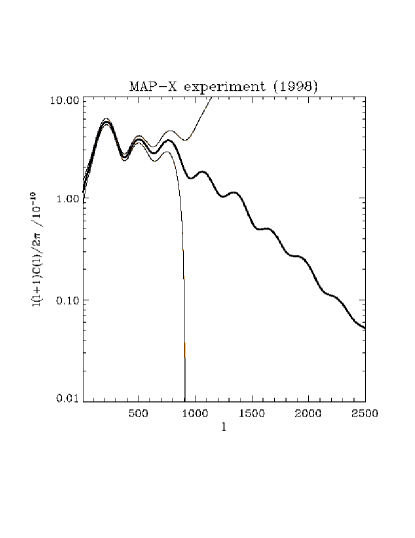
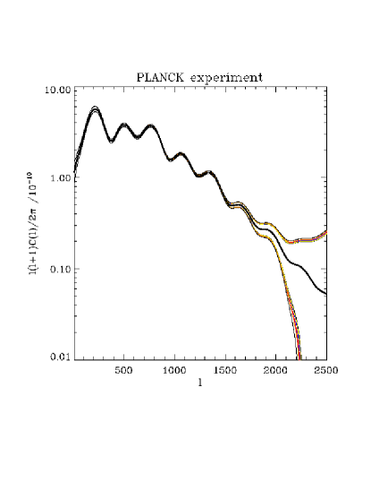
Figure 21: Effect of variations in the sky model (see text) on the deduced $1-\sigma$ error area for the CMB power spectrum. Both in the MAP (left) and Planck (right) case, the 64 variations investigated barely affect the result because the dominant contributions to the signal in the channels of most weight for the CMB determination are the CMB itself and the detector noise.

Figure 21 displays the extent of $1-\sigma$ error for the CMB power spectrum in the case of MAP and Planck for the 64 sky models explored. Nearly all curves are superimposed, which demonstrates that the deduced errors are rather robust to variations in the details of the sky model. This is simply because the dominant contributions to the signal in the channel of most weight for the CMB determination remained the CMB itself and the detector noise. Thus if the main features of the sky model proposed here are correct, it is unlikely that most results obtained in this paper will be much modified.

7 Conclusions

In order to assess the expected level of foreground contamination to be expected in CMB experiments we have developed a simple sky model based on current knowledge. In this model, the microwave emission of the sky is the superposition of the CMB, three galactic emission mechanism, in addition to two unresolved backgrounds from sources, one associated with radio-sources and the uncorrelated other one arising from infrared sources. Further fluctuations are imprinted by the Sunyaev-Zeldovich effect of clusters. While not known precisely, we believe that the non-CMB components are reasonably well constrained by current data supplemented with modest theoretical extrapolations.

We then analysed aspects of the data analysis of multi-frequency multi-resolution observations. Wiener filtering is shown to allow building optimal linear estimates of the spatial templates of the physical processes, as defined by their spectral behaviour. We computed specific examples of Wiener filters for our sky model and several experimental set-up. The shape of the CMB Wiener filter in the $\nu-\ell$ space allows to build intuition on how the information from different frequency channels is combined at different angular scales to minimise the residuals in a CMB map. We further showed as a function of scale the fraction of residuals which arise from detector noise and from partly unsubtracted foregrounds. Integrating these residuals show for instance that the rms reconstruction error from modes $\ell<1000$ should be $\sim 40$  $\mu\mathrm{K}$ for MAP and smaller than 6 $\mu\mathrm{K}$ for Planck.

We also introduced a simple measure of the effective resolution of multi-frequency multi-resolution experiments in the presence of foregrounds. It’s harmonic transform is the effective point spread function by which the underlying maps of the component emissions would have been convolved once the analysis is complete. This effective transmission or window function is directly related to the expected uncertainty on the power spectra determinations once foregrounds are accounted for (under the assumption of Gaussian foregrounds though). Typically, MAP will probe well the CMB power spectrum till $\ell\sim 900\ (1000)$ and Planck till $\ell\sim 2300\ (2500)$ for a standard (or a Lambda) CDM model. We find that simpler estimates make a scale-dependent error in estimating the spectrum uncertainty and that depending on the experiment they might yield an over- or an under-estimates.

As further examples of the usefulness of this simple analytical framework, we computed how the rms reconstruction error is affected by global noise level variations in an experiment, as induced for instance by a variation in the mapping duration of the experiment. MAP is relatively sensitive to such variations, while the variation is closer to linear for Planck. We also analysed the robustness of Planck to various failures leading to the loss of some channels. The most important channels are the 143 and 217 GHz, but even their total loss would result in less than a 10 % increase in the residual rms. Loosing all HFI channels but the 217 GHz one would only yield a 20 % increase, but it’s loss would then nearly double the residual rms! Clearly, optimisation trade-off should not result in decreasing the sensitivity of the 217 GHz and neighbouring channels.

Of course, assessing the effect of foregrounds relies to some extent on the realism of the foregrounds model. We considered 64 sky models differing by what appears to be the least well established features. We found that the quality of the CMB recovery should be basically unaffected, mainly because the dominant high-$\ell$ contributions in the channels of most weight for the CMB determination are the CMB itself and detector noise. This excellent news should nevertheless be taken with a grain of salt. Indeed, it was always assumed a nearly optimal filter could be built, which entails some knowledge of the foregrounds (i.e. their very existence, their power spectra, and their frequency dependence). Paper II will address some of these points by means of direct numerical simulations. We can already note though that a strong foreground at least in some channels should be no problem since the needed information will be easily obtained from the data itself. Forgetting a very weak foreground in all channels should not lead to great errors. The difficult case will of course be to make sure that no unsuspected foreground is sizeable mostly in the primary CMB channels.

But much new data is becoming available to improve on our current knowledge of the microwave sky, either from the analysis of data from the ISO satellite, of ongoing $H_{\alpha}$ and radio surveys, and of many ground and balloon experiment. And of course the future generations of CMB satellite themselves were designed to much increase this knowledge by mapping most of the sky in a large frequency range and with much improved noise levels as compared to COBE. The analysis above thus makes us rather confident that foregrounds should not prevent the future CMB satellites from finally unveiling the CMB power spectrum with high accuracy.

References

- AAO [1998] Planck-HFI. C. AAO. High frequency instrument for the planck mission, a proposal to the european space agency. Proposal submitted in response to the Annoucement of Opportunity of ESA, 1998.
- Abergel et al. [1994] A. Abergel, F. Boulanger, A. Mizuno, and Y. Fukui. Comparative analysis of the far-infrared and (13)co (j = 0-1) emissions of the taurus complex. Ap. J. Lett., 423:L59–L62, Mar. 1994.
- Aghanim et al. [1997a] N. Aghanim, A. De Luca, F. R. Bouchet, R. Gispert, and J. L. Puget. Cosmology with sunyaev-zeldovich observations from space. A&A, 325:9–18, Sept. 1997a.
- Aghanim et al. [1996] N. Aghanim, F.-X. Désert, J.-L. Puget, and R. Gispert. Ionization by early quasars and cosmic microwave background anisotropies. A&A, 311:1–11, July 1996.
- Aghanim et al. [1997b] N. Aghanim, S. Prunet, O. Forni, and F. R. Bouchet. The effect of moving lenses on the cmb. submitted to A&A, 1997b.
- Bennett et al. [1994] C. L. Bennett, A. Kogut, G. Hinshaw, A. J. Banday, E. L. Wright, K. M. Górski, D. T. Wilkinson, R. Weiss, G. F. Smoot, S. S. Meyer, J. C. Mather, P. Lubin, K. Loewenstein, C. Lineweaver, P. Keegstra, E. Kaita, P. D. Jackson, and E. S. Cheng. Cosmic temperature fluctuations from two years of cobe differential microwave radiometers observations. Ap. J., 436:423–442, Dec. 1994.
- Bersanelli et al. [1996] M. Bersanelli, F. R. Bouchet, G. Efstathiou, M. Griffin, J.-M. Lamarre, R. Mandolesi, H. Norgaard-Nielsen, O. Pace, J. Polny, J.-L. Puget, J. Tauber, N. Vittorio, and S. Volonte. Phase a report, . http://astro.estec.esa.nl/SA-general/Projects/Planck/report/report.html, 1996.
- Blain et al. [1998] A. W. Blain, J.-P. Kneib, R. J. Ivison, and I. Smail. Deep counts of submillimeter galaxies. astroph/9812412, 1998. to be published in ApJ, 512, L87-L90 (1999).
- Blain and Longair [1993] A. W. Blain and M. S. Longair. Submillimetre cosmology. MNRAS, 264:509+, Sept. 1993.
- Bond [1995] J. R. Bond. Phys. Rev. Lett., 74:4369, 1995.
- Bond et al. [1997] J. R. Bond, G. Efstathiou, and M. Tegmark. Forecasting cosmic parameter errors from microwave background anisotropy experiments. MNRAS, 291:L33–L41, Nov. 1997.
- Bouchet et al. [1997] F. R. Bouchet, F. Gispert, R. Boulanger, and J.-L. Puget. Comparing performances of cmb experiments. In F. R. Bouchet, R. Gispert, B. Guiderdoni, and J. Trân Thanh Vân, editors, “Microwave Background Anisotropies”, Proceedings of the Moriond Astrophysics meeting, held in Les Arcs, France, March 16th-23rd, 1996, pages 481–502. Editions Frontières, 1997.
- Bouchet et al. [1996a] F. R. Bouchet, R. Gispert, and J.-L. Puget. The cobras/samba cmb project. In S. Maurogordato, C. Balkowski, C. Tao, and J. Trân Thanh Vân, editors, Clustering in the Universe; Proceedings of the Moriond meeting, Les Arcs, France, pages 537–544. Editions Frontières, 1996a. astro-ph/9507032.
- Bouchet et al. [1996b] F. R. Bouchet, R. Gispert, and J.-L. Puget. The mm/sub-mm foregrounds and future cmb space missions. In E. Dwek, editor, Unveiling the Cosmic Infrared Background; held in 1995 in College Park, MD; AIP Conference Proceedings 348, Baltimore, Maryland, USA, pages 255–268, 1996b.
- Boulanger et al. [1996] F. Boulanger, A. Abergel, J. P. Bernard, W. B. Burton, F. X. Desert, D. Hartmann, G. Lagache, and J. L. Puget. The dust/gas correlation at high galactic latitude. A&A, 312:256–262, Aug. 1996.
- Bunn et al. [1994] E. F. Bunn, K. B. Fisher, Y. Hoffman, O. Lahav, J. Silk, and S. Zaroubi. Wiener filtering of the cobe differential microwave radiometer data. Ap. J. Lett., 432:L75–L78, Sept. 1994.
- Burton and Hartmann [1994] W. B. Burton and D. Hartmann. The leiden/dwingeloo survey of emission from galactic hi. Astrophys.and Space Sc., 217:189–193, July 1994.
- Clements et al. [1997] D. L. Clements, J.-L. Puget, G. Lagache, W. Reach, R. Gispert, H. Dole, C. Cesarsky, D. Elbaz, H. Aussel, F. Bouchet, B. Guiderdoni, A. Omont, F.-X. Desert, and A. Franceschini. Deep 175 micron counts with iso: A new population? Bull. American Astron. Soc., 191, #63.05, 191:6305+, Dec. 1997.
- Davies et al. [1996a] R. D. Davies, C. M. Gutierrez, J. Hopkins, S. J. Melhuish, R. A. Watson, R. J. Hoyland, R. Rebolo, A. N. Lasenby, and S. Hancock. Studies of cosmic microwave background structure at dec.=+40 deg - i. the performance of the tenerife experiments. MNRAS, 278:883–896, Feb. 1996a.
- Davies et al. [1996b] R. D. Davies, R. A. Watson, and C. M. Gutierrez. Galactic synchrotron emission at high frequencies. MNRAS, 278:925–939, Feb. 1996b.
- De Bernardis et al. [1992] P. De Bernardis, S. Masi, and N. Vittorio. Cmb and galactic maps in the millimetric region. In The infrared and submillimetre sky after COBE; Proceedings of the NATO Advanced Study Institute, Les Houches, France, Mar. 20-30, 1991, pages 315–330, 1992.
- De Oliveira-Costa et al. [1997] A. De Oliveira-Costa, A. Kogut, M. J. Devlin, C. B. Netterfield, L. A. Page, and E. J. Wollack. Galactic microwave emission at degree angular scales. Ap. J. Lett., 482:L17–+, June 1997.
- Delabrouille [1998] J. Delabrouille. Analysis of the accuracy of a destriping method for future cosmic microwave background mapping with the planck surveyor satellite. Astronomy and Astrophysics Supplement Series, 127:555–567, Feb. 1998.
- Delabrouille et al. [1998] J. Delabrouille, K. M. Gorski, and E. Hivon. Circular scans for cosmic microwave background anisotropy observation and analysis. MNRAS, 298:445–450, Aug. 1998.
- Dodelson and Stebbins [1994] S. Dodelson and A. Stebbins. Analysis of small-scale microwave background radiation anisotropy in the presence of foreground contamination. Ap. J., 433:440–453, Oct. 1994.
- Dole et al. [1999] H. Dole, G. Lagache, J.-L. Puget, R. Gispert, H. Aussel, F. R. Bouchet, C. Ciliegi, D. L. Clements, C. Cesarsky, F.-X. Desert, D. Elbaz, A. Franceschini, B. Guiderdoni, M. Harwit, R. Laureijs, D. Lemke, R. McMahon, A. F. M. Moorwood, S. Oliver, W. T. Reach, M. Rowan-Robinson, and M. Stickel. Firback far infrared survey with iso: Data reduction, analysis and first results. astroph/9902122, 1999.