Numerical simulation of prominence oscillations

Abstract

We present numerical simulations, obtained with the Versatile Advection Code, of the oscillations of an inverse polarity prominence. The internal prominence equilibrium, the surrounding corona and the inert photosphere are well represented. Gravity and thermodynamics are not taken into account, but it is argued that these are not crucial. The oscillations can be understood in terms of a solid body moving through a plasma. The mass of this solid body is determined by the magnetic field topology, not by the prominence mass proper. The model also allows us to study the effect of the ambient coronal plasma on the motion of the prominence body. Horizontal oscillations are damped through the emission of slow waves while vertical oscillations are damped through the emission of fast waves.

Key words: MHD – Sun:corona – Sun:magnetic fields – Sun:oscillations – Sun:photosphere – Sun:prominences

1 Introduction

Solar prominence oscillations have been the subject of both observational and theoretical papers for the past 35 years. One of the first studies (Ramsey & Smith 1966) concerned observations of global oscillations of disk filaments with periods of $6^{m}$ to $40^{m}$, that were interpreted by Hyder (1966) as predominantly vertical motions and by Kleczek & Kuperus (1969) as predominantly horizontal motions.

Tsubaki (1988) published a review on oscillation studies of limb prominences. Most of these oscillations pertain to Doppler shifts in the spectra of part of a prominence. The associated mass flows are essentially parallel to the photosphere, both longitudinal and transverse to the prominence main axis. The observed periods range from $160^{s}$ to $82^{m}$, with velocity amplitudes in the range of 0.2–3 km/s.

Zhang et al.  (1991), Zhang & Engvold (1991) and Thompson & Schmieder (1991) studied disk filaments and found locally periods of $2.5^{m}-22^{m}$, with velocity amplitudes of $0.5-1.25$ km/s. As in the observations by Ramsey & Smith these oscillations may have both horizontal and vertical components.

Since Tsubaki’s review more limb studies have been performed by Mashnich & Bashkirtsev (1990), Suematsu et al.  (1990), Bashkirtsev & Mashnich (1993), Mashnich et al.  (1993), Balthasar et al.  (1993), Balthasar & Wiehr (1994), Park et al.  (1995), Sütterlin et al.  (1997) and Molowny-Horas et al.  (1997). These observations all confirm and extend previous results. There is now enough evidence to suggest the following tentative classification for prominence oscillations (see also Bashkirtsev & Mashnich 1993).

• very short periods: $P\approx 30^{s}$ (Balthasar et al.  1993), perhaps due to fast waves propagating along flux tubes (Roberts et al.  1984).

• short periods: $P\approx 3^{m}-10^{m}$, at least some of which are related to photospheric or chromospheric forcing with periods of $3^{m}$ and $5^{m}$ (Balthasar et al.  1986, Zhang et al. 1991).

• intermediate periods: $P\approx 10^{m}-40^{m}$, which are probably genuine eigenmodes of the prominence (Ramsey & Smith 1966, Balthasar et al. 1988, Bashkirtsev & Mashnich 1993). Many prominences show nearly the same oscillation period each time they are perturbed.

• long periods: ($P\approx 40^{m}-114^{m}$), which may be related to chromospheric forcing (Balthasar et al.  1988).

We point out that the longest data set is about 7 hours long and the best temporary resolution is a couple of seconds.

In particular the observed $10^{m}-40^{m}$ eigenmodes are interesting as they are damped and thus loose energy, perhaps due to some interaction with the ambient corona (Ramsey & Smith 1966, Kleczek & Kuperus 1969). Typically, the quality factor $Q=\pi T_{\rm damp}/P<6$, with $T_{\rm damp}$ the damping time of the oscillation. This implies that three to four oscillations can be observed after the impulsive perturbation of the prominence. Understanding the damping mechanisms will give more insight in prominence dynamics and may yield an extra diagnostic tool for prominence and ambient coronal plasma parameters.

Prominence oscillations have been theoretically modelled by many authors. Some model the prominence as a harmonic oscillator with an ad-hoc damping term: Hyder (1966) used viscous effects, Kleczek & Kuperus (1969) used emission of sound waves, van den Oord & Kuperus (1992), Schutgens (1997a) and van den Oord et al.  (1998) used emission of Alfvén waves. Other authors construct a simple MHD equilibrium and study oscillations thereof using the linear adiabatic MHD equations (Oliver et al.  1992, 1993, Oliver & Ballester 1995, 1996, Joarder & Roberts 1992ab, 1993, Joarder et al.  1997). Generally the latter approach yields marginally stable oscillations (no damping), although Joarder & Roberts (1992a) and Joarder et al.  (1997) claim that leaky waves are possible solutions to their equations. Apparently, little effort has gone into studying the damping mechanisms themselves.

Schutgens (1997ab) and van den Oord et al.  (1998) recently studied the global equilibrium of prominences treating the evolution of the magnetic field in a self-consistent way. The equation of motion for the prominence (approximated as a line current) was solved simultaneously with the Maxwell equations for the electro-magnetic fields. Their results show that the Alfvén travel time between prominence and photosphere $\tau$ is an important time scale of the system. In particular, van den Oord et al.  found that it is only possible to obtain stable prominence equilibria by taking damping mechanisms into account. Hence, damping is not just necessary to describe prominence oscillations quantitatively correct, but it is an essential ingredient of a prominence equilibrium.

In this paper, we study prominence oscillations, and in particular the effect of the ambient coronal plasma on the prominence motion. We use the Versatile Advection Code (VAC) to solve numerically the isothermal MHD equations in two dimensions. VAC has been developed by G. Tóth (1996, 1997) and is capable of solving a variety of hydrodynamical and magneto-hydrodynamical problems in one, two and three dimensions using a host of numerical methods. In Sect. 2 a simple analytical model for prominence equilibrium and dynamics is discussed that will be used for comparison with our numerical results. In section 3 we describe the isothermal equations that were solved numerically, the methods used, the grid structure and the initial conditions. In Sect. 4 the simulations are described. Using the analytical model mentioned before, these simulations are interpreted in terms of the physical processes involved. A summary and the conclusions can be found in Sect. 5. All dimensional variables in this paper are in rational MKSA units, unless stated differently.

2 The line current approximation

We briefly recapitulate the line current approximation for prominence equilibrium and dynamics. This approximation will serve as a guideline for discussing our numerical results. The prominence is approximated by a straight, infinitely thin and long, line current $I_{0}>0$ at a height $y_{0}$ parallel to the photosphere. Along the prominence we assume invariance. The effect of the massive photosphere on the prominence magnetic field is modelled through a mirror current $-I_{0}$ at depth $-y_{0}$ below the surface of the Sun (Kuperus & Raadu 1974, van Tend & Kuperus 1978, Kaastra 1985, Schutgens 1997a). The momentum equations governing the global prominence dynamics are (ignoring gravity)

$$\sigma\ddot{x} =- I_{0}\left[B_{\rm mir}^{y}(x,y)+B_{\rm cor}^{y}(x,y)\right]-\nu_{x}\dot{x},$$

$$\sigma\ddot{y} = I_{0}\left[B_{\rm mir}^{x}(x,y)+B_{\rm cor}^{x}(x,y)\right]-\nu_{y}\dot{y}.$$ (1)

where $\sigma$ is the longitudinal mass density of the oscillating structure, $\mathchoice{\mbox{\boldmath$\displaystyle B$}}{\mbox{\boldmath$\textstyle B$}}{\mbox{\boldmath$\scriptstyle B$}}{\mbox{\boldmath$\scriptscriptstyle B$}}_{\rm cor}$ is the coronal arcade field in which the prominence is located and $\mathchoice{\mbox{\boldmath$\displaystyle B$}}{\mbox{\boldmath$\textstyle B$}}{\mbox{\boldmath$\scriptstyle B$}}{\mbox{\boldmath$\scriptscriptstyle B$}}_{\rm mir}$ is the field due to the mirror current.

The interaction between the moving filament and the ambient coronal plasma gives rise to viscous effects (Hyder 1966) and emission of magneto-acoustic waves (Kleczek & Kuperus 1967, van den Oord & Kuperus 1992) that act as damping mechanisms. These are heuristically modelled through $\nu_{x}$ and $\nu_{y}$, damping constants that are in reality determined by the flow field around the prominence. Since viscosity of the coronal plasma is negligible, we concentrate on the emission of magneto-acoustic waves. An approximation for the damping constants can be found by considering linear motion with constant velocity $v$ of a solid body through a homogeneous plasma. If the cross section of the body perpendicular to its motion is $A$, the body transfers $2\rho_{\rm cor}cAv$ momentum per unit time onto the plasma (Landau & Lifschitz 1989, p. 256). Here $c$ is the characteristic wave speed of the plasma with density $\rho_{\rm cor}$. A factor $2$ is added since both the front- and backside of the object transfer momentum. Hence, the damping constants have the form

$$\nu=2\rho_{\rm cor}cA.$$ (2)

The coronal arcade is generated by a magnetic line dipole $M_{\rm d}>0$, a depth $H_{\rm d}$ below the photosphere

$$B_{\rm cor}^{x}(x,y) = \frac{\mu_{0}M_{\rm d}}{\pi}\frac{x^{2}-(y+H_{\rm d})^{2}}{\left(x^{2}+(y+H_{\rm d})^{2}\right)^{2}},$$

$$B_{\rm cor}^{y}(x,y) = \frac{2\mu_{0}M_{\rm d}}{\pi}\frac{x(y+H_{\rm d})}{\left(x^{2}+(y+H_{\rm d})^{2}\right)^{2}}.$$ (3)

The mirror current’s field at the location of the filament, in the quasi-stationary approach, is given by

$$B_{\rm mir}^{x}(x,y) = \frac{\mu_{0}}{4\pi}\frac{I_{0}}{y},$$

$$B_{\rm mir}^{y}(x,y) = 0.$$ (4)

The fact that $B_{\rm mir}^{y}=0$ is a direct consequence of the mirror current mirroring the motion of the filament (to conserve the photospheric flux) and the quasi-stationary field assumption. When this assumption is dropped and the magnetic fields evolve dynamically according to Maxwell’s laws, the expressions for $\mathchoice{\mbox{\boldmath$\displaystyle B$}}{\mbox{\boldmath$\textstyle B$}}{\mbox{\boldmath$\scriptstyle B$}}{\mbox{\boldmath$\scriptscriptstyle B$}}_{\rm mir}$ become far more complicated and in particular $B_{\rm mir}^{y}\neq 0$ (Schutgens 1997a, van den Oord et al.  1998).

Assuming quasi-stationary field evolution ($v_{\rm A}\rightarrow\infty$), prominences are in stable equilibrium provided they are on the symmetry axis of the arcade ($y=0$) and at a height $y_{0}<H_{\rm d}$. Furthermore, the current should attain the value

$$I_{0}=\frac{4y_{0}M_{\rm d}}{(y_{0}+H_{\rm d})^{2}}.$$ (5)

Note that this prominence equilibrium has an inverse polarity topology (see also Fig. 5). In fact, it corresponds to a Kuperus-Raadu prominence (see van Tend & Kuperus 1978).

Fig. 1.: Location of cell centers of the grid. The photosphere is at $y=0$, and the prominence at $(x,y)=(0,3\times 10^{7})$ m. Its radius is $1.5\times\,10^{7}$ m. The complete grid is $3\times\,10^{9}$ m by $1.5\times\,10^{9}$ m.

If one linearizes around this equilibrium, the equations of vertical and horizontal motion decouple (due to the symmetry of the coronal field) and both have the form of the familiar damped harmonic oscillator. The solutions are oscillations, characterized by frequencies $\omega$ and damping rates $\delta$:

$$\omega_{x} = \left(\Omega^{2}_{x}-\frac{1}{4}\left(\frac{\nu_{x}}{\sigma}\right)^{2}\right)^{\frac{1}{2}}\quad\Omega^{2}_{x}=\frac{8\mu_{0}M_{\rm d}^{2}}{\pi\sigma}\frac{y_{0}}{(y_{0}+H_{\rm d})^{5}},$$ (6)

$$\delta_{x} = -\frac{\nu_{x}}{2\sigma},$$ (7)

$$\omega_{y} = \left(\Omega^{2}_{y}-\frac{1}{4}\left(\frac{\nu_{y}}{\sigma}\right)^{2}\right)^{\frac{1}{2}}\quad\Omega^{2}_{y}=\frac{4\mu_{0}M_{\rm d}^{2}}{\pi\sigma}\frac{H_{\rm d}-y_{0}}{(y_{0}+H_{\rm d})^{5}},$$ (8)

$$\delta_{y} = -\frac{\nu_{y}}{2\sigma}.$$ (9)

where $\Omega_{x}$ and $\Omega_{y}$ are the quasi-stationary frequencies of the system without damping.

If one drops the quasi-stationary assumption, the same equilibrium is found, but its stability then also depends on the value of the coronal Alfvén speed . In general, the solutions to the equations, which are again decoupled, are damped or growing (!) harmonic oscillations (Schutgens 1997ab, van den Oord et al.  1998).

3 Numerical methods

We solve the time-dependent ideal isothermal MHD equations in two dimensions using the Versatile Advection Code (VAC) developed by one of us (G. Tóth). Descriptions of this numerical code can be found in Tóth (1996, 1997). The photosphere coincides with the $y=0$ plane. In conservative form the equations for density $\rho$, mass flux $\rho\mathchoice{\mbox{\boldmath$\displaystyle v$}}{\mbox{\boldmath$\textstyle v$}}{\mbox{\boldmath$\scriptstyle v$}}{\mbox{\boldmath$\scriptscriptstyle v$}}$ and magnetic field $\textstyle B$ are ($p$ is the thermal pressure)

$$\partial_{t}\rho +\nabla\cdot\left(\mathchoice{\mbox{\boldmath$\displaystyle v$}}{\mbox{\boldmath$\textstyle v$}}{\mbox{\boldmath$\scriptstyle v$}}{\mbox{\boldmath$\scriptscriptstyle v$}}\rho\right) =0,$$

$$\partial_{t}(\rho\mathchoice{\mbox{\boldmath$\displaystyle v$}}{\mbox{\boldmath$\textstyle v$}}{\mbox{\boldmath$\scriptstyle v$}}{\mbox{\boldmath$\scriptscriptstyle v$}}) +\nabla\cdot\left(\mathchoice{\mbox{\boldmath$\displaystyle v$}}{\mbox{\boldmath$\textstyle v$}}{\mbox{\boldmath$\scriptstyle v$}}{\mbox{\boldmath$\scriptscriptstyle v$}}\rho\mathchoice{\mbox{\boldmath$\displaystyle v$}}{\mbox{\boldmath$\textstyle v$}}{\mbox{\boldmath$\scriptstyle v$}}{\mbox{\boldmath$\scriptscriptstyle v$}}-\mathchoice{\mbox{\boldmath$\displaystyle B$}}{\mbox{\boldmath$\textstyle B$}}{\mbox{\boldmath$\scriptstyle B$}}{\mbox{\boldmath$\scriptscriptstyle B$}}\mathchoice{\mbox{\boldmath$\displaystyle B$}}{\mbox{\boldmath$\textstyle B$}}{\mbox{\boldmath$\scriptstyle B$}}{\mbox{\boldmath$\scriptscriptstyle B$}}\right)+\nabla(p+B^{2}/2) =0,$$

$$\partial_{t}\mathchoice{\mbox{\boldmath$\displaystyle B$}}{\mbox{\boldmath$\textstyle B$}}{\mbox{\boldmath$\scriptstyle B$}}{\mbox{\boldmath$\scriptscriptstyle B$}} +\nabla\cdot\left(\mathchoice{\mbox{\boldmath$\displaystyle v$}}{\mbox{\boldmath$\textstyle v$}}{\mbox{\boldmath$\scriptstyle v$}}{\mbox{\boldmath$\scriptscriptstyle v$}}\mathchoice{\mbox{\boldmath$\displaystyle B$}}{\mbox{\boldmath$\textstyle B$}}{\mbox{\boldmath$\scriptstyle B$}}{\mbox{\boldmath$\scriptscriptstyle B$}}-\mathchoice{\mbox{\boldmath$\displaystyle B$}}{\mbox{\boldmath$\textstyle B$}}{\mbox{\boldmath$\scriptstyle B$}}{\mbox{\boldmath$\scriptscriptstyle B$}}\mathchoice{\mbox{\boldmath$\displaystyle v$}}{\mbox{\boldmath$\textstyle v$}}{\mbox{\boldmath$\scriptstyle v$}}{\mbox{\boldmath$\scriptscriptstyle v$}}\right) =0.$$ (10)

Note that we ignore gravity (see Sect. 5 for a discussion). These equations must be solved together with an equation of state $p=c^{2}_{\rm s}\rho$ and the condition that $\nabla\cdot\mathchoice{\mbox{\boldmath$\displaystyle B$}}{\mbox{\boldmath$\textstyle B$}}{\mbox{\boldmath$\scriptstyle B$}}{\mbox{\boldmath$\scriptscriptstyle B$}}=0$. Here $c_{\rm s}$ is the sound speed, a free parameter of the system, which is constant throughout the numerical domain. The magnetic field unit is chosen such that the current density satisfies $\mathchoice{\mbox{\boldmath$\displaystyle J$}}{\mbox{\boldmath$\textstyle J$}}{\mbox{\boldmath$\scriptstyle J$}}{\mbox{\boldmath$\scriptscriptstyle J$}}=\nabla\times\mathchoice{\mbox{\boldmath$\displaystyle B$}}{\mbox{\boldmath$\textstyle B$}}{\mbox{\boldmath$\scriptstyle B$}}{\mbox{\boldmath$\scriptscriptstyle B$}}$ (i.e. $\mu_{0}=1$), all other units are rational MKSA.

Fig. 2.: Grid spacing as a function of position in the grid. The dashed line represents the resolution in the $x$-direction, the dotted line in the $y$-direction. The photosphere is at $y=0$, and the prominence at $(x,y)=(0,3\times 10^{7})$ m.

The equations are discretized on the same grid and solved using a FCT (Flux Corrected Transport) scheme. Since there are no discontinuities in the solution, FCT performs well. Similar results can be obtained using a TVD (Total Variation Diminishing) Lax-Friedrichs scheme but, for the problem at hand, FCT is more efficient. For a comparison of different methods see Tóth & Odstrčil (1996). A projection scheme (Brackbill & Barnes 1980) is used to keep the magnetic divergence small. Typically $|\nabla\cdot\mathchoice{\mbox{\boldmath$\displaystyle B$}}{\mbox{\boldmath$\textstyle B$}}{\mbox{\boldmath$\scriptstyle B$}}{\mbox{\boldmath$\scriptscriptstyle B$}}|<10^{-3}B/L$, where $B$ and $L$ are characteristic strength and length scale of the magnetic field.

Fig. 3.: The volume averaged horizontal and vertical momentum: $\rho v_{x,y}=\int_{V}\rho v_{x,y}\,dV/V$, $V=3\times\,10^{9}$ m $\times\,1.5\times\,10^{9}$m. Note the temporary increase at $t=10\,000$ as the artificial damping factor $\alpha$ is changed.

We use a Cartesian grid of $190\times 155$ cells ($3\times\,10^{9}$ m by $1.5\times\,10^{9}$ m) that is strongly distorted, with the highest resolution at the location of the prominence and a much smaller resolution near the coronal edges of the computational domain (see Fig. 1). In a region surrounding the actual prominence the grid spacing is constant. Typically, the grid spacing increases with 10% from cell to cell outside this region. As a consequence the difference in resolution at the prominence and at the far coronal edges can amount to a factor 100 (see Fig. 2). Near the boundaries the grid spacing is again kept constant.

The boundary conditions are implemented using two layers of ghost cells around the physical part of the grid. The actual boundary is located between the inner ghost cells and the outermost cells of the physical grid. The solution on the physical part of the grid can be advanced using fluxes calculated from the ghost and physical cells around the boundary. The prescription for the ghost cells depends on the specific boundary condition and may be constant or depend on the solution in the adjacent physical cells.

The photosphere is much denser than the corona and is therefore strongly reflecting: there should be no mass flux or energy flux across it. We therefore choose the plasma density symmetric around the photospheric boundary ($\rho^{\rm ghost}=\rho^{\rm physical}$) and vertical momentum anti-symmetric ($\rho v_{y}^{\rm ghost}=-\rho v_{y}^{\rm physical}$). The other momentum component $\rho v_{x}$ is chosen anti-symmetric as well, since we assume no flows along the photosphere (‘no slip’ condition). The magnetic field is tied to the dense photosphere and the photospheric flux ($B_{y}$) is conserved. Magnetic waves should be reflected. The initial field solution is stored in computer memory and subtracted from the advanced solution. The ‘linearized’ field solution thus obtained is chosen to be symmetric or anti-symmetric in the photospheric boundary: $B_{x}^{\rm ghost}=B_{x}^{{\rm ghost},0}+(B_{x}^{\rm physical}-B_{x}^{{\rm physical},0})$ and $B_{y}^{\rm ghost}=B_{y}^{{\rm ghost},0}-(B_{y}^{\rm physical}-B_{y}^{{\rm physical},0})$. In this way, one obtains a good reflection of waves for small perturbations.

The other (coronal) boundaries do not coincide with a physical boundary and should be as open as possible. Since any choice of boundary condition will always generate some reflection, which we want to avoid, we decided to place these boundaries at large distances from the prominence so that twice the wave crossing time (prominence–coronal boundary) is longer than the simulation time. Also, the coarsening of the grid damps the outward moving waves and the reflection is minimized. At the location of the coronal boundaries we prescribe fixed $\mathchoice{\mbox{\boldmath$\displaystyle B$}}{\mbox{\boldmath$\textstyle B$}}{\mbox{\boldmath$\scriptstyle B$}}{\mbox{\boldmath$\scriptscriptstyle B$}}^{\rm ghost}$, but copy $\rho$ and $\rho\mathchoice{\mbox{\boldmath$\displaystyle v$}}{\mbox{\boldmath$\textstyle v$}}{\mbox{\boldmath$\scriptstyle v$}}{\mbox{\boldmath$\scriptscriptstyle v$}}$ from the physical part of the grid to the ghost cells.

The initial configuration is a superposition of three different analytical MHD equilibria. The global coronal structure is a potential arcade, given by Eq. (3). Since we ignore gravity, the plasma density in this arcade is constant. To this equilibrium we add the fields and plasma densities of two current carrying flux tubes, one above, the other below the photosphere. Both flux tubes are located on the polarity inversion line of the arcade. The flux tube at a height $y_{0}$ above the photosphere represents the prominence. Its total axial current is $I_{0}$. The flux tube $-y_{0}$ below the photosphere represents the mirror current and has a total current $-I_{0}$.

The flux tube equilibrium is derived starting from a current profile (see also Forbes 1990)

$$j_{z}(r)=\left\{\begin{array}[]{lc}j_{0}&\quad\quad\quad r\leq r_{0}-\Delta r_{0},\\ j_{0}\sin^{2}\left(\frac{\pi}{2}\frac{r-r_{0}}{\Delta r_{0}}\right)&\quad\quad\quad r_{0}-\Delta r_{0}<r\leq r_{0},\\ 0&\quad\quad\quad r>r_{0}.\end{array}\right.$$ (11)

The radius of the tube $r_{0}$ is larger than $\Delta r_{0}$, the size of the region in which the current density drops off to zero. The total axial current in the flux tube is

$$I_{0}=2\pi\int_{0}^{r_{0}}r^{\prime}j_{z}(r^{\prime})\,dr^{\prime}$$ (12)

and the azimuthal field component follows from Stokes’ theorem

$$B_{\phi}(r)=\left\{\begin{array}[]{lc}\frac{\mu_{0}}{r}\int_{0}^{r}r^{\prime}j(r^{\prime})\,dr^{\prime}&\quad\quad\quad\quad\quad\quad r\leq r_{0},\\ \frac{\mu_{0}I_{0}}{2\pi r}&\quad\quad\quad\quad\quad\quad r>r_{0}.\end{array}\right.$$ (13)

The current is confined to $r<r_{0}$. Beyond this range, the field is potential. The pinching field $B_{\phi}$ has to be balanced by gas pressure

$$p(r)=-\int_{r_{0}}^{r}B_{\phi}(r^{\prime})j(r)\,dr,$$ (14)

where it is assumed that the flux tube proper carries no mass outside $r>r_{0}$. The longitudinal mass density of the flux tube equals

$$\sigma_{0}=2\pi\int_{0}^{r_{0}}r^{\prime}p(r^{\prime})/c_{\rm s}^{2}\,dr^{\prime},$$ (15)

while the total longitudinal mass density of the prominence is (due to the superposition of equilibria)

$$\sigma=\sigma_{0}+\pi\rho_{\rm cor}r_{0}^{2}.$$ (16)

In a global sense, equilibrium is obtained when Eq. (5) is satisfied. However, especially near the outer edge of the prominence no force balance exists. It is necessary to let the initial configuration relax to a numerical equilibrium, before studying oscillations. As it turns out, force imbalance is mostly due to the gradients in density and field within the flux tube (i.e. numerical discretization errors) and a stable equilibrium is readily obtained. To prevent the flows at the outer edge of the prominence from becoming too large during the relaxation phase, and cause an instability, an artificial damping term $\partial_{t}\rho\mathchoice{\mbox{\boldmath$\displaystyle v$}}{\mbox{\boldmath$\textstyle v$}}{\mbox{\boldmath$\scriptstyle v$}}{\mbox{\boldmath$\scriptscriptstyle v$}}=-\alpha\rho\mathchoice{\mbox{\boldmath$\displaystyle v$}}{\mbox{\boldmath$\textstyle v$}}{\mbox{\boldmath$\scriptstyle v$}}{\mbox{\boldmath$\scriptscriptstyle v$}}$ is used. This term is switched off during subsequent oscillation studies.

Fig. 4.: The change in height of the prominence during relaxation. Initially the prominence was at $y_{0}=3\times\,10^{7}$ m. During relaxation the prominence moves downward a mere $0.1$ % of its initial height.

Once a numerical equilibrium has been found, we perturb it and study the resulting oscillations. In all cases, the perturbation is caused by instantaneously adding momentum to the prominence.

To check the validity of our results, we performed oscillation simulations for the same physical parameters, but different numerical parameters. In particular we changed the grid resolution ($\Delta x=5\times 10^{5}$ or $10^{6}$ m inside the prominence), the amount of stretching of the grid (0%, 5% and 10%), the duration of the relaxation ($T=9\,000$ or $T=20\,000$ s) and the constraint on $|\nabla\cdot\mathchoice{\mbox{\boldmath$\displaystyle B$}}{\mbox{\boldmath$\textstyle B$}}{\mbox{\boldmath$\scriptstyle B$}}{\mbox{\boldmath$\scriptscriptstyle B$}}|$ ($<10^{-4},10^{-3}\,B/L$) and found that the results are similar. Using $0\%$ stretching implies that the grid is rather small in its physical size, due to computational limitations. Reflection at the coronal boundaries will then limit the usefulness of the simulations to the first $4000$ s for $\rho_{\rm cor}=10^{-12}$ kg/m³.

Fig. 5.: The magnetic field topology after relaxation. A strong, localized current runs near $(x,y)=(0,3\times\,10^{7})$ m, at the location of the prominence.

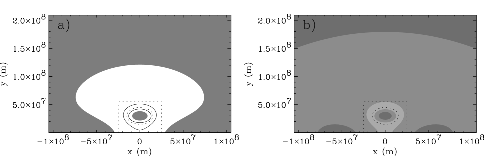
Fig. 6.: The plasma-$\beta$ (a) and Alfvén speed (b) in and near the prominence. In the left graph, gray denotes $\beta>1$. The solid line is the contour line $\beta=0.1$. In the right graph, darkest gray denotes $v_{\rm A}<c_{\rm s}$ and lightest gray denotes $v_{\rm A}>500$ km/s. Maximum Alfvén speed is $873$ km/s. The dotted circle represents the boundary of the prominence, the dotted rectangles the coronal surface over which the Poynting flux was integrated. The graphs are valid for $\rho_{\rm cor}=10^{-12}$ kg/m³. For other coronal densities the scalings $\beta\propto\rho_{\rm cor}$ and $v_{\rm A}\propto 1/\sqrt{\rho_{\rm cor}}$ can be used.

In addition, the effect of the photospheric boundary condition was studied. A perfectly reflecting photosphere does not allow a net momentum or energy flux. Also, the magnetic flux distribution is constant. The implementation of the photospheric boundary conditions automatically ensures zero momentum flux and constant magnetic flux. However, since the magnetic field is not symmetric in $y=0$, a small Poynting flux is present. Consider a box-shaped surface around the prominence. The coronal ‘walls’ of this surface each have a shortest distance to the prominence center of $2.5\times 10^{7}$ m (see Fig. 6) and reach down to the photosphere, along which we close the box. The total time-averaged Poynting flux through the photosphere is typically $10^{-3}-10^{-2}$ times smaller than the coronal flux, for vertical oscillations. For horizontal oscillations, the coronal flux is small in essence (due to the anti-symmetry) and provides no reasonable yardstick (of course one could still use the flux through a single ‘wall’, but this is bound to lead to similar results as for vertical oscillations). Furthermore, we point out that the equilibrium height of the prominence during oscillation studies does not change by more than 0.06%, and often even less. We therefore feel that the photospheric boundary is sufficiently well represented in our numerical boundary conditions.

4 Oscillation studies

Before we study oscillations in prominences, we first have to compute a stable, numerical prominence equilibrium.

Fig. 7.: The volume averaged horizontal and vertical momenta $\rho v_{x,y}$ as a function of time for all eight simulations. Curves with a higher initial value of the momentum correspond to larger coronal densities. All simulations were started with the same velocity perturbation (10 km/s). For the sake of clarity only the first $5000$ s are shown for the vertical momentum.

Table 1.: Characteristic time scales of prominence dynamics for all eight cases considered. The coronal density $\rho_{\rm cor}$ and (as a consequence) the prominence longitudinal mass density $\sigma$ are the only parameters that differ. In particular the total current $I_{0}=6.5\times\,10^{10}$ A and the initial perturbation ($10$ km/s) are the same for all simulations. The estimated error in the period is typically less than $3\%$, vertical periods having larger errors than horizontal periods. The estimated error in the damping time is typically less than $10\%$, vertical damping times having smaller errors than horizontal damping times. For the horizontal oscillations, we used only cases 1–6, for vertical oscillations only cases 1–5 to compare the numerical results to the simple line current model of Sect.2. No reliable vertical time scales could be obtained for the last two cases due to strong transients and noise.

	coronal density	prominence	effective	horizontal oscillations		vertical oscillations
Nr.	$\rho_{\rm cor}$ (kg/m3)	mass $\sigma$ (kg/m)	mass $\sigma_{\rm eff}$ (kg/m)	period (s)	damping (s)	period (s)	damping (s)
1	$1.25\times\,10^{-13}$	$1.28\times\,10^{4}$	$1.37\times\,10^{4}$	$2\,874$	$38\,500$	$1\,135$	$1\,564$
2	$2.5\times\,10^{-13}$	$1.29\times\,10^{4}$	$1.47\times\,10^{4}$	$2\,961$	$26\,600$	$1\,118$	$1\,100$
3	$5\times\,10^{-13}$	$1.31\times\,10^{4}$	$1.68\times\,10^{4}$	$3\,134$	$16\,100$	$1\,087$	$860$
4	$1\times\,10^{-12}$	$1.35\times\,10^{4}$	$2.13\times\,10^{4}$	$3\,461$	$9\,400$	$1\,053$	$820$
5	$2\times\,10^{-12}$	$1.42\times\,10^{4}$	$3.07\times\,10^{4}$	$4\,160$	$5\,600$	$1\,080$	$990$
6	$4\times\,10^{-12}$	$1.56\times\,10^{4}$	$5.04\times\,10^{4}$	$5\,600$	$3\,800$	$1\,350$	$1\,020$
7	$8\times\,10^{-12}$	$1.84\times\,10^{4}$	$9.20\times\,10^{4}$	$7\,740$	$8\,100$	??	??
8	$1.6\times\,10^{-11}$	$2.41\times\,10^{4}$	$17.95\times\,10^{4}$	$10\,300$	$22\,200$	??	??

For the coronal arcade, we choose the following parameter values: $H_{\rm d}=4\times\,10^{8}$ m, $M_{\rm d}=10^{20}$ Am and plasma-density $\rho_{\rm cor}=10^{-12}$ kg/m³. The two flux tubes are given by: $r_{0}=1.5\times\,10^{7}$ m, $\Delta r_{0}=10^{7}$ m and $j_{0}=2\times\,10^{-4}$ A/m². Hence the longitudinal mass density of the flux tube proper is $\sigma_{0}=1.28\times\,10^{4}$ kg/m, and the density of the prominence is $\sigma=1.35\times\,10^{4}$ kg/m. The total current is $I_{0}=6.5\times\,10^{10}$ A. Such a prominence is expected to oscillate with a horizontal period of 2777 s and a vertical period of 1118 s. The sound speed was chosen $c_{\rm s}=128.5$ km/s, typical of the corona at a temperature $T=10^{6}$ K.

We now let the initial state as defined in the previous section relax to a numerical equilibrium. The artificial damping term ($\partial_{t}\rho\mathchoice{\mbox{\boldmath$\displaystyle v$}}{\mbox{\boldmath$\textstyle v$}}{\mbox{\boldmath$\scriptstyle v$}}{\mbox{\boldmath$\scriptscriptstyle v$}}=-\alpha\rho\mathchoice{\mbox{\boldmath$\displaystyle v$}}{\mbox{\boldmath$\textstyle v$}}{\mbox{\boldmath$\scriptstyle v$}}{\mbox{\boldmath$\scriptscriptstyle v$}}$) was used to prevent numerical instabilities. We choose $\alpha=0.1$ for the first $10^{4}$ seconds of the relaxation, and $\alpha=0.01$ during the latter $10^{4}$ seconds. Figure 3 shows the relaxation of the volume averaged horizontal and vertical momentum. At the end of the relaxation the flows in the larger part of the arcade are typically less than 5 m/s. Along the boundary of the prominence body a rather irregular flow field exists with velocities of 175 m/s at most. The prominence still moves downwards at a systematic speed of some 1 m/s (see Fig. 4). Considering both the magnitude of the velocity perturbation applied later and the total simulation time scale, we consider these residual flows to be unimportant. The agreement between simulations starting from different relaxations (with a duration of either $9\,000$ or $20\,000$ s) confirm this.

Fig. 8.: Flow field of the plasma in the prominence and ambient corona, during the first 1600 s. Shown are the numerical results for $\rho_{\rm cor}=10^{-12}$ kg/m³, see Table 1. Maximal velocity is 11.7 km/s.

The numerical equilibrium does not deviate much from the initial state. The resulting field topology around the prominence is shown in Fig. 5. The prominence itself is a region of high plasma-$\beta$, surrounded by a region of magnetically dominated plasma (see Fig. 6). At large distances from the prominence the plasma-$\beta$ becomes larger than unity again, as the magnetic field strength decreases while the coronal density is constant (due to the absence of gravity). The Alfvén speed is also shown in Fig. 6. It increases as one approaches the prominence from the corona, once inside it falls off rapidly. The sound speed, of course, is the same everywhere (it is a free parameter of Eq. (10)).

The obtained numerical equilibrium is used to derive a series of numerical equilibria by adding (or subtracting) a constant value from the density in each cell. Since this does not create any additional forces (the force due to gas pressure is $-c_{\rm s}^{2}\nabla\rho$) a new equilibrium is found. In the resulting equilibria we disturb the inner part of the prominence (all plasma within $1.25\times\,10^{7}$ m from the center of mass) with a velocity perturbation of 10 km/s, at an angle of $45^{o}$ to the photosphere. The evolution of the system is studied for $10^{4}$ s, in some cases even for $2\times\,10^{4}$ s.

In Fig. 7 the evolution of the volume averaged momentum is shown for all eight cases considered. Initially momentum is concentrated in the prominence, but it is redistributed throughout the corona in the subsequent evolution. A global oscillation is apparent, whose properties depend strongly on coronal density.

For one particular case, the flow field is shown in Figs. 8 and 9. Although only the velocity is shown, the prominence stands out clearly in most graphs. It seems to move through the coronal plasma as a rigid body. The largest velocities are usually found outside the prominence. The coronal plasma ‘washes around the filament’.

Fig. 9.: Flow field of the plasma in the prominence and ambient corona, during the latter part of the evolution. Shown are the numerical results for $\rho_{\rm cor}=10^{-12}$ kg/m³, see Table 1. Maximal velocity is 8.5 km/s.

In particular, we studied the motion of the prominence. This was done by computing every so many time steps the center of longitudinal mass and current density. To rule out the contribution of the coronal part of the grid, only densities above a certain threshold where used. As the contrast between typical coronal and prominence current densities is larger than the contrast between typical coronal and prominence mass densities, the first provide a better estimate of the location of the prominence. Nevertheless, the results are always similar.

In essence, the motion of the filament can be described by two decoupled damped harmonic oscillators. The horizontal resp. vertical displacement of the center of longitudinal mass or current density of the prominence may be fitted to $A{\rm e}^{-t/T_{\rm damp}}\sin 2\pi t/P$. The resulting periods and damping times for the horizontal and vertical oscillations are listed in Table 1. Sometimes strong transient effects at the start of the simulation and noise at later times (when the velocities are smaller) cause deviations from a simple damped harmonic oscillator. The horizontal oscillations yield, in general, better fits. Typically the low density simulations lead to better fits than the high density simulations. For horizontal motions we used the cases 1–6, for vertical motions we used the cases 1–5 (see Table1). No reliable vertical time scales could be obtained for the last two cases due to strong transients and noise.

Comparing the results with simulations where a purely vertical or horizontal perturbation was applied shows that the horizontal and vertical motions of the filament are actually decoupled. This is understandable as the filament is located on the symmetry line of the coronal field (see also van den Oord et al.  1998). At the same time this suggests that non-linear effects are not important. Further evidence for the linearity of the numerical results is found in the good fits of the prominence oscillation curves to a damped harmonic oscillator. However, simulations with smaller or larger perturbations (3 km/s or 20 km/s instead of 10 km/s) yield different damping times for the horizontal motions (see Fig. 10). For all three simulations the horizontal periods differ by only $0.1\%$, while the horizontal damping times differ by $30-60\%$! Apparently, the horizontal damping mechanism depends non-linearly on the flow speeds. We have no explanation for this result, but believe it to be genuine. Extensive tests with higher spatial and temporal resolution argue strongly against the possibility of a numerical effect. It is a strong indication that the damping mechanism for horizontal and vertical motion differ, at least in their dependencies on the flow field.

Fig. 10.: The center of the current density above the threshold value. Dashed line: 20 km/s perturbation; solid line: 10 km/s perturbation; dotted line: 3 km/s perturbation. The first curve was multiplied by $0.5$, the last curve was multiplied by $3.333$ to facilitate comparison. The top graph shows the horizontal displacement, the bottom graph the vertical displacement. The coronal density equals $\rho_{\rm cor}=2.5\times\,10^{-13}$ kg/m³.

Fig. 11.: Periods for the horizontal (squares) and vertical (diamonds) oscillations. The dotted lines are the quasi-stationary periods for a prominence loaded with mass $\sigma=\sigma_{0}+\pi r_{0}^{2}\rho_{\rm cor}$. The top dashed line is the model for horizontal oscillations assuming that the actual oscillating body is larger than just the prominence proper. The bottom dashed line is the model for vertical oscillations using the effective longitudinal mass density $\sigma_{\rm eff}$ as determined from the horizontal oscillations.

Fig. 12.: Quality factors ($Q=\pi T_{\rm damp}/P$) for the horizontal (squares) and vertical (diamonds) oscillations.

The horizontal periods show a strong dependence on the coronal density, while the vertical periods are almost constant (Fig. 11). The quality factors (Fig. 12) of the horizontal oscillation are typically larger than four, and hence damping contributes little to the oscillation frequency (see Eq. (6)). The dotted lines (in Fig. 11) represent the undamped quasi-stationary period for a prominence with a longitudinal mass density of $\sigma=\sigma_{0}+\pi r_{0}^{2}\rho_{\rm cor}$. Clearly this is a bad fit to the numerical results for horizontal oscillations. Let us assume that, due to the magnetic structure, the actual oscillating body has a radius $r_{\rm eff}>r_{0}$. The actual oscillating body now has an effective longitudinal mass density $\sigma_{\rm eff}=\sigma_{0}+\pi r_{\rm eff}^{2}\rho_{\rm cor}$. From Eq. (6) we obtain

$$\frac{1}{\rho_{\rm cor}}\left(\frac{2\mu_{0}M_{\rm d}^{2}}{\pi^{3}}\frac{y_{0}}{(y_{0}+H_{\rm d})^{5}}P_{x}^{2}-\sigma_{0}\right)=\pi r_{\rm eff}^{2}$$ (17)

the left-hand-side of which can be fitted to a function of the form $C\rho_{\rm cor}^{\gamma}$. We find that $r_{\rm eff}=5.0\times\,10^{7}(\rho_{\rm cor}/10^{-12})^{0.04}$ m, weakly dependent on the coronal density. The typical radius $r_{\rm eff}=5.0\times\,10^{7}$ m agrees well with the location of the magnetic surface across which the connectivity of the field lines changes from closed field lines in the corona to field lines anchored in the photosphere. An even better approximation to this surface is obtained by taking into account the effect of induced mass as described by Landau & Lifschitz (1989, p. 29; see also Lamb 1945). For an incompressible, potential hydrodynamical flow the effective mass is the sum of the mass of the actual oscillating body ($\sigma_{0}+\pi r_{0}^{2}\rho_{\rm cor}$) plus the mass of the fluid displaced by the body. In that case $\sigma_{\rm eff}=\sigma_{0}+2\pi r_{\rm eff}^{2}\rho_{\rm cor}$ (note the factor 2!) and we find $r_{\rm eff}=3.5\times\,10^{7}(\rho_{\rm cor}/10^{-12})^{0.04}$ m.

In Fig. 13, we have plotted the ratio of vertical damping time to horizontal damping time. From Eqs. (2), (7) and (9) this ratio is proportional to $c_{x}/c_{y}$. Here $c_{x}$ is the typical wave speed for perturbations travelling parallel to the photosphere and $c_{y}$ is the typical wave speed for perturbations travelling perpendicular to the photosphere. For simplicity, we assume that the cross sections for both directions have the same $\rho_{\rm cor}$ dependence, but given the azimuthal invariance of the prominence flux tube this is probably a fair approximation. Now $c_{x}$ and $c_{y}$ are equal to either the slow cusp speed $c_{\rm T}$, the Alfvén speed $c_{\rm A}$ or the fast speed $c_{\rm f}$. In a low plasma-$\beta$ environment, the cusp speed equals the sound speed $c_{\rm s}$, while the fast speed equals the Alfvén speed $c_{\rm A}$. Hence $c_{x}/c_{y}\propto\rho_{\rm cor}^{-0.5},1$ or $\rho_{\rm cor}^{0.5}$ depending on whether slow, Alfvén or fast wave emission prevails in a certain direction. From the data, we find $c_{x}/c_{y}\propto\rho_{\rm cor}^{-0.53}$ which strongly suggests that slow wave emission damps horizontal motions, while Alfvén or fast wave emission damps vertical motions. Since the prominence moves vertically to the field lines in the latter case, fast waves are more likely.

Fig. 13.: Ratio of the damping times of vertical and horizontal oscillations. The solid line ($\propto\rho_{\rm cor}^{-0.53}$) is a fit to the data points (plus signs). The dotted lines are fits to $c_{x}/c_{y}\propto\rho_{\rm cor}^{-0.5},1$ or $\rho_{\rm cor}^{0.5}$ using the data point for $\rho_{\rm cor}=5\times\,10^{-13}$ kg/m³ as a gauge.

The conclusions regarding damping mechanisms can be substantiated further by comparing the relevant time scales for horizontal and vertical oscillations independently to the Eqs. (7) and (9) (see Fig. 14).

Fig. 14.: The effective longitudinal mass density $\sigma_{\rm eff}$ over the damping time $T_{\rm d}$ and coronal density $\rho_{\rm cor}$ for horizontal (squares) and vertical (diamonds) oscillations. The dotted lines are model fits to Eq.(18).

For the mass, we use the effective longitudinal mass density $\sigma_{\rm eff}$ as obtained previously. From Eq. (2) and either Eq. (7) or (9) we find

$$\frac{\sigma_{\rm eff}}{\rho_{\rm cor}T_{\rm damp}}=Ac,$$ (18)

the left-hand-side of which can be fitted to $C\rho_{\rm cor}^{\gamma}$. Here $A$ is the cross-section perpendicular to the direction of motion. For horizontal oscillations we find $c_{x}\propto\rho_{\rm cor}^{0.06\pm 0.06}$, and $A\approx 2\times\,10^{7}$ m². This suggests excitation of slow waves by horizontal motion of the prominence. For vertical oscillations $c_{y}\propto\rho_{\rm cor}^{-0.54\pm 0.04}$ which suggests excitation of fast waves by vertical motion of the prominence. Since the Alfvén speed varies in space, it is not possible to derive a value of $A$ from the product of $Ac$.

The cross-section $A$ for the horizontal damping mechanism yields a dimension for the oscillating body smaller than the extended size $r_{\rm eff}$ as obtained from the horizontal periods. This may be due to field line curvature. Since the size of the oscillating ‘solid’ body is determined by the field topology, Lorentz forces cause the waves that carry away momentum. However, Lorentz forces only act perpendicular to, not parallel to the field lines. Thus only perturbations of magnetic field with a strong vertical component can excite horizontally travelling waves.

5 Summary and conclusions

We have made a numerical investigation of prominence oscillations, by solving the isothermal MHD equations in two dimensions. First we computed a prominence equilibrium that is very similar to the Kuperus-Raadu (inverse polarity) topology. However, in our numerical equilibrium the prominence is not infinitely thin, but instead well resolved. From this equilibrium, we derived other equilibria with different coronal plasma densities. We then perturbed the system by instantaneously adding momentum to the prominence mass and followed the ensuing oscillations. The dependence of the characteristic time scales (periods and damping times) on the coronal plasma density was analyzed in terms of a solid body moving through a fluid. To our knowledge this is the first attempt at numerically simulating prominence oscillations.

In our numerical model, we ignored the effects of gravity and thermodynamics, for the sake of clarity and practicality. Also, up to now the numerical boundary conditions we are using do not seem to allow a stable gravitationally stratified corona.

We believe, however, that gravity and thermodynamics do not contribute significantly to the physics of the system. Gravity is of small consequence for the equilibrium of a Kuperus-Raadu prominence as detailed by van Tend & Kuperus (1978). Force balance is due to two Lorentz forces: one due to the coronal magnetic arcade, the other due to the photospheric flux conservation. The gravitational force can be ignored when describing global equilibrium. Furthermore, the scale height of a corona of $T=10^{6}$ K is $3\times\,10^{8}$ m, which is larger than the typical vertical size of prominences. The inclusion of gravity would change the appearance of the prominence into a slab, with prominennce matter accumulating in the pre-existing (!) dips in the magnetic field lines. The magnetic field configuration would hardly change.

Likewise, the absence of a thermally structured corona and prominence seems of only minor influence. The most important effect would be that a cool prominence will be heavier than a prominence of coronal temperatures. In our model this is balanced by the absence of a longitudinal field. As a consequence, the pinching effect of the azimuthal prominence field has to be balanced by gas pressure only (in real prominences the longitudinal field pressure contributes significantly). The total longitudinal mass density of our prominence ($\sim 1.3\times 10^{4}$ kg/m³) agrees well with that of a slab of height $5\times\,10^{7}$ m, width $6\times\,10^{6}$ m and density $5\times\,10^{-11}$ kg/m³. Oliver & Ballester (1996) studied the influence of the prominence-corona transition region (characterized by strong temperature gradients) and found that it mainly influences the prominence internal oscillations, but not the global oscillations.

We point out that the inclusion of both gravity and thermodynamics would give the prominence proper the appearance of a cool slab, suspended in the dips of the field lines belonging to the prominence current. Presumably this will not change the global oscillation discussed in this paper, since that mode is determined by the overall field structure.

The results indicate that, for typical coronal densities ($\rho_{\rm cor}=10^{-13}-10^{-12}$ kg/m³), the prominence structure can indeed be viewed as a solid body moving through a fluid. However, the mass of this solid body is determined by the magnetic topology, not the prominence proper. In particular, the mass of the body seems to be determined by coronal field lines that enclose the prominence proper. In a low plasma-$\beta$ environment this is to be expected. As a consequence, the total mass of the oscillating solid body is larger than the mass of the prominence proper.

Due to the symmetry of the system, horizontal and vertical prominence oscillations decouple. These oscillations can each be interpreted as the motion of a damped harmonic oscillator. The horizontal periods and the horizontal and vertical damping times can be explained by assuming that the actual oscillating structure is larger than the prominence proper, due to the magnetic field topology. Only the vertical periods do not agree with this model. They are nearly constant for different values of the coronal density and are best modelled by the oscillation of the prominence proper in a corona with vanishing plasma density ($\rho_{\rm cor}\downarrow 0$). For realistic coronal densities, the horizontal periods change with $3-15\%$ at most when taking the actual oscillating structure into account. However, for lower prominence longitudinal mass densities $\sigma$ in a stronger coronal background field (and hence larger prominence currents $I_{0}$), the effect will be much more pronounced.

Vertical oscillations lead to the emission of fast waves that carry momentum away from the prominence and damp the oscillation. Horizontal oscillations, on the other hand, lead to the emission of slow waves. These will damp the horizontal oscillation, but less effectively than fast waves ($Q_{x}>Q_{y}$).

The difference in wave emission between horizontal and vertical oscillations can be understood in terms of the coronal arcade in which the prominence is embedded. Due to the large scale height, the arcade field is close to horizontal near the prominence. Waves that travel in the vertical direction (up or down) therefor travel more or less perpendicular to the field lines and must be fast waves. Waves that travel in the horizontal direction travel along the field lines. They could be either Alfvén waves or magneto-acoustic waves. As regards excitation of the waves, it is obvious that the vertical motion of a prominence across field lines that are nearly horizontal will compress both gas and magnetic field and thus set off fast waves. The excitation of the magneto-acoustic slow waves (for our analysis strongly suggests they are slow waves) is not as well understood. But apparently the prominence acts as a piston during horizontal motions along magnetic field lines of the arcade.

We surmise that for smaller scale height of the arcade the slow waves might be replaced by fast waves.

• N.A.J. Schutgens was financially supported by the Netherlands Organisation for Scientific Research (NWO) under grant nr. 781-71-047. He gratefully acknowledges stimulating discussions with Max Kuperus and Bert van den Oord. The Versatile Advection Code (VAC) was developed by G. Tóth as part of the project on ‘Parallel Computational Magneto-Fluid Dynamics’, funded by the Netherlands Organisation for Scientific Research (NWO) Priority Program on Massively Parallel Computing, while he was working at the Astronomical Institute of Utrecht University. G. Tóth currently receives a post-doctoral fellowship (D25519) from the Hungarian Science Foundation (OTKA).

References

- 1 Balthasar H., Wiehr E., 1994, A&A 286, 639
- 2 Balthasar H., Knölker M., Stellmacher G., Wiehr E., 1986, A&A 163, 343
- 3 Balthasar H., Stellmacher G., Wiehr E., 1988, A&A 204, 286
- 4 Balthasar H., Wiehr E., Schleicher H., Wöhl H. 1993, A&A 277, 635
- 5 Bashkirtsev V.S., Mashnich G.P, 1993, A&A 279, 610
- 6 Brackbill J.U., Barnes D.C., 1980, J.Comput.Phys. 35, 426
- 7 Forbes T.G., 1990, J.Geophys.Res. 95,
- 8 Hyder C.L., 1966, Z. Astrophys. 63, 78
- 9 Joarder P.S., Roberts B., 1992a, A&A 256, 264
- 10 Joarder P.S., Roberts B., 1992b, A&A 261, 625
- 11 Joarder P.S., Roberts B., 1993, A&A 277, 225
- 12 Joarder P.S., Nakariakov V.M., Roberts B., 1997, Sol.Phys. 173, 81
- 13 Kaastra J., 1985, Solar Flares, an Electrodynamical Model, thesis Utrecht University, the Netherlands
- 14 Kleczek J., Kuperus M., 1969, Sol. Phys. 6, 72
- 15 Kuperus M., Raadu M.A., 1974, A&A 31, 189
- 16 Lamb H., 1945, Hydrodynamics, Dover Publications
- 17 Landau L.D., Lifschitz E.M., 1989, Fluid Mechanics, Pergamon Press
- 18 Mashnich G.P., Bashkirtsev V.S., 1990, A&A 235, 428
- 19 Mashnich G.P., Druzhinin S.A., Levkovsky V.I., 1993, A&A 269, 503
- 20 Molowny-Horas R., Oliver R., Ballester J.L., Baudin F., 1997, Sol.Phys. 172, 181
- 21 Oliver R., Ballester J.L., 1995, ApJ 448, 444
- 22 Oliver R., Ballester J.L., 1996, ApJ 456, 393
- 23 Oliver R., Ballester J.L., Hood A. W., Priest E. R., 1992, ApJ 400, 369
- 24 Oliver R., Ballester J.L., Hood A. W., Priest E. R., 1993, ApJ, 409, 809
- 25 Park Y.D, Yun H.S., Ichimoto K., 1995, JApA 16, 384
- 26 Ramsey H.E., Smith S.F., 1966, AJ 71, 197
- 27 Roberts B., Edwin P.M., Benz A.O., 1984, ApJ 279, 857
- 28 Schutgens N.A.J., 1997a, A&A 323, 969
- 29 Schutgens N.A.J., 1997b, A&A 325, 352
- 30 Suematsu Y., Yoshinaga R., Terao N., Tsubaki T., 1990, PASJ 42, 187
- 31 Sütterlin P., Wiehr E., Bianda M., Küveler G., 1997, A&A 321, 921
- 32 Thompson W.T., Schmieder B., 1991, A&A 243, 501
- 33 Tóth G., 1996, Astrophys. Lett. & Comm. 34, 245
- 34 Tóth G., 1997, Proceedings of High Performance Computing and Networking Europe 1997 Lecture Notes in Computer Science 1225, 253, Springer-Verlag
- 35 Tóth G., Odstrčil D., 1996, J. Comput. Phys. 128, 82
- 36 Tsubaki T., 1988, Altrock R.C. (ed), Proc. Sacramento Peak summer Workshop, p. 140
- 37 van den Oord G.H.J., Kuperus M., 1992, Sol. Phys. 142, 113
- 38 van den Oord G.H.J., Schutgens N.A.J., Kuperus M., 1998, A&A 339, 225
- 39 van Tend W., Kuperus M., 1978, Sol. Phys. 59, 115 59, 115
- 40 Zhang Y., Engvold O., 1991, Sol. Phys. 134, 275
- 41 Zhang Y., Engvold O., Keil S.L., 1991, Sol. Phys. 132, 63