Transport properties of degenerate electrons in neutron star envelopes and white dwarf cores

Abstract

New calculations of the thermal and electrical electron conductivities are performed for a broad range of physical parameters typical for envelopes of neutron stars and cores of white dwarfs. We consider stellar matter composed of astrophysically important chemical elements from H to Fe in the density range from $10^{2}$–$10^{4}\mbox{\leavevmode\nobreak\ g\,cm${}^{-3}$}$ up to $10^{7}$–$10^{10}\mbox{\leavevmode\nobreak\ g\,cm${}^{-3}$}$, where atoms are fully ionized and electrons are strongly degenerate. We have used modified ion structure factors suggested recently by Baiko et al. (1998). In the ion liquid, these modifications take into account, in an approximate way, instantaneous electron-band structures that reduce the electron-ion scattering rate. In crystallized matter, the new structure factors include multi-phonon processes important at temperatures not very much lower than the melting temperature $T_{\rm m}$. The transport coefficients obtained differ significantly from those derived earlier in the important temperature range $T_{\rm m}/5\la T\la 5T_{\rm m}$. The results of our numerical calculations are fitted by analytical expressions convenient for astrophysical applications.

1 Introduction

Thermal and electrical conduction in the envelopes of neutron stars and the cores of white dwarfs plays crucial role in many aspects of evolution of these stars. Thermal conductivity is the basic quantity needed for calculating the relationship between the internal temperature of a neutron star and its effective surface temperature; this relationship affects thermal evolution of the neutron star and its radiation spectra (e.g., Gudmundsson et al. gpe83 (1983); Page page97 (1997); Potekhin et al. pcy97 (1997), hereafter Paper I). Electrical conductivity is the basic quantity used in calculations of magnetic-field evolution in neutron star crusts (e.g., Muslimov & Page mp96 (1996); Urpin & Konenkov uk97 (1997); Konar & Bhattacharya kb97 (1997)). Thermal conductivity of degenerate matter is also an essential ingredient for white-dwarf pulsation modelling (e.g., Fontaine & Brassard fb94 (1994)).

For applications one should know the transport properties of dense stellar matter where electrons are strongly degenerate and form nearly ideal Fermi-gas, whereas ions are partially or fully ionized and form either a strongly coupled Coulomb liquid or a Coulomb crystal. Under such conditions, electrons are usually most important charge and heat carriers, and the electrical and thermal conductivities are mainly determined by electron scattering off ions (hereafter, ei scattering).

The conductivities of degenerate electrons due to ei scattering were studied in a number of papers. The general formalism, based on a variational method (Ziman Ziman (1960)), has been developed by Flowers & Itoh (fi76 (1976)) (see references to earlier results therein). Their numerical results, however, have been critically revised by Yakovlev & Urpin (yu80 (1980)), who developed a simple analytical description of the conduction due to ei scattering in dense Coulomb plasmas. The results by Yakovlev & Urpin (yu80 (1980)) were confirmed in detailed calculations for both solid (Raikh & Yakovlev ry82 (1982)) and liquid (Itoh et al. itoh-ea83 (1983); Nandkumar & Pethick np84 (1984)) regimes. Later Yakovlev (yak87 (1987)) calculated the electron transport coefficients in the liquid phase taking into account non-Born corrections. In Paper I, the authors performed extensive calculations of the same coefficients including additionally the effects of responsive electron background on the ion structure factors.

Itoh et al. (itoh-ea84 (1984, 1993)) improved the results by Yakovlev & Urpin (yu80 (1980)) and Raikh & Yakovlev (ry82 (1982)) in the solid regime by including the nuclear form factor $F(q)$ (where $\hbar q$ is a momentum transfer), in order to take into account finite sizes of atomic nuclei, and studied the role of the Debye–Waller factor $\mathrm{e}^{-2W(q)}$ (e.g., Kittel Kittel (1963)), which describes reduction of ei scattering rate in a crystal due to lattice vibrations. The Debye–Waller factor proved to be important at temperatures close to the melting temperature of a Coulomb crystal, and at sufficiently high densities, where zero-point vibrations are large. Later Baiko & Yakovlev (bya95 (1995, 1996)) made detailed Monte Carlo and analytical calculations of the electron transport in crystalline dense matter including the nuclear form factor and the Debye–Waller factor; they fitted the results by simple analytical expressions. These results were in reasonable agreement with those obtained by Itoh et al. (itoh-ea84 (1984, 1993)).

Nevertheless the transport theory developed in the cited articles possessed one important drawback: it predicted unrealistically large jumps (by a factor of 2–4) of the transport coefficients at the melting point in spite of the fact that many other physical properties of ion liquid and solid were very similar. This indicated that the theory was incomplete and had to be improved.

The improvements have been suggested recently by Baiko et al. (bkpy (1998)) (hereafter Paper II). In the solid regime, multi-phonon processes have been included in the electron-phonon scattering, whereas all previous calculations used the one-phonon approximation. Furthermore, it has been noted in Paper II, that the static structure factor of ions conventionally used in the liquid regime may require modification when applied to calculation of the electron scattering processes because of appearance of incipient ordered structures. The authors suggested an approximate treatment of this effect by subtracting a certain part from the static structure factor. Both modifications affect significantly the electron transport properties near the melting point and reduce the jumps of the transport coefficients.

In this paper, we apply the results by Baiko et al. (bkpy (1998)) to calculation of the electron electrical and thermal conductivities in a wide range of physical parameters typical for the envelope of a neutron star or the core of a white dwarf. We also derive an effective ei scattering potential that yields the conductivities in a simple analytical form, reproducing the numerical results within, at most, a few tens of percent in the whole of the physically meaningful range of the plasma parameters. Finally, we discuss the main features of the electron transport properties, and the role of various electron scattering mechanisms.

The paper is organized as follows. In Sect. 2 we introduce basic definitions and give a brief overview of the main features of electron conduction in different regimes. In Sect. 3 we describe our calculation of the electron transport coefficients and propose a fit to these coefficients. Numerical results are discussed in Sect. 4.

2 Dense degenerate matter

2.1 Equilibrium properties

Consider fully ionized degenerate stellar matter in the density range from about $10^{2}$–$10^{4}\mbox{\leavevmode\nobreak\ g\,cm${}^{-3}$}$ to $\sim 10^{10}\mbox{\leavevmode\nobreak\ g\,cm${}^{-3}$}$. For simplicity, we assume that there is one ion species at any given $\rho$ and $T$.

The state of degenerate electrons can be described by the Fermi momentum $p_{\rm F}$ or wave number $k_{\rm F}$:

$$p_{\rm F}=\hbar k_{\rm F}=\hbar\,(3\pi^{2}n_{\rm e})^{1/3}=m_{\rm e}cx_{\rm r},$$ (1)

where $n_{\rm e}$ is the electron number density, $m_{\rm e}$ is the electron mass, $x_{\rm r}\approx 1.009\,(\rho_{6}Z/A)^{1/3}$ is the relativistic parameter, $Z$ is the ion charge number, $A$ is the atomic weight, and $\rho_{6}$ is mass density $\rho$ in units of $10^{6}\mbox{\leavevmode\nobreak\ g\,cm${}^{-3}$}$. The electron degeneracy temperature is

$$T_{\rm F}=(\epsilon_{\rm F}-m_{\rm e}c^{2})/k_{\rm B}\approx 5.93\times 10^{9}\left(\sqrt{1+x_{\rm r}^{2}}-1\right)\mbox{\leavevmode\nobreak\ K},$$ (2)

where $k_{\rm B}$ is the Boltzmann constant and $\epsilon_{\rm F}=m_{\rm e}c^{2}\,\sqrt{1+x_{\rm r}^{2}}\equiv m_{\rm e}^{*}c^{2}$ is the electron Fermi energy. Our analysis is thus limited by the condition $T\ll T_{\rm F}$. It is also restricted to temperatures $T\la 5\times 10^{9}$ K at which atomic nuclei do not dissociate. Electrostatic screening properties of the electron gas are characterized by the Thomas–Fermi wave number $k_{\rm TF}$:

$$k^{2}_{\rm TF}=4\pi e^{2}\,{\partial n_{\rm e}\over\partial\mu}\approx{\alpha_{\rm f}\over\pi}\,{\sqrt{1+x_{\rm r}^{2}}\over x_{\rm r}}\,(2k_{\rm F})^{2},$$ (3)

where $\mu\approx\epsilon_{\rm F}$ is the electron chemical potential and $\alpha_{\rm f}=e^{2}/\hbar c=1/137.036$ is the fine-structure constant.

The state of ions (atomic nuclei) can be conveniently specified by the Coulomb plasma parameter

$$\Gamma={(Ze)^{2}\over k_{\rm B}Ta_{\rm i}}\approx{22.75\,Z^{2}\over T_{6}}\left({\rho_{6}\over A}\right)^{1/3},$$ (4)

where $e$ is the elementary charge, $a_{\rm i}=[3/(4\pi n_{\rm i})]^{1/3}$ is the ion-sphere radius, $n_{\rm i}=n_{\rm e}/Z$ is the number density of ions, and $T_{6}$ is temperature in units of $10^{6}$ K. If $\Gamma\ll 1$, ions are weakly coupled and form the Boltzmann gas. For $\Gamma\ga 1$, they constitute a strongly coupled liquid. Freezing occurs at a temperature $T_{\rm m}$ which corresponds to $\Gamma=\Gamma_{\rm m}$. For classical ions, $\Gamma_{\rm m}=172$, whereas quantum effects (zero-point ion vibrations) suppress the freezing and increase $\Gamma_{\rm m}$ (Nagara et al. nnn87 (1987)). The quantum effects become important at $T\ll T_{\rm p}$, where

$$T_{\rm p}=\hbar\omega_{\rm p}/k_{\rm B}\approx 7.832\times 10^{6}\,(Z/A)\rho_{6}^{1/2}\leavevmode\nobreak\ {\rm K}$$ (5)

is the ion plasma temperature, $\omega_{\rm p}=(4\pi Z^{2}e^{2}n_{\rm i}/m_{\rm i})^{1/2}$ is the ion plasma frequency, $m_{\rm i}=Am_{\rm u}$ is the ion mass, and $m_{\rm u}=1.6605\times 10^{-24}$ g is the atomic mass unit. Under realistic conditions, the quantum effects strongly suppress crystallization of hydrogen and helium plasmas, but do not affect significantly the melting of carbon and heavier elements (e.g., Chabrier chabr93 (1993)). However, they affect the properties of matter of any composition at $T\ll T_{\rm p}$.

2.2 Transport coefficients and structure factors

Electrical ($\sigma$) and thermal ($\kappa$) conductivities of degenerate electrons can be conveniently expressed through effective electron collision frequencies, $\nu_{\sigma}$ and $\nu_{\kappa}$, as (e.g., Ziman Ziman (1960); Yakovlev & Urpin yu80 (1980))

$$\sigma={n_{\rm e}e^{2}\over m_{\rm e}^{*}\nu_{\sigma}},\qquad\kappa={\pi^{2}k_{\rm B}^{2}Tn_{\rm e}\over 3m_{\rm e}^{*}\nu_{\kappa}}.$$ (6)

The collision frequencies are reduced to sums of partial collision frequencies associated with relevant electron scattering mechanisms which can be studied separately. This approximation is accurate to $\sim 1\%$ in the case of strongly degenerate electrons (e.g., Ziman Ziman (1960); Lampe lampe68 (1968)).

In the solid phase at $T\ll T_{\rm p}$, where the frequency of ei collisions $\nu_{\sigma,\kappa}^{ei}$ is strongly reduced, the electron transport is limited by scattering off various irregularities of the crystalline structure. The particular case of ion impurities, occasionally embedded in the lattice, was studied in detail by Itoh & Kohyama (ik93 (1993)) and will be taken into account in this article; in this case charge and heat transport are determined by a single collisional frequency $\nu_{\rm imp}$. On the other hand, in the liquid phase, at not very strong electron degeneracy for $Z\la 6$ the thermal (but not the electrical) conductivity may be affected by electron-electron (ee) collisions. The ee collision frequency $\nu^{ee}$ was evaluated, e.g., by Urpin & Yakovlev (uy80 (1980)), Timmes (timm92 (1992)), and in Paper I [see Eq. (32) below]. These results for electron-electron and electron-impurity scattering are not modified by the present consideration. The total effective collision frequencies are $\nu_{\sigma}=\nu_{\sigma}^{ei}$, $\nu_{\kappa}=\nu_{\kappa}^{ei}+\nu_{\kappa}^{ee}$ in the liquid and $\nu_{\sigma,\kappa}=\nu_{\sigma,\kappa}^{ei}+\nu_{\rm imp}$ in the solid.

We will focus on ei scattering. In a weakly coupled ion gas, $\Gamma\ll 1$, collective effects lead to a dynamical ion screening of ei interaction which can be described by the dynamical dielectric function formalism (e.g., Williams & DeWitt wdw69 (1969)). In a strongly coupled ion liquid, it is customary to use the static structure factor of ions in order to describe the correlation effects (Hubbard hubb66 (1966)). This description, however, does not apply to quantum liquids, such as H or He at high densities (e.g., Chabrier chabr93 (1993)). In crystalline matter, ei interaction is adequately described in terms of absorption and emission of phonons (Abrikosov abrik61 (1961)). The description can be realized using a dynamical structure factor of ions (Flowers & Itoh fi76 (1976)).

The ei collision frequencies can be expressed through dimensionless Coulomb logarithms $\Lambda_{\sigma,\kappa}$ (cf. Yakovlev & Urpin yu80 (1980)):

$$\nu^{ei}_{\sigma,\kappa}={4\pi Z^{2}e^{4}n_{\rm i}\over p_{\rm F}^{2}v_{\rm F}}\,\Lambda_{\sigma,\kappa}={4Z\epsilon_{\rm F}\over 3\pi\hbar}\,\alpha_{\rm f}^{2}\Lambda_{\sigma,\kappa},$$ (7)

where $v_{\rm F}=p_{\rm F}/m_{\rm e}^{\ast}$ is the electron Fermi velocity.

For a strongly coupled plasma of ions ($\Gamma\ga 1$), the Coulomb logarithms calculated in the variational approach (with the simplest trial functions, Ziman Ziman (1960)) in the Born approximation read

$$\Lambda_{\sigma,\kappa}=\int_{q_{0}}^{2k_{\rm F}}{\rm d}q\,q^{3}u^{2}(q)\,S_{\sigma,\kappa}(q)\,\left[1-{v_{\rm F}^{2}\over c^{2}}\left({q\over 2k_{\rm F}}\right)^{2}\right],$$ (8)

where $q_{0}$ is the cutoff parameter, equal to zero for the liquid phase and to the equivalent radius of the Brillouin zone $q_{\rm B}=(6\pi^{2}n_{i})^{1/3}$ in the solid phase. The latter cutoff filters out umklapp electron-phonon processes, which operate at $q>q_{\rm B}$ and give the main contribution to $\Lambda_{\sigma,\kappa}$, from normal processes, that take place at $q<q_{\rm B}$ and are negligible under the conditions of study (e.g., Baiko & Yakovlev bya95 (1995)). Furthermore, $u(q)\equiv|U(q)|/(4\pi Ze^{2})$, $U(q)$ is the Fourier transform of the elementary ei scattering potential, the factor in square brackets describes kinematic suppression of backward scattering of relativistic electrons (e.g., Berestetskii et al. LaLi-QED (1982)), and $S_{\sigma,\kappa}(q)$ are the effective static structure factors which take into account ion correlations, as discussed below.

In order to take into account corrections to the Born approximation, we multiply additionally the integrand in Eq. (8) by the ratio of the exact cross section of Coulomb electron scattering to the Born cross section. This approximate treatment of non-Born corrections was proposed by Yakovlev (yak87 (1987)) and used in Paper I. The corrections are significant for $Z\ga 20$ and $\rho\ga 10^{6}\mbox{\leavevmode\nobreak\ g\,cm${}^{-3}$}$.

In the case of Coulomb scattering, one has

$$u(q)={F(q)\over q^{2}|\varepsilon(q)|},$$ (9)

where $\varepsilon(q)$ is a static longitudinal dielectric function of the electron gas (Jancovici janco62 (1962)), describing electron screening of the scattering potential. The static ($\omega\to 0$) approximation of electron screening is adequate as long as typical energies transferred $\hbar\omega$ are small compared with $\hbar qv_{\rm F}$, which is the case, since the momentum transfer $\hbar q\sim p_{\rm F}$. At densities $\rho<10^{10}$ g cm^-3 and under the condition of full ionization, one can safely set the ion form factor $F(q)$ equal to 1, which corresponds to point-like nuclei.

The structure factors in Eq. (8) are given by (Paper II)

$$S_{\sigma}(q)\,\, =\,\, \int_{-\infty}^{+\infty}{\rm d}\omega\,S^{\prime\prime}(q,\omega)\,{z\over 1-\mathrm{e}^{-z}},$$ (10)

$$S_{\kappa}(q)\,\, =\,\, S_{\sigma}(q)+\left({3k_{\rm F}^{2}\over q^{2}}-\frac{1}{2}\right)\delta S_{\kappa}(q),$$ (11)

$$\delta S_{\kappa}(q) = \int_{-\infty}^{+\infty}{\rm d}\omega\,S^{\prime\prime}(q,\omega)\,{z^{3}\over 1-\mathrm{e}^{-z}}.$$ (12)

In this case $z=\hbar\omega/(k_{\rm B}T)$ and $S^{\prime\prime}(q,\omega)$ is the inelastic part of the total dynamical structure factor $S(q,\omega)=S^{\prime\prime}(q,\omega)+S^{\prime}(q)\delta(\omega)$, whereas the elastic part, $S^{\prime}(q)\delta(\omega)$, describes Bragg diffraction. When interaction of electrons with a crystalline lattice is considered, the Bragg diffraction leads to appearance of electron band structure (Bloch states) but does not contribute to electron transport (e.g., Flowers & Itoh fi76 (1976)). If $z$ values “allowed” by $S^{\prime\prime}(q,\omega)$ in Eqs. (10)–(12) are small, as it happens for scattering in a classical Coulomb system [i.e., at $T\ga T_{\rm p}$; cf. Eq. (18)], we can pull the other functions containing $z$ out of the integral setting $z=0$. Then $\delta S_{\kappa}(q)$ vanishes, and $S_{\sigma}(q)=S_{\kappa}(q)=S^{\prime\prime}(q)$, where $S^{\prime\prime}(q)=\int_{-\infty}^{+\infty}S^{\prime\prime}(q,\omega){\rm\,d}\omega$ is the inelastic part of the static structure factor. In this case the variational solution that is used in Eq. (8) becomes exact.

In the liquid phase, $\Gamma<\Gamma_{\rm m}$, it is only the static structure factor in the classical regime $S(q)=\int^{+\infty}_{-\infty}{\rm d}\omega S(q,\omega)$ (e.g., Young et al. ycdw91 (1991) and references therein) that has been determined quite accurately. Thus we will consider only classical liquids, $T\ga T_{\rm p}$. In the solid phase $S(q,\omega)$ was calculated with reasonable accuracy in Paper II, which enables us to study the transport properties of quantum and classical solids.

3 Calculation of electron conductivities

3.1 Solid phase

The dynamical structure factor of a Coulomb crystal has been calculated in Paper II in the harmonic-lattice approximation, taking into account explicitly multi-phonon processes. For $q>q_{\rm B}$ the inelastic part may be written as

$$S^{\prime\prime}(q,\omega)\,\, \!\!\!= \!\!\!{\mathrm{e}^{-2W(q)-\hbar\omega/(2k_{\rm B}T)}\over 2\pi}\int^{+\infty}_{-\infty}\!\!\!\!\!\!{\rm d}t\,\mathrm{e}^{-{\rm i}\omega t}K(q,T,t),$$ (13)

$$K(q,T,t) = \exp\left[{\hbar q^{2}\over 2m_{\rm i}}\left\langle{\cos{\omega_{\nu}t}\over\omega_{\nu}\sinh{(z_{\nu}/2)}}\right\rangle_{\rm ph}\right]-1,$$ (14)

where $\langle\ldots\rangle_{\rm ph}$ denotes averaging over the phonon spectrum in the first Brillouin zone, and

$$W(q)={3\hbar\over 2m_{\rm i}}\left\langle{(\@vec{q}\cdot\@vec{e}_{\nu})^{2}\over\omega_{\nu}}\left(\bar{n}_{\nu}+\frac{1}{2}\right)\right\rangle_{\rm ph}.$$ (15)

In this case, $\nu\equiv(\@vec{Q},s)$, $s=1,2,3$ enumerates phonon polarizations, $\@vec{Q}$ is a phonon wave vector, $\@vec{e}_{\nu}$ the polarization vector, $\omega_{\nu}$ the frequency, and $\bar{n}_{\nu}=\left(\mathrm{e}^{z_{\nu}}-1\right)^{-1}$ is the mean number of phonons, $z_{\nu}=\hbar\omega_{\nu}/(k_{\rm B}T)$. For the lattice types of interest [e.g., body centred cubic (bcc) or face centred cubic (fcc) ones], $W(q)=r_{T}^{2}q^{2}/6$, where $r_{T}^{2}$ is the mean-squared ion displacement. Thus $W(q)$ does not depend on the orientation of $\@vec{q}$. An analytical fit to $W(q)$ was proposed by Baiko & Yakovlev (bya95 (1995)):

$$W(q)=\frac{1}{4}\alpha_{1}\left(u_{-1}\,\mathrm{e}^{-9.1\eta}+2\eta\,u_{-2}\right),$$ (16)

where $\eta=T/T_{\rm p}$, $u_{n}=\langle(\omega_{\nu}/\omega_{p})^{n}\rangle_{\rm ph}$ is a frequency moment of Coulomb lattice ($u_{-2}=13.0$ and $u_{-1}=2.8$ for bcc lattice, cf. Pollock & Hansen ph73 (1973)), and

$$\alpha_{1}=\alpha_{0}\,{q^{2}\over 4k_{\rm F}^{2}},\qquad\alpha_{0}={4k^{2}_{\rm F}a^{2}_{i}\over 3\Gamma\eta}=1.683\sqrt{{x_{\rm r}\over AZ}}.$$ (17)

It is possible to derive an asymptote of $S^{\prime\prime}(q,\omega)$, Eq. (13), for $T\gg T_{\rm p}$ (classical solid) and for $|\omega|\gg\omega_{\rm p}$. Expanding $\cos{\omega_{\nu}t}\approx 1-(\omega_{\nu}t)^{2}/2$ and $\sinh{(z_{\nu}/2)}\approx z_{\nu}/2$ and noting that the second term in Eq. (14) does not contribute into $S^{\prime\prime}(q,\omega)$ at these frequencies, we obtain

$$S^{\prime\prime}(q,\omega)\approx{1\over\sqrt{\pi}\,qv_{T}}\exp\left(-{\omega^{2}\over q^{2}v^{2}_{T}}-{\hbar\omega\over 2k_{\rm B}T}\right),$$ (18)

where $v_{T}=\sqrt{2k_{\rm B}T/m_{\rm i}}$ is the thermal ion velocity. Thus in a classical solid the collisional energy transfer is limited either by $\hbar qv_{T}$ or by $\hbar\omega_{\rm p}$, in both cases being smaller than $k_{\rm B}T$. Therefore only the values $z\ll 1$ contribute to the integrals (10), (12) in this case.

In the general case of classical or quantum Coulomb crystals, the effective structure factors (10) and (12) can be written as (Paper II)

$$S_{\sigma}(q)\,\, \!= {1\over 2}\,\mathrm{e}^{-2W(q)}\int_{-\infty}^{+\infty}{{\rm d}x\over\cosh^{2}x}\,K(q,T,t),$$ (19)

$$\delta S_{\kappa}(q) = \mathrm{e}^{-2W(q)}\int_{-\infty}^{+\infty}{\rm d}x\,{1-2\sinh^{2}x\over\cosh^{4}x}\,K(q,T,t),$$ (20)

where $x=\pi tT/\hbar$. We have calculated $S_{\sigma}(q)$ and $\delta S_{\kappa}(q)$ for the bcc lattice and fitted them by the expressions

$$S_{\sigma}(q)\,\, \!= \mathrm{e}^{-2W(q)}\left(\mathrm{e}^{2W_{1}(q)}-1\right),$$ (21)

$$\delta S_{\kappa}(q) = \alpha_{1}\left[{91\,\eta^{2}\,\mathrm{e}^{-2W(q)}\over(1+111.4\eta^{2})^{2}}\right.$$ (22)

$$+ \left.{0.101\,\eta^{4}\over(0.06408+\eta^{2})(0.001377+\eta^{2})^{3/2}}\right],$$

$$W_{1}(q) = {\alpha_{1}\,u_{-2}\,\eta^{2}\over 2\,\sqrt{\eta^{2}+(u_{-2}/117)^{2}}}.$$

These fits cover a wide range of the parameters, $0.001\leq\eta\leq 10$ and $0\leq\alpha_{1}\leq 0.3$, sufficient for calculation of transport coefficients. Equations (21) and (22) reproduce also the asymptotes of the effective structure factors at low and high $\eta$ which can be obtained from Eqs. (19) and (20). The maximum fit error, equal to 4%, occurs for $\alpha_{1}=0.001$, and $\eta=0.04$.

We have also calculated the effective structure factors for fcc Coulomb lattice and the results appear to be almost indistinguishable from those obtained for bcc lattice. Therefore, the electron transport coefficients are insensitive to the lattice type, and we will calculate them for bcc lattice.

3.2 Liquid phase

In the classical liquid, we employ the static structure factor, $S(q)$, obtained by Rogers and DeWitt (unpublished) for the one-component classical plasma of ions in a rigid electron background by solving the modified hypernetted-chain (MHNC) equations (Rosenfeld & Ashcroft ra79 (1979)), and fitted by Young et al. (ycdw91 (1991)) in the range $1\leq\Gamma\leq 225$. For calculating ei scattering rates, we have modified these structure factors by subtracting the contribution of elastic scattering as prescribed in Paper II:

$$S_{\sigma,\kappa}(q)=S(q)-\mathrm{e}^{-2W(q)}(2\pi)^{3}n_{i}\sum_{\@vec{G}\neq 0}\overline{\delta(\@vec{q}-\@vec{G})},$$ (23)

where the sum is over all non-zero reciprocal lattice vectors $\@vec{G}$, and the upper bar means averaging over orientations of $\@vec{q}$. This modification is meant to account for instantaneous electron band-structures which emerge in a strongly coupled Coulomb liquid because of local temporary crystal-like ordering. In this context, the choice of the lattice type and corresponding vectors $\@vec{G}$ is ambiguous, but the Coulomb logarithms are insensitive to it.

Since our consideration is based on the classical static structure factor $S(q)$, we obtain $\Lambda_{\sigma}=\Lambda_{\kappa}$ and $\nu^{ei}_{\sigma}=\nu^{ei}_{\kappa}$ in the liquid regime. This is justified because we typically have $T\ga T_{\rm p}$, for the cases under study (see below). Nevertheless we could easily incorporate the quantum effects into the calculation, were the quantum dynamical structure factors $S(q,\omega)$ available for ion fluid.

Note that in Paper I the Coulomb logarithms in the ion liquid were calculated with $S(q)$ obtained for a polarizable electron background including the local field corrections. The effect of the response of the background appeared to be noticeable for H and He plasmas only. We neglect this effect in the present calculations because our consideration of ion liquid for light elements is approximate anyway due to the neglect of quantum corrections to $S(q)$.

For light elements, the highest temperatures corresponding to the liquid regime, $\Gamma\geq 1$, are much below $T_{\rm F}$. Accordingly, there exists a temperature range where $T<T_{\rm F}$ and $\Gamma<1$. In this interval the formalism of the effective structure factors does not provide an accurate treatment of ion screening. For $\Gamma\leq 0.25$, the Coulomb logarithms were calculated in Paper I taking into account dynamical character of ion screening at $\Gamma\ll 1$ and $k_{\rm TF}\ll k_{\rm F}$ (e.g., Williams & DeWitt wdw69 (1969)):

$$\Lambda_{\sigma,\kappa} = \ln\left({2k_{\rm F}\over q_{\rm D}}\right)-{\zeta\over 2}\,\ln\left({1\over\zeta}\right)+{1+\zeta\over 2}\,\ln\left({1\over 1+\zeta}\right)$$ (24)

$$-v_{\rm F}^{2}/(2c^{2})+\beta/2,$$

$q_{\rm D}=\sqrt{3\Gamma}/a_{i}$ is the inverse Debye screening length of ion gas, $\zeta=(k_{\rm TF}/q_{\rm D})^{2}$, and $\beta=\pi\alpha_{\rm f}Zv_{\rm F}/c$; $\beta/2$ is a lowest-order non-Born correction in the weak electron-screening approximation (Yakovlev yak87 (1987)).

The Coulomb logarithms in the transition domain from weak ($\Gamma\ll 1$) to strong ($\Gamma\ga 1$) ion coupling can be calculated using the formalism by Boerker et al. (brdw82 (1982)). We do not apply this formalism, but the Coulomb logarithms calculated at $\Gamma\leq 0.25$ and at $\Gamma\geq 1$ converge nicely and can be fitted in a unified manner. This convergence deteriorates at lower $\rho\sim 10$–100  g cm^-3, because electron screening ceases to be weak ($k_{\rm TF}\sim k_{\rm F}$), and Eq. (24) becomes inaccurate.

3.3 Numerical results and fitting formulae

Using the effective structure factors $S_{\sigma,\kappa}(q)$ described above, we have calculated the Coulomb logarithms $\Lambda_{\sigma,\kappa}$ for $Z$ from 1 to 26 and for mass numbers $A$ corresponding to the most abundant isotopes. The mass density $\rho$ varied from $10\mbox{\leavevmode\nobreak\ g\,cm${}^{-3}$}$ for $Z=1,2$ and from $100\mbox{\leavevmode\nobreak\ g\,cm${}^{-3}$}$ for $Z\geq 3$ to $10^{10}\mbox{\leavevmode\nobreak\ g\,cm${}^{-3}$}$; the coupling parameter $\Gamma$ varied from 1 to $10^{4}$ for $Z<20$ and to $10^{5}$ for $20\leq Z\leq 26$. The physically meaningful domain of the parameters is constrained by several conditions. First, it is assumed that the atoms are fully ionized (for a treatment of the case of partial ionization, see below). Secondly, light elements are not present at very high densities and temperatures since they burn into heavier ones. Thirdly, our calculation in the liquid phase is confined to the classical regime ($T\ga T_{\rm p}$), where the quantum corrections to the ion structure factors are neglected. Fourthly, electrons are assumed to be degenerate ($T\ll T_{\rm F}$). Finally, the present formalism appears to be invalid at very low temperatures, $T\ll T_{\rm p}Z^{1/3}e^{2}/(\hbar v_{\rm F})$, where the electron band-structure effects strongly reduce ei scattering rate (e.g., Raikh & Yakovlev ry82 (1982)), which is not taken into account in Eq. (8).

For practical applications, especially for modelling thermal and magnetic evolution of the neutron stars, as well as pulsations of the white dwarfs, it is desirable to have analytical formulae for the transport coefficients, rather than tables, graphs or cumbersome theoretical expressions. Analytical formulae for $\sigma$ and $\kappa$ were presented in several papers based on the earlier theoretical results described in Sect. 1 (Flowers & Itoh fi81 (1981); Yakovlev & Urpin yu80 (1980); Itoh et al. itoh-ea93 (1993); Baiko & Yakovlev bya95 (1995); Paper I). As our present results are significantly different, we propose new analytical expressions, which combine reasonable accuracy with simplicity.

Instead of constructing ad hoc fits to the numerical values of $\sigma$ and $\kappa$, we have chosen to devise an effective ei-scattering potential that would allow us to perform explicit analytical integration in Eq. (8) and that would reproduce correctly the familiar limiting cases: the case of Debye ion screening in a weakly-coupled plasma and the case of scattering by high-temperature phonons. In the first case, $u^{2}(q)S(q)$ in Eq. (8) should be replaced by $(q^{2}+q_{\rm s}^{2})^{-2}$, where $q_{\rm s}$ is the inverse screening length. In the second case (at $T_{\rm p}\la T\leq T_{\rm m}$), ei scattering rate is determined by $u^{2}(q)S^{\prime\prime}(q)$, where $u^{2}(q)\approx(q^{2}+k_{\rm TF}^{2})^{-2}$, and $S^{\prime\prime}(q)$ is the approximate effective static structure factor (Paper II) which can be written as $S^{\prime\prime}(q)\approx 1-\exp[-u_{-2}a_{\rm i}^{2}q^{2}/(3\Gamma)]$. This approach ensures that the analytical limits mentioned above are reproduced automatically by the fit expression.

We propose the following form of the effective potential in Eq. (8):

$$\left[u^{2}(q)S_{\sigma,\kappa}(q)\right]_{\rm eff}={1-\mathrm{e}^{-w(q)}\over(q^{2}+q_{\rm s}^{2})^{2}}\,G_{\sigma,\kappa}(\eta,\beta)D(\eta),$$ (25)

where $\mathrm{e}^{-w(q)}$ plays role of an effective Debye–Waller factor at large $\Gamma$ and is negligible at $\Gamma<1$, $q_{\rm s}$ is an effective screening wave number, $D(\eta)$ is associated with the quantum correction to the Debye–Waller factor, and $G_{\sigma,\kappa}(\eta,\beta)$ is a phenomenological factor that describes reduction of thermal ion displacements in quantum solid at $T\la T_{\rm p}$ and contains non-Born corrections expressed through the argument $\beta$ [see Eq. (24)]. Our numerical results are reproduced with the following choice of $q_{\rm s}$, $w(q)$ and $G_{\sigma,\kappa}(\eta,\beta)$:

$$q_{\rm s}^{2} = (q_{\rm i}^{2}+k_{\rm TF}^{2})\,\mathrm{e}^{-\beta},$$ (26)

$$q_{\rm i}^{2}(\Gamma) = q_{\rm D}^{2}\,(1+0.06\,\Gamma)\,\mathrm{e}^{-\sqrt{\Gamma}},$$ (27)

$$w(q) = u_{-2}(q/q_{\rm D})^{2}\,(1+\beta/3),$$ (28)

$$G_{\sigma}(\eta,\beta) = {\eta\over\sqrt{\eta^{2}+\eta_{0}^{2}}}\,(1+0.122\beta^{2}),\quad\eta_{0}={0.19\over Z^{1/6}},$$ (29)

$$G_{\kappa}(\eta,\beta) = G_{\sigma}(\eta,\beta)+0.0105\left(1-Z^{-1}\right)$$ (30)

$$\times\left[1+\left({v_{\rm F}\over c}\right)^{3}\beta\right]{\eta\over(\eta^{2}+0.0081)^{3/2}},$$

$$D(\eta) = \exp\left(-\alpha_{0}u_{-1}\,\mathrm{e}^{-9.1\eta}/4\right),$$ (31)

where $\alpha_{0}$ is given by Eq. (17). Inserting Eq. (25) into Eq. (8), we arrive at the analytical expressions for the Coulomb logarithms presented in the Appendix.

The typical error of our fits in the physically reasonable range of parameters is 3% (maximum 6%) for $Z\geq 20$ and gradually increases with decreasing $Z$. The maximum error occurs for low $Z$ at the melting point in the high-density region, where our formulae interpolate across the conductivity jump discussed in the next section. For instance, a typical error for carbon plasma is 8% and the maximum is 22% at the highest density ($\rho=10^{9}\mbox{\leavevmode\nobreak\ g\,cm${}^{-3}$}$) and $\Gamma=\Gamma_{\rm m}$.

Finally, let us outline the case of multicomponent ion mixtures. Actually the case deserves a separate study and we treat it approximately here. At least for $T\ga T_{\rm p}$, it would be a good approximation to replace $Z^{2}n_{i}\Lambda_{ei}\to\sum_{j}Z_{j}^{2}n_{j}\Lambda_{ej}$ in Eq. (7), where summation is over all ion species $j$, and the Coulomb logarithm $\Lambda_{ej}$ depends generally on $j$. In a strongly coupled ion system we recommend to calculate $\Lambda_{ej}$ from Eqs. (1), (26)–(31) with $Z=Z_{j}$ and $\Gamma_{j}=Z_{j}^{5/3}e^{2}(4\pi n_{\rm e}/3)^{1/3}(k_{\rm B}T)^{-1}$ (the ion-coupling parameter for ion species $j$). The latter expression is prompted by the “additivity rule” that is highly accurate for thermodynamic functions of multicomponent ion mixtures (Hansen et al. hansen-ea77 (1977)).

Another option is to adopt the widely used mean-ion approximation. In the latter approximation, the plasma is treated as a mixture of electrons and one ionic species, with an effective charge $eZ_{\rm eff}$ equal to an average charge of all ions at different ionization stages. The mean-ion approximation can be used also in the regime of partial ionization (cf. Paper I).

Figure 1: Dependence of the electrical conductivity produced by ei scattering on temperature (lower horizontal scale) or Coulomb coupling parameter (upper horizontal scale) in carbon plasma at $\rho=10^{4}$ g cm^-3. Filled circles show the present numerical results, and the solid line is given by our fitting formula. The dashed line is obtained under traditional assumptions (see the text) and exhibits a jump at the melting point. Dotted lines are obtained including electron scattering by ¹⁶O impurities with concentrations $x_{\rm imp}=0.02$ and 0.04.

4 Discussion of the results

Figure 2: Same as in Fig. 1 but for the thermal conductivity.

Fig. 1 shows the temperature dependence of the electrical conductivity of degenerate electrons in a carbon plasma at $\rho=10^{4}$ g cm^-3. Fig. 2 shows the same dependence of the thermal conductivity. Upper horizontal scale indicates corresponding values of the ion coupling parameter $\Gamma$. Since the ion charge number is rather low, $Z=6$, non-Born corrections are insignificant. All the data presented in the figures, except dotted lines, show the conductivities produced solely by ei scattering.

Filled circles display our present numerical values of the conductivities, while solid lines are the analytical fits. Dashed lines show the ‘old’ conductivities calculated using the approximations which have been widely employed in the previous works (Sect. 1): the one-phonon approximation in the solid phase and use of the total (inelastic + elastic) ion structure factor in the liquid phase. One can see large jumps of the ‘old’ curves at the melting point. These jumps were present for all elements and for all plasma parameters, and they were typically a factor of 2–4 in magnitude (Itoh et al. itoh-ea93 (1993)). The modification of the structure factors improves the treatment of the conductivities both in the liquid and solid phases of strongly-coupled ion system (Sects. 3.1 and 3.2) and makes the jumps almost invisible for different chemical elements in a broad range of densities. This has allowed us to produce the unified fits which are equally valid in solid and liquid matter.

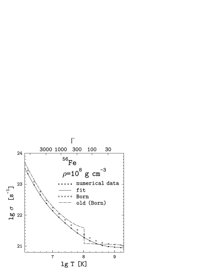
Figure 3: Electrical conductivity produced by ei scattering in Fe matter at $\rho=10^{8}$ g cm^-3 vs temperature or Coulomb coupling parameter. Filled circles show the present numerical results, and the solid line is the fit (non-Born corrections included). Open circles are the present results but in the Born approximation. The dashed line is the old result in the Born approximation.

Nevertheless, our calculations do show large jumps of the conductivities at the melting point at high densities, where zero point vibrations become important. We suggest that these jumps are artificial and come from using classical ion structure factors in ion liquid (Sect. 3.2) under the conditions in which quantum effects in liquid are really important. On the other hand, the quantum effects are properly included in our calculations for crystalline matter. Since the numerical data used for constructing the fitting formulae include both phases, liquid and solid, the fitting of these data by the unified analytical expressions shifts the conductivities in the liquid phase closer to those in the solid phase. Therefore we expect that the fits in the high-density ion liquid give more reliable electron conductivities than our original numerical data. This assumption will be checked in the future when the structure factors in ion liquid are calculated taking into account the quantum effects.

Dotted lines in Figs. 1 and 2 show the effect of another electron scattering mechanism – scattering by charged impurities (Sect. 2.2). We have assumed an admixture of oxygen nuclei with concentrations 2% and 4%. Electron-impurity scattering is seen to have little effect on the conductivities at high temperatures, but it becomes dominant scattering mechanism at $T\ll T_{\rm p}$.

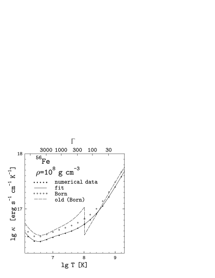
Figure 4: Same as in Fig. 3 but for the thermal conductivity.

Figs. 3 and 4 are analogous to Figs. 1 and 2 and show the temperature dependence of the conductivities produced by ei scattering in iron plasma at $\rho=10^{8}$ g cm^-3. Filled dots are our numerical results and solid lines are the fits. One can again see large jumps of the traditional conductivities at the melting point, and the smooth character of the improved curves. For elements with high $Z$ (like Fe), the non-Born corrections become important in a dense plasma (Yakovlev yak87 (1987)). To illustrate this effect, open circles display results of our calculations in the Born approximation. The non-Born corrections are seen to increase the ei collision frequency (decrease the conductivities) by about 20–30%. The corrections become lower when density decreases below $10^{6}$ g cm^-3. Dashed lines show the ‘old’ conductivities calculated in the Born approximation. The divergence between the ‘old’ and new results in the Born approximation, seen in Fig. 4 at relatively low temperatures, is caused by a not very accurate determination of the low-temperature ($T\ll T_{\rm p}$) asymptote of an effective electron-phonon potential in the ‘old’ results by Baiko & Yakovlev (bya95 (1995)).

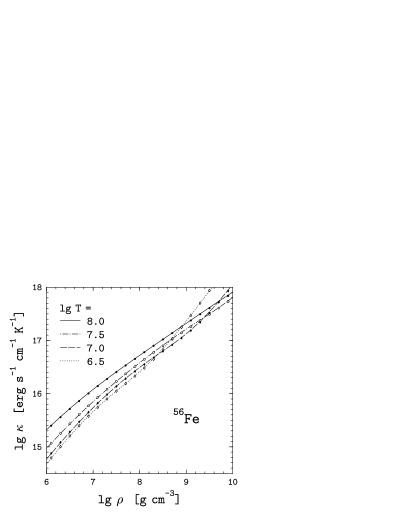
Figure 5: Thermal conductivity vs density in iron plasma at several $T$. Various symbols show numerical results, and curves are the fits. Conductivity due to ee collisions is included but is entirely unimportant. Impurities are neglected.

The density dependence of the thermal conductivity at several values of $T$ is displayed in Figs. 5 and 6. Fig. 5 shows the thermal conductivity of iron plasma in the density range appropriate to the outer envelope of a neutron star at $\lg T$[K]= 6.5, 7.0, 7.5 and 8.0. Fig. 6 shows the thermal conductivity of matter composed of H, He, C, Fe at $T=10^{7}$ K in about the same density range (related to the outer envelope of a neutron star or to the core of a white dwarf). We assume that no impurities are present, but we include the contribution of ee scattering in addition to the ei scattering. The ee scattering contributes to $\nu_{\kappa}$, i.e, lowers the thermal conductivity. According to Paper I,

$$\nu^{ee}={3\alpha_{\rm f}^{2}\,(k_{\rm B}T)^{2}\over 2\pi^{3}\,\hbar m_{\rm e}^{\ast}c^{2}}\left({2k_{\rm F}\over k_{\rm TF}}\right)^{3}J(x_{\rm r},y),$$ (32)

where $y=\sqrt{3}\,T_{\rm pe}/T$, $T_{\rm pe}=(\hbar/k_{\rm B})\,\sqrt{{4\pi e^{2}n_{\rm e}/m_{\rm e}^{\ast}}}$ is the electron plasma temperature, and

$$J(x_{\rm r},y) \approx \left(1+{6\over 5x_{\rm r}^{2}}+{2\over 5x_{\rm r}^{4}}\right)\,\left[{y^{3}\over 3(1+0.07414\,y)^{3}}\right.$$ (33)

$$\times\ln\left(1+{2.81\over y}-{0.81\over y}\,{v_{\rm F}^{2}\over c^{2}}\right)$$

$$\left.+{\pi^{5}\over 6}\,{y^{4}\over(13.91+y)^{4}}\right].$$

For a plasma of light elements, $Z\la 6$, the strongest effect of the ee collisions takes place at temperatures comparable to degeneracy temperature $T_{\rm F}$ (Lampe lampe68 (1968); Urpin & Yakovlev uy80 (1980)), as confirmed by Fig. 6. For Fe matter, ee collisions are unimportant. For H and He plasmas, their effect is more pronounced at lower $\rho$, where the chosen temperature, $T=10^{7}$ K, is closer to $T_{\rm F}$. We conclude that ee collisions do not play a leading role in thermal transport by degenerate electrons but should be taken into account in a plasma composed of light elements.

Figure 6: Thermal conductivity vs density in matter of different chemical composition (H, He, C, Fe) at $T=10^{7}$ K. Filled circles are numerical values and curves are fits. Lower curves and circles are calculated including ei and ee collisions, while upper curves and circles take account of ei collisions alone.

The strong effect of chemical composition (Fig. 6) is related to the $Z$-dependence of the collision frequencies $\nu^{ei}_{\sigma,\kappa}$. The higher is $Z$, the larger is $\nu^{ei}_{\sigma,\kappa}$, and the lower is the conductivity. Comparing Figs. 5 and 6 we see that a temperature variation by a factor of 30 can change the thermal conductivity of iron plasma much less than altering the chemical composition from H to Fe at fixed $T$. This effect has important consequences for the relationship between surface and internal temperatures of neutron stars (Paper I).

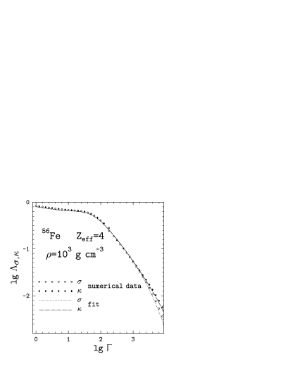
Figure 7: Coulomb logarithms versus effective Coulomb coupling parameter for a partially ionized iron plasma with effective charge $Z_{\rm eff}=4$ at $\rho=10^{3}$ g cm^-3 in the mean-ion approximation.

Finally let us consider partially ionized matter. We expect that this case can be considered in the mean-ion approximation (Sect. 3.3). Fig. 7 shows the dependence of the Coulomb logarithms $\Lambda_{\sigma}$ and $\Lambda_{\kappa}$ on the effective Coulomb plasma parameter $\Gamma=Z_{\rm eff}^{2}e^{2}(4\pi n_{\rm i}/3)^{1/3}(k_{\rm B}T)^{-1}$ for a partially ionized Fe matter at $\rho=10^{3}$ g cm^-3 and $Z_{\rm eff}=4$. The assumption that $Z_{\rm eff}$ is independent of temperature is unrealistic, and we adopt it for illustration only. Open and filled symbols show numerical values of $\Lambda_{\sigma}$ and $\Lambda_{\kappa}$, respectively, calculated in the mean-ion approximation, while dotted and dashed lines are the fit curves. Although we did not include the data with $Z\ll A/2$ in the fitting, our fit formulae appear to be robust and reproduce them quite well.

5 Conclusions

We have reconsidered the electrical and thermal conductivities of degenerate electrons produced by ei scattering, using the modified structure factors of ions as suggested in Paper II. We have analysed the electron transport in a wide range of densities, from about $10^{2}-10^{4}\mbox{\leavevmode\nobreak\ g\,cm${}^{-3}$}$ to $\sim 10^{7}-10^{10}\mbox{\leavevmode\nobreak\ g\,cm${}^{-3}$}$, and temperatures $T\sim 10^{4}-10^{9}$ K, for chemical compositions of astrophysical importance. The obtained conductivities differ significantly from those calculated previously in a wide range of temperatures, $T_{\rm m}/5\la T\la 5T_{\rm m}$, near the melting temperature $T_{\rm m}$ of Coulomb crystals. Our new approach has reduced unrealistically large jumps of the transport coefficients at the melting point obtained in the earlier works. This, in turn, allowed us to develop a unified description of electron conduction in liquid and crystal matter and obtain an effective potential for the ei interaction.

The ei scattering, which we studied in this article, is known to be the most important mechanism of electron relaxation under prevailing physical conditions in the envelopes of neutron stars and in the cores of white dwarfs. We expect that the improved transport coefficients can be used to solve various problems of the physics of neutron stars and white dwarfs (cooling, evolution of accreting stars, nuclear burning of matter, pulsation modes, evolution of magnetic fields, etc.).

Appendix: analytical fits to Coulomb logarithms

Carrying out the integration in Eq. (8) with the effective potential given by Eq. (25) yields the following expressions for the Coulomb logarithms, which enter Eq. (7) for the effective collision frequencies:

$$\Lambda_{\sigma,\kappa}^{\rm fit}=\left[\Lambda_{1}(s,w)-{v^{2}\over c^{2}}\Lambda_{2}(s,w)\right]G_{\sigma,\kappa}(\eta,\beta).$$ (1)

Here $s=q_{\rm s}^{2}/(2k_{\rm F})^{2}$, $w=w(2k_{\rm F})$ [see Eqs. (26)–(31)],

$$2\Lambda_{1}(s,w) = \ln{s+1\over s}+{s\over s+1}\,(1-\mathrm{e}^{-w})$$ (2)

$$- (1+sw)\,\mathrm{e}^{sw}\left[{\rm E}_{1}\,(sw)-{\rm E}_{1}\,(sw+w)\right],$$

$$2\Lambda_{2}(s,w) = \!\!{\mathrm{e}^{-w}-1+w\over w}-{s^{2}\over s+1}(1-\mathrm{e}^{-w})-2s\ln{s+1\over s}$$ (3)

$$+ s(2+sw)\,\mathrm{e}^{sw}\left[{\rm E}_{1}\,(sw)-{\rm E}_{1}\,(sw+w)\right],$$

and $E_{1}(x)=\int^{\infty}_{x}y^{-1}\mathrm{e}^{-y}{\rm\,d}y$ is the exponential integral given, for example, by the rational-polynomial approximations in Abramowitz & Stegun (Abramowitz (1972)).

In the particular case of $s\ll 1$ and $s\ll w^{-1}$, numerical cancellation of large numbers can be avoided with aid of the asymptotic expressions

$$\Lambda_{1}(s\to 0,w) = \frac{1}{2}\left[E_{1}(w)+\ln w+\gamma\right],$$ (4)

$$\Lambda_{2}(s\to 0,w) = {\mathrm{e}^{-w}-1+w\over 2w},$$ (5)

where $\gamma=0.5772\ldots$ is the Euler’s constant.

In the limiting case of $w\ll 1$, we obtain

$$\Lambda_{1}(s,w\ll 1) \approx w\left({2s+1\over 2s+2}-s\,\ln{s+1\over s}\right),$$ (6)

$$\Lambda_{2}(s,w\ll 1) \approx w\left({1-3s-6s^{2}\over 4s+4}+\frac{3}{2}\,\ln{s+1\over s}\right).$$ (7)

In the opposite case of $w\gg 1$, the familiar expressions for the Debye-like screening are recovered:

$$\Lambda_{1}(s,w\gg 1) = \frac{1}{2}\left(\ln{s+1\over s}-{1\over s+1}\right),$$ (8)

$$\Lambda_{2}(s,w\gg 1) = {2s+1\over 2s+2}-s\,\ln{s+1\over s}.$$ (9)

References

- (1) Abramowitz M., Stegun I.A. (eds.), 1972, Handbook of Mathematical Functions, Dover, New York
- (2) Abrikosov A.A., 1961, Sov. Phys.–JETP 12, 1254
- (3) Baiko D.A., Yakovlev D.G., 1995, Astron. Lett. 21, 702
- (4) Baiko D.A., Yakovlev D.G., 1996, Astron. Lett. 22, 708
- (5) Baiko D.A., Kaminker A.D., Potekhin, A.Y., Yakovlev, D.G. 1998, Phys. Rev. Lett. 81, 5556 (Paper II)
- (6) Berestetskii V.B., Lifshitz E.M., Pitaevskii L.P. 1982, Quantum Electrodynamics, Pergamon, Oxford
- (7) Boerker D.B., Rogers F.J., DeWitt H.E., 1982, Phys. Rev. A 25, 1623
- (8) Chabrier G., 1993, ApJ 414, 695
- (9) Flowers E., Itoh N., 1976, ApJ 206, 218
- (10) Flowers E., Itoh N., 1981, ApJ 250, 750
- (11) Fontaine G., Brassard P., 1994, White dwarf seismology: Influence of the constitutive physics on the period spectra. In: Chabrier G., Schatzman E. (eds.) The Equation of State in Astrophysics, Cambridge Univ. Press, Cambridge, p. 347
- (12) Gudmundsson E.H., Pethick C.J., Epstein R.I., 1983, ApJ 272, 286
- (13) Hansen J.P., Torrie G.M., Vieillefosse P., 1977, Phys. Rev. A 16, 2153
- (14) Hubbard W.B., 1966, ApJ 146, 858
- (15) Itoh N., Kohyama Y., 1993, ApJ 404, 268; erratum 420, 943
- (16) Itoh N., Mitake S., Iyetomi H., Ichimaru S., 1983, ApJ 273, 774
- (17) Itoh N., Kohyama Y., Matsumoto N., Seki M., 1984, ApJ 285, 758
- (18) Itoh N., Hayashi H., Kohyama Y., 1993, ApJ 418, 405
- (19) Jancovici B., 1962, Nuovo Cim. 25, 428
- (20) Kittel C., 1963, Quantum Theory of Solids, Wiley, New York
- (21) Konar S., Bhattacharya D., 1997, MNRAS 284, 311
- (22) Lampe M., 1968, Phys. Rev. 170, 306
- (23) Muslimov A., Page D., 1996, ApJ 458, 347
- (24) Nagara H., Nagata Y., Nakamura T., 1987, Phys. Rev. A 36, 1859
- (25) Nandkumar R., Pethick C.J., 1984, MNRAS 209, 511
- (26) Page D., 1997, ApJ 479, 43
- (27) Pollock L.E., Hansen J.P., 1973, Phys. Rev. A 8, 3110
- (28) Potekhin A.Y., Chabrier G., Yakovlev D.G., 1997, A&A 323, 415 (Paper I)
- (29) Raikh M.E., Yakovlev D.G., 1982, Ap&SS 87, 193
- (30) Rosenfeld Y., Ashcroft N.W., 1979, Phys. Rev. A 20, 1208
- (31) Timmes F.X., 1992, ApJ 390, L107
- (32) Urpin V., Konenkov D., 1997, MNRAS 292, 167
- (33) Urpin V.A., Yakovlev D.G., 1980, SvA 24, 126
- (34) Williams R.H., DeWitt H.E., 1969, Phys. Fluids 12, 2326
- (35) Yakovlev D.G., 1987, SvA 31, 347
- (36) Yakovlev D.G., Urpin V.A., 1980, SvA 24, 303
- (37) Young D.A., Corey E.M., DeWitt H.E., 1991, Phys. Rev. A44, 6508
- (38) Ziman J.M., 1960, Electrons and Phonons, Oxford Univ. Press, Oxford