Image subtraction with non-constant kernel solutions.

Abstract

It is demonstrated that non-constant kernel solution, that can fit the spatial variations of the kernel can be obtained with minimum computing time. The CPU cost required with this new extension of the image subtraction method is almost the same as for fitting constant kernel solution. The method is demonstrated with a serie of Monte-Carlo images. Differential PSF variations and differential rotation between the images are simulated. It is shown that this new method is able to achieve an optimal results even in these difficult cases. It is clear that the most frequents instrumental problems are automatically corrected by the method. It is also demonstrated that the method does not suffer problems with under-sampling of the images. To conclude the method is applied to real images of crowded field. It is proved that much larger sub-areas of the images can be used for the fit, while keeping the same accuracy in the subtracted image. This result is especially important in case of variables located in low density fields, like the Huchra lens. Many other useful applications of the method are possible for major astrophysical problems. For instance supernovas search should benefit the method, but other applications like Cepheids surveys in other galaxies should also find some advantage in using the method. Many other applications will certainly show-up, since variability search is a major issue in astronomy.

1 INTRODUCTION

The way variability is analyzed in astronomical images has been deeply influenced by the developpement of the microlensing experiments, EROS (Aubourg 1993), OGLE (Udalski et al. 1994), MACHO (alcock et al. 1993), DUO (Alard & Guibert 1997) . The enormous quantity of CCD images produced by these experiments motivated the developpement of fast and accurate techniques to analyze variability. The first implementations of variability search were based on an analysis of catalogues of stellar objects. The production of the catalogues has been almost exclusively done using the DoPHOT software (Schechter & Mateo 1993). This type of analysis is still used in microlensing experiments, and proved very successful. However since we are concerned only with differential photometry, such data processing fails to be optimal. Purely differential methods like image subtraction seems to be better suited for study of variability in astronomical images. However the developpement of image subtraction technique has been long delayed by the inherent difficulty and complexity of the method. The first successful implementation of the method has been performed by Tomaney & Crotts (1996). Further progress have been made by the creation of fast optimal image subtraction (OIS) method (Alard & Lupton 1998). Due to its ability to solve the full least-square problem, the OIS method proved to produce subtracted images and light curves with an accuracy approaching closely the photon noise limit. The OIS method is very efficient for crowded stellar fields, like those encountered in microlensing experiments, and could readily be used for massive processing of microlensing data. The current implementation of the OIS works by dividing the field into small sub-areas where constant kernel solution are derived. In dense crowded fields, sub-areas as small as 128 $\times$ 128 pixels can be used, at this scale kernel variations can be ignored to a good approximation. However in case of very bad optics or of less dense fields, the constant kernel approximation does not hold any more. For instance, in high latitude fields taken for supernovae search, one does not encountered a sufficient number of bright objects to take an area small enough to ignore the kernel variations. We are then naturally conducted to try to make a self consistent fit of the kernel variations, as described in Alard & Lupton (1998). Although, it is important to notice that even if the spatial variations are fitted to order 1 only, the cost to build the least-square matrix will be about 9 times larger than for the constant kernel solution. Some situations might require order 2 or 3 or even more. Order 3 requires roughly 100 times more calculation than the constant kernel solution. We see that the problem becomes quickly UN-tractable, and that one of the main advantages of the OIS, the fast computing time will be completely lost. Fortunately, it will be demonstrated in this article that the fit of the spatial variations of the kernel can be achieved for little additional computing cost, provided some reanalysis of the problem.

2 Basic equations.

Here we remind briefly the basics of image subtraction (Alard & Lupton 1998). The essence of the method is to find a convolution kernel ($K$), that will transform a reference image ($R$) to fit a given image $I$.
In terms of least-squares this is equivalent to look for a kernel that will minimize the sum:

$$\sum_{i}\left([R\otimes K](x_{i},y_{i})-I(x_{i},y_{i})\right)^{2}$$ (1)

Provided the kernel is decomposed on basis of function, the above equation become a simple linear least-square problem. For the kernel decomposition we take:

$$K(u,v)=\sum_{n}a_{n}\ K_{n}(u,v)$$

with:

$$K_{n}(u,v)=e^{-(u^{2}+v^{2})}\ u^{i}\ v^{j}$$

The kernel solution can be calculated by solving the following linear system:

$$M\bf a=\bf B$$ (2)

With:

$$M_{ij}=\int[R\otimes K_{i}](x,y)\ \frac{[R\otimes K_{j}](x,y)}{\sigma(x,y)^{2}}\ dxdy$$

And:

$$B_{i}=\int I(x,y)\ \frac{[R\otimes K_{i}](x,y)}{\sigma(x,y)^{2}}\ dxdy$$

Additional linear parameters can be included to fit the differential background variations between the images. For details see Alard & Lupton (1998).

3 Solving for non-constant kernel solution with minimum computing time.

Most of the computing time involved in the computation of the kernel solution is spend in the calculation of the least-square matrix. The solution of the linear system itself takes an almost negligible amount of time. The computing time to build the matrix goes like the square of the number of coefficients. Thus the problem is that if we introduce new coefficients in order to fit the kernel variations, the cost of the calculation will become quickly prohibitive. To be more specific, let’s derive analytical formula’s for the spatial variations of the kernel. At each position (x,y) we can develop the kernel on the basis of function $K_{n}$. Thus the coefficients $a_{n}$ will be function of (x,y). Consequently the kernel can be written:

$$K(u,v)=\sum_{n}a_{n}(x,y)\ K_{n}(u,v)$$

We assume that the coefficients $a_{n}$ are smooth function of x and y. For simplicity we adopt a polynomial function of degree $d_{1}$.

$$a_{n}(x,y)=\sum_{i,j}b_{i,j}\ x^{i}\ y^{j}$$

Let’s calculate the relevant Least-square vectors:

$$V_{n}(x,y)=\ W_{m}(x,y)\times P_{q}(x,y)$$

With:

$$W_{m}(x,y)=\frac{[R\otimes K_{m}](x,y)}{\sigma(x,y)}$$

$$P_{q}(x,y)=x^{i}\ y^{j}$$

And:

$$q=i+j\times d_{1}$$

$$nc_{1}=\frac{(d_{1}+1)(d_{1}+2)}{2}$$

$$n=q\ +\ m\times nc_{1}$$

The elements of the least-square matrix can be expressed as scalar products of the Least-square vectors:

$$M_{n1,n2}=\int W_{m1}(x,y)\ W_{m2}(x,y)\ P_{q1}(x,y)\ P_{q2}(x,y)\ dxdy$$

The previous integral extend over all the image. However, we can always imagine to split the integration domain into small rectangular sub-areas. Within such small areas, one can always assume that the kernel is constant. It corresponds to approximate locally x, and y by the coordinates of the centers of the sub-areas, ($x_{k}$, $y_{k}$).
Considering this approximation the matrix elements can be written:

$$M_{n1,n2}=\sum_{k}Q_{m1,m2}^{k}(x,y)\ P_{q1}(x_{k},y_{k})\ P_{q2}(x_{k},y_{k})$$ (3)

With the following definition for the integral in the rectangular domain $D_{k}$:

$$Q_{m1,m2}^{k}=\int_{D_{k}}W_{m1}(x,y)\ W_{m2}(x,y)\ dxdy$$

A similar method can be applied to expand the vector on the right hand side of eq. 2.

$$B_{n}=\sum_{k}\ W_{m}^{k}(x,y)P_{q1}(x_{k},y_{k})$$ (4)

With:

$$W_{m}^{k}(x,y)=\int_{D_{k}}I(x,y)\ \frac{W_{m1}(x,y)}{\sigma(x,y)}\ dxdy$$

We see that the matrix elements corresponding to fitting the spatial variations of the kernel can be deduced the matrix elements $Q_{m1,m2}^{k}$ for only the cost of a summation over the number of sub-areas. The matrix $Q_{m1,m2}^{k}$, corresponds to the constant kernel solution, and has a much smaller number of elements than the matrix $M_{n1,n2}^{k}$. Once $Q_{m1,m2}^{k}$ has been estimated, $M_{n1,n2}$ can be calculated using the expansion given in Eq. 3. This procedure results in a drastic economy in computing time, since the summation inside the individual sub-areas are avoided for the calculation of the matrix elements. Using Eq. 4 the same type of expansion applies also to the calculation of the vector $B_{n}$. Since the individual sub-areas should be slightly larger than the kernel, a typical number for the surface of a sub-area is $30\times 30$ pixels. It means that in computing application we save a factor of about 1000 in the calculation of the matrix elements of the matrix $M_{n1,n2}$ which corresponds to the spatial variations. In practice, fitting the kernel variations costs only about 20 % more than making a constant kernel fit.

In high latitude fields, the only useful areas are those centered on bright (high S/N) objects. It usually results in a drastic reduction in the number of pixels to fit. Even in crowded fields, most of the information is contained in some high density regions. Thus in practise the fit can be restricted to a fraction of the image.

Of course, differential fitting of the background variations between the images can be included, exactly in the same way as was done for constant kernel solutions.

4 numerical simulations.

4.1 Test with variable PSF.

4.1.1 The simulated images.

To check the ability of the method to reconstruct the spatial variations of the kernel, a serie of test are performed with simulated images. The images are generated by putting stars randomly in the image, with a magnitude distribution corresponding to a bulge luminosity function. Noise is added in the images according to Poisson statistics. For the reference image we take a constant gaussian PSF:

$$\Phi_{0}(u,v)=e^{-\alpha(u^{2}+v^{2})}$$

In our simulation we take $\alpha=0.5$.
For the other image we simulate a variable PSF by taking the sum of 2 gaussians with different width and a relative weighting which is function of the position in the image. We also introduce a normalization factor for conservation of the flux.

$$\Phi(u,v)=\frac{e^{-\alpha(u^{2}+v^{2})}+r(x,y)\times e^{-\frac{\alpha(u^{2}+v^{2})}{4}}}{1+4\ r(x,y)}$$

For the spatial variation we take:

$$r(x,y)=\frac{0.25\ y}{w}$$

Where $w$ is the size of the simulated image.
The resulting images are presented in Fig. 1.

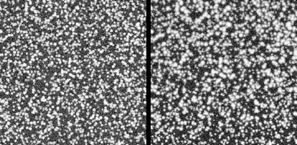
Figure 1: Simulation of crowded fields images. Left is the image with constant PSF, and next is the image with PSF variations along the Y axis. Note the large amplitude of the PSF variations. A total of 2500 stars has been included in this simulation.

4.1.2 Image subtraction.

First, a subtracted image with constant kernel solution has been produced. We use a set of parameter for the kernel that is similar to Alard & Lupton (1998), except that one basis function a delta function has been added to the kernel representation. Using a delta function might be useful in case the image have very similar seeing (Wozniak 1998). For the fit with with variable kernel solution we used a polynomial of order 2, since the variations of the coefficients of the PSF function are nearly parabolic. The resulting subtracted images are presented in Fig. 2.

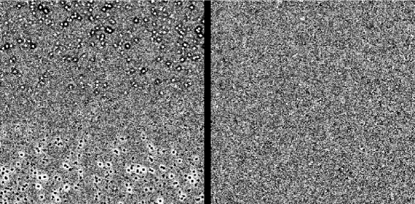
Figure 2: Left is the subtracted image obtained with constant kernel solution. Note the systematic pattern along the Y axis due to the kernel variations. Just next we present the subtracted image obtained by fitting the spatial variations of the kernel to order 2.

4.1.3 Noise estimation.

Noise in the subtracted image has 2 origins, the noise in the image to fit, and the noise in the reference image convolved with the kernel solution . In our images the Poisson noise can be extremely well approximated locally by a gaussian distribution with $\sigma=\sqrt{N}$. However this is not true for the reference image, since it has been transformed by convolution. The noise in the convolved image can be estimated in a straightforward way. The convolution will result in the combination of different Gaussian distribution, with differents $\sigma$ and weights. We keep the same notations, $I$ is the image to fit $R$ is the reference image, and we define the $IC$ which is the reference image convolved with the kernel solution.

$$IC_{i}=\sum_{j}R_{i-j}\ K_{j}$$

The combination of gaussian distribution will result in a gaussian distribution, and the resulting $\sigma$ of the distribution can be estimated by calculating the variance:

$$\sigma_{i}^{2}=\sum_{j}var(R_{i-j})\ K_{j}^{2}=\sum_{j}R_{i-j}\ K_{j}^{2}$$

Thus we see that the local variance of the image can be estimated by convolving the image with a filter that is just the square of the initial convolution filter. Consequently what we call Poisson deviation will be defined as:

$$\delta=\sqrt{\sigma_{i}^{2}+I_{i}}$$

The histograms of the pixels in the subtracted images normalized by the Poisson deviation are presented in Fig. 3. It is interesting to note that order 2 is sufficient to produce a Chi-square per degree of freedom (Chi2/Dof) which is extremely close to 1.

Figure 3: Histograms of the normalized deviations in the subtracted images presented in Fig. 2. Left is the histogram for constant kernel solution, and right is the histogram for a fit of kernel variation to order 2. The pixels in the subtracted images have been normalized by the Poisson deviations (see text for details). The dashed curve is gaussian with $\sigma=1$.

4.2 Checking the ability of the method to correct the astrometric registration.

Image registration is performed by calculating a polynomial transform from the positions of brights objects. However, there is no guarantee that this procedure is optimal. In case the image registration to the reference frame is not perfect, a simple translation can be taken into account by a constant kernel solution. However more complex features like differential rotation, or differential distortion between the images cannot be corrected with constant kernel solution. But they can be corrected with non-constant kernel solution. We will illustrate this fact by simulating differential rotation between 2 images. We keep the reference image we had already generated for the previous simulations, and make another one by rotating the frames with respect to its center with an amplitude of 0.7 pixel from one corner to the other corner of the frame. The result of subtraction are presented in Fig. 4. The systematic pattern due to rotation appears clearly in the image with constant kernel solution, while it is completely removed in the fit of a solution with a spatial variation of order 2. This is well confirmed by the Chi-square analysis which shows that an optimal result has been reached with the non-constant kernel solution (see Fig. 5).

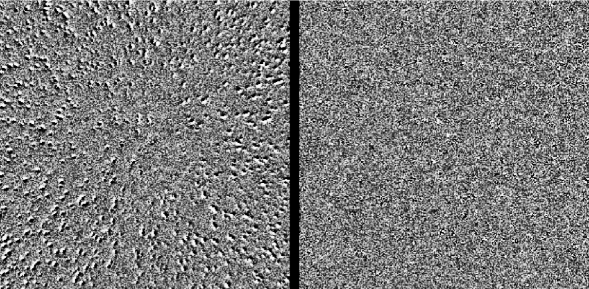
Figure 4: Image subtraction in case of images mis-aligned by differential rotation. Left is the subtracted image obtained with constant kernel solution. Note the systematic pattern due to the differential rotation between the images. Next is the subtracted image obtained by fitting the spatial variations of the kernel to order 2. Note the complete diseaperance of the systematic patterns.

Figure 5: Histograms of the normalized deviations in the subtracted images presented in Fig. 4. Left is the histogram for constant kernel solution, and right is the histogram for a fit of kernel variation to order 2. The dashed curve is gaussian with $\sigma=1$. Note the goodness and the dramatic reduction of the Chi-square when fitting the kernel variations.

4.3 Under-sampling.

One last problem that can be encountered in astronomical images is under-sampling. To test the sensitivity of the method to under-sampling, we simulate a pair of very under-sampled images. We take $\alpha=2.0$ ($FWHM=1.17$ pixels) for the reference and $\alpha=1.0$ ($FWHM=1.67$ pixels) for the other image. Since our goal is just to test the effect of under-sampling only, we perform image subtraction with constant kernel solution. The resulting normalized Chi-square distribution is presented in Fig. 6. The result is as good as in previous simulations. One may wonder why under-sampling does not induce any problem, since under-sampling should affect the convolution with the basis vectors. It is true that individually the least-square vectors which are obtained with under-sampled images will differ from the well sampled vectors. However one may not forget that the best solution is constructed by taking linear combinations of the least-square vectors. Even if the vectors are slightly different from the well sample vectors, an optimal linear combination of these vectors can be made anyway.

Figure 6: Histograms of the deviations in the subtracted image for simulated, very under-sampled images. The PSF in the reference image is very narrow with: $FWHM=1.17$ pixels, thus we are in presence of a bad case of under-sampling. For the other image $FWHM=1.67$, consequently it is also under-sampled.

5 Testing with astronomical images.

It was already shown in Alard & Lupton (1998) that nearly optimal results (Chi2/Dof = 1.05) could be achieved within a small sub-area of a crowded field. This is of course not true if the area is extended, since kernel variations are not negligeable any more. However, by using a variable kernel solution, one should be able to get a result closely similar for a larger region to what had been obtained for a small area. We test this assumption by extracting 2 larger sub-areas ($256\times 256$) from the fields already used in Alard & Lupton (1998), and making image subtraction with constant and variable kernel solutions. The results are shown in Fig. 7 and Fig. 8. The constant kernel solution achieved only Chi2/Dof = 1.19, with numerous systematic residuals near the edges of the field. On the contrary the subtracted image achieved with variable (Chi2/Dof = 1.04) is very close to the Chi-square obtained with constant kernel solution for a smaller image. This analysis demonstrates the ability of the method to deal with kernel variations for crowded field images. It is certainly useful in this case, since larger areas and thus slightly more robust and reliable results can be obtained in crowded fields. But of course the ability to deal with kernel variations is absolutely essential when one has to deal with fields having low density of bright objects. This is the case of supernovae search, Cepheids surveys in other galaxies, and also in the case of monitoring of gravitational mirages. Thus the method has many important applications, and an illustration can be found in the analysis of a serie of images of the Huchra Lens gravitational mirage (Alard &Wozniak 1998).

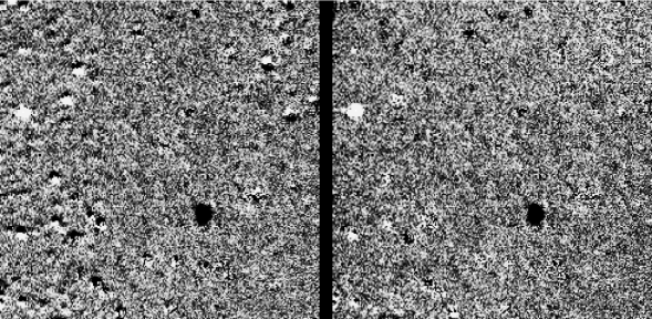
Figure 7: Image subtraction using OGLE II exposures of Galactic Bulge fields. Left is the subtracted image obtained with constant kernel solution. Note the systematic residuals around the bright objects on the left side of the image and in the upper right corner. Note the diseaperance of these pattern in the next image, which has been obtained by fitting the spatial variations of the kernel to order 2. Two variables are present in the field (the bright and dark spots) , and circular areas around these objects had to be excluded for Chi-square evaluation.

Figure 8: Histograms of the normalized deviations in the subtracted images presented in Fig. 7 (OGLE II data). Left is the histogram for constant kernel solution, and right is the histogram for a fit of kernel variation to order 2. The dashed curve is gaussian with $\sigma=1$.

6 Conclusion and summary.

It has been demonstrated that image subtraction with non-constant kernel solution could be achieved in minimum computing time. The cost to perform non-constant solution is only 20 % to 30 % in excess of the constant kernel solution. The ability of the method to deal with PSF variations between the images is demonstrated using Monte-Carlo simulation of stellar fields. It is found that even large relative PSF variations are very well corrected by the method, resulting in a Chi2/Dof very close to 1 in the subtracted image. Non constant kernel solution can also automatically correct for imperfect registration between the images. This possibility is illustrated by generating 2 images with differential rotation with respect to each other. While the systematic pattern due to differential rotation is visible in the subtracted image obtained with constant kernel solution, it disappear completely by fitting the spatial variations of the kernel. To complete the analysis with Monte-Carlo simulation, we tackle the problem of under-sampling by generating 2 very under-sampled images of the same stellar field. A chi-square analysis shows that even in this case an optimal result can be achieved. Finally we apply the method to real astronomical data. It is shown that nearly optimal results can be achieved with non-constant solution, even if the size of the sub-area used for the fit is increased. This result is certainly useful for crowded fields data, but proved to be completely essential in case of fields with low density of high signal to noise objects. A good example is the case of the photometry of the 4 images of the Huchra lens (Wozniak & Alard 1999) To conclude, we can say that new extension of the image subtraction method will certainly prove to be most useful for the supernovae search that are currently undertaken, but may also prove useful for variability search in other galaxies, survey of variables near the core of globular clusters (Olech et al. 1999), and may also become one of the favorite method to analyze microlensing variability in gravitational lens systems.


Software availability:
A set of C programs to perform image subtraction can be obtained on request to C. Alard (alard@iap.fr). Further documentations and C packages will be soon available on a public access Web site.

7 Acknowledgments

It is a pleasure to thank B. Paczyński for his hospitality during my stay in Princeton. I would like to acknowledge support from NSF grant AST 95-30478. I thank B. Paczynski, P. Wozniak, and R. Lupton for many interesting discussions.

References

- [1] Alard, C., & Lupton, R., 1998, ApJ, 503, 325
- [2] Alard, C. and Guibert, J. A&A 1997, 326, 1
- [3] Alcock, C. et al. 1993, Nature, 365, 621
- [4] Aubourg, E. et al. 1993, Nature, 365, 623
- [5] Olech, A., Wozniak, P, Kaluzny, J., & Thompson, I., 1999, in preparation.
- [6] Schechter, P. and Mateo, M. PASP 105, 1342 (1993)
- [7] Tomaney, A. and Crotts, 1996, , A., AJ 112 2872
- [8] Udalski, A. et al. 1994, Acta Astron., 44, 165
- [9] Wozniak, P., 1998, Private communication.
- [10] Wozniak, P., & Alard, C., 1999 in preparation.