Where is the COBE maps’ non-Gaussianity?

Abstract

We review our recent claim that there is evidence of non-Gaussianity in the 4 Year COBE DMR data. We present some new results concerning the effect of the galactic cut upon the non-Gaussian signal. These findings imply a localization of the non-Gaussian signal on the Northern galactic hemisphere.

I Evidence for CMB non-Gaussianity

In a recent paper apjl1 we showed that the 4 Year COBE DMR data exhibits evidence of non Gaussianity at a high confidence level. We made use of statistical tools described in more detail in santa ; bigpaper . Since then our result has been corroborated by two other groups nov ; pando . In this review we revisit our analysis, and the tests to which we have subjected it, including some new results.

In our analysis we propose, and work with, an estimator for the normalized bispectrum, denoted by $I^{3}_{\ell}$. We refer the reader to apjl1 for its definition. We then applied this estimator to the inverse noise variance weighted, average maps of the 53A, 53B, 90A and 90B COBE-DMR channels, with monopole and dipole removed, at resolution 6, in ecliptic pixelization. We use the extended galactic cut of banday97 , and benn96 to remove most of the emission from the plane of the Galaxy. We apply our statistics to the DMR maps before and after correction for the plausible diffuse foreground emission outside the galactic plane as described in kog96b , and COBE .

By means of Monte Carlo simulations we also found the distributions $P_{\ell}(I^{3}_{\ell})$ for what we should have seen assuming a Gaussian signal, which is then processed by the experimental set up associated with DMR. These $P(I^{3}_{\ell})$ were inferred from 25000 realizations (see Fig. 1). The observed $I^{3}_{\ell}$ and the distributions $P_{\ell}(I^{3}_{\ell})$ are plotted in Fig. 1. One immediately notices the presence of a significant deviant.

Figure 1: The vertical thick dashed line represents the value of the observed $I^{3}_{\ell}$. The solid line is the probability distribution function of $I^{3}_{\ell}$ for a Gaussian sky with extended galactic cut and DMR noise.

In order to quantify this deviant we define the goodness of fit statistic

$$X^{2}={1\over N}{\sum_{\ell}X_{\ell}^{2}}={1\over N}{\sum_{\ell}(-2\log P_{\ell}(I^{3}_{\ell})+\beta_{\ell}),}$$ (1)

where the constants $\beta_{\ell}$ are defined so that for each term of the sum $\langle X_{\ell}^{2}\rangle=1$. The definition reduces to the usual chi squared for Gaussian $P_{\ell}$. We build a $X^{2}$ for the COBE-DMR data from the $P_{\ell}(I^{3}_{\ell})$ inferred from Monte Carlo simulations, taking special care with the numerical evaluation of the constants $\beta_{\ell}$. We call this function $X^{2}_{COBE}$. We then find its distribution $F(X^{2}_{COBE})$ from 10000 random realizations. This is very well approximated by a $\chi^{2}$ distribution with 12 degrees of freedom. We then compute $X^{2}_{COBE}$ with the actual observations and find $X^{2}_{COBE}=1.81$. One can compute $P(X^{2}_{COBE}<1.81)=0.98$. Hence, it would appear that we can reject Gaussianity at the $98\%$ confidence level.

II Is it a systematic effect?

We checked that this result could not be due to the following systematics:

1. Foregrounds contamination:

   • Dust (using the DIRBE sky maps and also the Schlegel et al dust model)

   • Synchrotron (with the Haslam template)

   • Foreground corrected maps (effect persists on corrected maps)

2. Noise model:

   • Anisotropic sky coverage

   • Noise correlations between different pixels

   • Analysis of noise templates

3. Galactic cut:

   • Dependence on shape (“custom” versus constant elevation)

   • Dependence on elevation

   • Dependence on monopole and dipole subtraction, before or after the cut, with or with out galaxy.

4. Possible small residual errors in corrections for

   • Spurious offsets induced by the cut.

   • Instrument susceptibility to the Earth magnetic field.

   • Callibration errors .

   • Errors due to incorrect removal of the COBE Doppler and Earth Doppler signals.

   • Errors in correcting for emissions from the Earth, and eclipse effects.

   • Artifacts due to uncertainty in the correction for the correlation created by the low-pass filter on the lock-in amplifiers (LIA) on each radiometer

   • Errors due to emissions from the moon, and the planets.

5. Assumptions in Monte Carlos:

   • Dependence on power spectrum tilt

   • Dependence on smooth versus discontinuous power spectrum

   • Dependence on beam shape

   • Dependence on pixelization.

In fact, the confidence level quoted above reflects the worse line up of systematics. If we try to correct for systematics, in general the confidence level for rejecting Gaussianity is enlarged to beyond 99%, as we describe in more detail in bigpaper

III Where is the non-Gaussianity?

We now concentrate on a subset of tests involving the galactic cut which we applied to our result. Changing the galactic cut affects sample variance besides eliminating possible contaminations from the map. We considered extensive variations of the cut, including additions of polar cap cuts to the extended cut.

Figure 2: The effect of combining the extended cut with polar cap cuts down to $60^{\circ}$ in the North or South hemispheres.

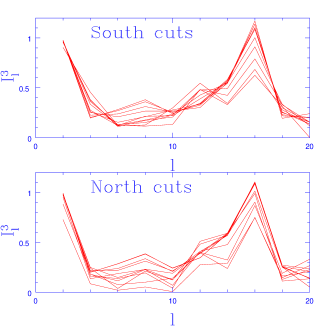
We found that cuts from the pole affect the result more than cuts from the equator. This suggests that the effect may be localized near the Poles. We therefore decided to compare the effect of applying cuts only in the North or South galactic poles. We considered cuts down to $60^{\circ}$ (2668 pixels excluded). We find the curious result that cutting Northern caps is more damaging for the nonGaussian spike than cutting Southern caps (fig. 2). Indeed the first few Southern cap cuts appear to increase the spike.

Non-Gaussianity could in principle be localized in Fourier space without being localized in real space. Examples of such behaviour are given in fermag . We believe that the signal we have found is essentially localized in Fourier space. However the results we have just presented suggest that our signal may indeed be also localised in real space, around the Northern galactic cap.

Acknowledgements JM would like to thank the organizers for an excellent meeting. We thank JNICT, NASA-ADP, NASA-COMBAT, NSF, RS, Starlink, TAC for support.

References

- (1) Ferreira, P. G., Górski, K. M., Magueijo, J. (1998) Ap. J. Lett. 503 L1-L4.
- (2) J. Magueijo, P. Ferreira, K. Gorski, in ”The CMB and the Planck Mission”, proceedings of the UIMP98 meeting held in Santander, Spain, June 22-26, 1998. astro-ph/9810414.
- (3) Magueijo, J., Ferreira, P.G., Górski, K.M., in preparation (1999).
- (4) D. Novikov, H. Feldman, S. Shandarin, astro-ph/9809238.
- (5) J. Pando, D. Valls-Gabaud, L.-. Fang, astro-ph/9810165.
- (6) Banday, A.J., Górski, K.M., Bennett, C.L., Hinshaw, G., Kogut, A., Lineweaver, C., Smoot, G.F., and Tenorio, L. (1997) Ap.J., 475, 393
- (7) Bennet, C.L., Banday, A.J., Górski, K.M., Hinshaw, G., Jackson, P.D., Keegstra, P., Kogut, A., Smoot, G.F., Wilkinson, D.T., Wright, E. L. (1996) Ap. J. 464, 1
- (8) Kogut, A., Banday, A. J., Bennett, C. L., Górski, K. M., Hinshaw, G., Smoot, G. F., Wright, E. L. (1996) Ap. J. 464 L5
- (9) Górski, K. M., Hinshaw, G., Banday, A. J., Bennett, C. L., Wright, E. L., Kogut, A., Smoot, G. F., Lubin, P. (1996) Ap. J. Lett. 464, L11
- (10) P.Ferreira and J.Magueijo, Phys.Rev. D 55 3358 (1997).