Transverse Galaxy Velocities from Multiple Topological Images

Abstract

The study of the kinematics of galaxies within clusters or groups has the limitation that only one of the three velocity components and only two of the three spatial components of a galaxy position in six-dimensional phase space can normally be measured. However, if multiple topological images of a cluster exist, then the radial positions and sky plane mean velocities of galaxies in the cluster may also be measurable from photometry of the two cluster images.

The vector arithmetic and principles of the analysis are presented. These are demonstrated by assuming the suggested topological identification of the clusters RX J1347.5-1145 and CL 09104+4109 to be correct and deducing the sky-plane relative velocity component along the axis common to both images of this would-be single cluster.

Three out of four of the inferred transverse velocities are consistent with those expected in a rich cluster. A control sample of random ‘common’ sky-plane axes, independent of the topological hypothesis, implies that this is not surprising. This shows that while galaxy kinematics are deducible from knowledge of cosmological topology, it is not easy to use them to refute a specific candidate manifold.

1 Introduction

Astronomical observations generally enable three elements of the position of an object in six-dimensional dynamical phase space to be determined: two spatial elements by photometry and one velocity element (radial) by spectroscopy. For extragalactic objects, various techniques enable the cosmological expansion velocity to be approximately subtracted to deduce local (‘peculiar’) radial velocities.

In the study of the dynamics of a galaxy cluster, use of the mean redshift of the cluster implies that these three components are relatively well determined. The other three components remain undetermined, except when occasionally it can be argued that one galaxy is in the foreground of another. To measure the transverse velocity of a galaxy at a redshift $0{.}1<z<1$ to a precision of 100 km s^-1 would require the detection of proper motions of around $0{.}01-0{.}1\mu$arcsec/yr. This is a signal about a thousand times more precise than the noise (uncertainty) in typical VLBI estimates, e.g. of the motion of the Celestial Ephemeris Pole ([][]Souch95), so is not yet practical.

The study of cluster dynamics, therefore, requires simplifying statistical assumptions about the distribution of galaxies in phase space. While this is probably a reasonable approximation for some purposes, measurement of all six elements of kinematical information for each galaxy would obviously enable a much more detailed understanding of the cluster. For example, a net flow of galaxies in a certain three-dimensional direction could be compared to a cooling flow hypothesis or to a study of the merging of sub-structure.

The point of this paper is that measurement of the three missing kinematical parameters for galaxies in the centre of a cluster should be possible in certain cases of multiple topological imaging of clusters. It would be possible to estimate both mean transverse velocities and line-of-sight relative galaxy distances, simply by deep optical imaging.

The reader is first briefly reminded of the nature of multiple topological imaging.

In a standard Friedmann-Lemaître universe of constant curvature, space (or more precisely, a hypersurface at constant cosmological time) is a three-dimensional manifold of which both the curvature and topology need to be measured in order to know its geometry (e.g. [][]deSitt17,Lemait58). The curvature can be described by $\kappa_{0}\equiv\Omega_{0}+\lambda_{0}-1,$ where $\Omega_{0}$ is the density parameter and $\lambda_{0}$ is the dimensionless cosmological constant. Together with the Hubble constant $H_{0}$ these could be referred to collectively as the metric parameters.

The metric parameters are related to local physics and so are, in principle, easy to estimate or constrain by observation of astrophysical objects. In practice, many observational complications arise.

The topology, which could require several parameters to be fully described, is expected only to be related to global physics, so strong theoretical predictions await developments in quantum cosmology (e.g. [][]Hawking84,ZelG84).

So the principle of measuring topological parameters is purely observational, based on the fact that if the ‘size’ of the Universe is smaller than the apparently observable sphere, then photons can travel several times ‘across’ the Universe in less than the age of the Universe. In that case, astrophysical objects would be seen at different celestial positions and different redshifts. The latter is equivalent to different distances and different cosmological epochs. These multiple images are referred to as topological images.

Three-dimensional apparent space interpreted with the assumption of a trivial topology would still be valid, and indeed very useful, to work with for many analyses, even though physically misleading. It would be tiled by ‘copies’ of the Universe, and is termed the ‘covering space’.

Just as for techniques of estimating the metric parameters, observational complications arise in searching for multiple topological images. Indeed, the result of this paper suggests that galaxy kinematics in clusters are not likely to be useful in ruling out identity between two images of clusters.

The word ‘size’ used above needs to be defined more precisely. The size parameters used here are: the ‘out-radius,’ $r_{+},$ which is the radius of the smallest sphere (in the covering space) which totally includes the fundamental polyhedron; and the ‘injectivity radius’, ${r}_{\mbox{\rm\small inj}},$ which is half of the smallest distance from an object to any one of its topological images ([][]Corn98a). The terms ‘injectivity diameter’ for $2{r}_{\mbox{\rm\small inj}}$ and ‘out-diameter’ for $2r_{+}$ are also adopted here.

For reviews on cosmological topology, see [][]LaLu95 (1995; see also [][]Stark98,Lum98,LR99), while recent developments include theory of topology change at the quantum epoch ([][]MadS97,Carl98,Ion98,DowG98,Rosal98,eCF98), ideas for cosmological microwave background (CMB) methods ([][]LevSS98,Corn98b,Weeks98), a review of three-dimensional methods ([][]RB98) and observational analyses which include candidates for the topological parameters ([][]RE97,BPS98). See references in these papers, section 4.3.2 here and [][]Corn98a for CMB-based arguments that ${r}_{\mbox{\rm\small inj}}$ and $r_{+}$ either have or have not been constrained by the COBE satellite.

The basic principle of measuring galaxy transverse velocities is simple. Given the topology parameters to a certain precision, the three-dimensional positions of multiple images of a galaxy known to exist at a certain celestial position and distance (estimated by the redshift) are calculated. If it is the case that several images of the galaxy are expected to be separated by short time intervals, i.e. at similar redshifts, and at widely differing angles, then comparison of optical images should be sufficient to estimate several mean components of the galaxy’s three-dimensional velocity over those time intervals. In the case of two images separated by nearly a right angle, a (near) transverse velocity can be estimated.

The candidate topology suggested by [][]BPS98 (1998, section 4.3) to fit COBE data better than a ‘standard’ CDM model, for $\Omega_{0}=0{.}8,\lambda_{0}=0{.}0$, has a volume larger than that of the observable sphere, so would not imply any multiple images of ordinary astrophysical objects (it would only imply multiple partial images of very large scale temperature fluctuations).

The candidate topological parameters which would be implied by the initial results of the quasar isometry search method of [][]Rouk96 should imply multiple images well within the horizon radius. However, the representations of negatively curved multi-connected manifolds are less simple than those of flat manifolds, and so would not be straightforward to apply.

On the contrary, the candidate topology suggested by [][]RE97, according to which the three rich clusters Coma, RX J1347.5-1145 ([][]Sch96) and CL 09104+4109 ([][]Hall97) would be three topological images of a single cluster, both implies multiple topological images within the horizon and is simple to calculate, since the angle formed by the three (with Coma at the vertex) is close to 90^∘. Moreover, it already includes the topological identification of three known objects of which two are at nearly identical epochs, and close enough that sky survey optical images are readily available.

Hence, the identification of these three clusters by the translations (Coma $\rightarrow$ RX J1347.5-1145) and (Coma $\rightarrow$ CL 09104+4109) in a flat ($\Omega_{0}=1$ or $\Omega_{0}=0{.}2$, and $\Omega_{0}+\lambda_{0}=1$) universe is adopted here for illustration of the derivation of transverse galaxy velocities via multiple topological imaging.

As will be seen below, the results of this calculation show that the converse is not easy: while topology can be used to deduce galaxy kinematics, the expected kinematics of galaxies in clusters do not provide an assumption-free constraint against this cosmological topology candidate in the absence of a full scale photometric and spectroscopic observing programme.

In section 2, the geometry relating the clusters and cluster member galaxies, the selection of galaxies hoped to be cluster members, and the matching of galaxies between two clusters are explained. In section 3, the application to digitised scans of photographic sky survey plates is presented and the resulting transversal velocities are deduced. In section 4, the results are discussed and observational arguments for and against the hypothesised topological identity of the two clusters are listed. A summary is presented in section 5.

For reference, the reader should be reminded that the horizon diameter is $12000$h^-1 Mpc for $\Omega_{0}=1$ ($\lambda_{0}=0$) and $\approx 23400$h^-1 Mpc for $\Omega_{0}=0{.}2$ ($\lambda_{0}=0{.}8$). Except where otherwise stated, distances are quoted as comoving proper distances in the covering space of an $\Omega_{0}=1,\lambda_{0}=0$ universe (hereafter, ‘$\Omega=1$’) or of an $\Omega_{0}=0{.}2,\lambda_{0}=0{.}8$ universe (hereafter, ‘$\Lambda$’) and $h\equiv H_{0}/100$km s^-1 Mpc^-1 is explicitly indicated.

2 Method

The candidate topology of [][]RE97 supposes that in two nearly perpendicular directions, the size of the Universe is $2{r}_{\mbox{\rm\small inj}}\approx(965\pm 5)$h^-1 Mpc for $\Omega=1$ [$2{r}_{\mbox{\rm\small inj}}\approx(1190\pm 10)$h^-1 Mpc for the $\Lambda$ model], and in the third perpendicular direction the size is unknown, i.e. $r_{+}>{r}_{\mbox{\rm\small inj}}$. Because the Universe has no boundaries, photons coming from greater distances in these directions would have in fact already crossed the Universe once or more, so the rich clusters RX J1347.5-1145 and CL 09104+4109 would be images of the Coma cluster seen about $2{.}8$h^-1 Gyr ago for $\Omega=1$ ($3{.}3$h^-1 Gyr for $\Lambda$). These two suggested topological images of Coma are seen at epochs separated by only 35h^-1 Myr for $\Omega=1$ (50h^-1 Myr for $\Lambda$).

If the topological hypothesis were correct, then this small time delay would provide a relatively simple example of observationally deriving transverse galaxy kinematics from identified clusters. Galaxy velocities in clusters are generally of order $\sim 1000$ km s^-1 $\approx 1$kpc Myr^-1 $=1$Mpc Gyr^-1. Comparison of two images of a cluster seen by a separation of 35h^-1 Myr have galaxies which can move by only $\sim 35$h^-1 kpc over this interval, so are unlikely to complete significant fractions of their orbits between the two images. On the contrary, two images of a cluster, even seen from the same direction, but separated by 3h^-1 Gyr, would show a complete scrambling of galaxy sky positions, making identification of corresponding galaxies difficult.

So a criterion for simple determination of galaxy kinematics from topology is that two topological images of a cluster be found which are separated by much less than a dynamical time.

In the case adopted here, this criterion is satisfied, and photographic survey images are available for the two clusters.

2.1 Geometry

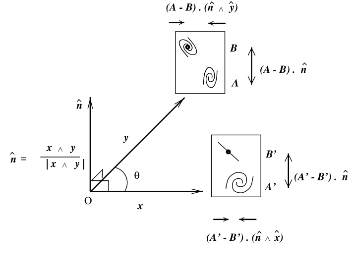
Figure 1: Relative positions of the observer (O) and pairs of galaxy images in two topological images of a cluster of galaxies, for a flat metric, and generators involving only translations (3-D plot). Schematic images of disk galaxies are indicated in order to show how these images would change when seen from different angles. The two clusters are at vector positions $\mn@boldsymbol{x}$ and $\mn@boldsymbol{y}$, separated by some angle $\theta.$ The unit normal to $\mn@boldsymbol{x}$ and $\mn@boldsymbol{y}$ is $\mn@boldsymbol{\hat{n}}\equiv{\mn@boldsymbol{x}\wedge\mn@boldsymbol{y}\over|\mn@boldsymbol{x}\wedge\mn@boldsymbol{y}|}.$ The two galaxies are presumed to be at the mean distance of their parent cluster in each case, at vector positions $\mn@boldsymbol{A}$ and $\mn@boldsymbol{B}$ in one cluster, and at $\mn@boldsymbol{A}\bf{{}^{\prime}}$ and $\mn@boldsymbol{B}\bf{{}^{\prime}}$ in the other cluster. The separations of the two galaxies in the $\mn@boldsymbol{\hat{n}}$ direction, $(\mn@boldsymbol{A}-\mn@boldsymbol{B}).\mn@boldsymbol{\hat{n}}$ and $(\mn@boldsymbol{A}\bf{{}^{\prime}}-\mn@boldsymbol{B}\bf{{}^{\prime}}).\mn@boldsymbol{\hat{n}},$ are measurable from the sky images in both cases, enabling a transverse velocity to be deduced.

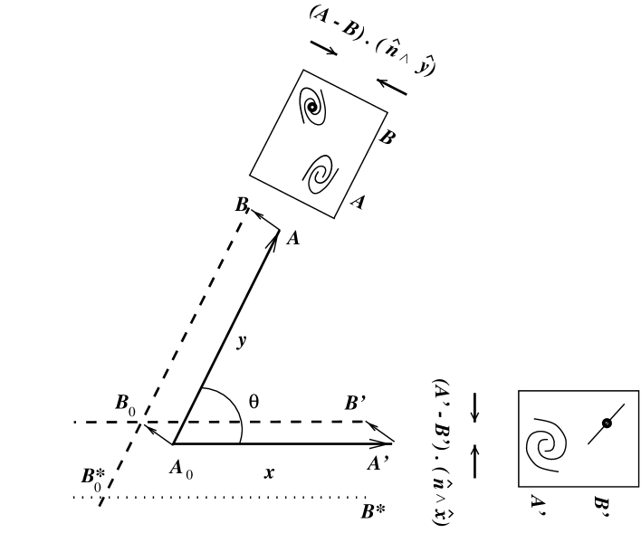
Figure 2: Spatial information available from pairs of galaxy images in two topological images of a cluster, in the $\mn@boldsymbol{x}-\mn@boldsymbol{y}$ plane (cf. Fig. 1). If the epochs of the two topological images are identical, then the two vectors $(\mn@boldsymbol{B}-\mn@boldsymbol{A})$ and $(\mn@boldsymbol{B}\bf{{}^{\prime}}-\mn@boldsymbol{A}\bf{{}^{\prime}})$ are identical, and their projections $(\mn@boldsymbol{B}-\mn@boldsymbol{A}).(\mn@boldsymbol{\hat{n}}\wedge\mn@boldsymbol{\hat{y}})$ and $(\mn@boldsymbol{B}\bf{{}^{\prime}}-\mn@boldsymbol{A}\bf{{}^{\prime}}).(\mn@boldsymbol{\hat{n}}\wedge\mn@boldsymbol{\hat{x}})$ onto the two sky planes, and in the $\mn@boldsymbol{x}-\mn@boldsymbol{y}$ plane, provide two linearly independent components of $(\mn@boldsymbol{B}-\mn@boldsymbol{A})$ in the $\mn@boldsymbol{x}-\mn@boldsymbol{y}$ plane. These are translated to the origin and combined to deduce the separation of $\mn@boldsymbol{A}$ and $\mn@boldsymbol{B}$ in the $\mn@boldsymbol{x}-\mn@boldsymbol{y}$ plane: $(\mn@boldsymbol{B}_{0}-\mn@boldsymbol{A}_{0})$. The point $\mn@boldsymbol{B}^{*}$ is an alternative position for $\mn@boldsymbol{B}\bf{{}^{\prime}},$ showing that a value of $(\mn@boldsymbol{B}^{*}_{0}-\mn@boldsymbol{A}_{0})$ consistent with both sky images can be found even if the topological identification is incorrect. If the topological identification shown here were correct, then $\mn@boldsymbol{B}$ would be slightly in the background of $\mn@boldsymbol{A},$ and $\mn@boldsymbol{B}\bf{{}^{\prime}}$ would be clearly in the foreground of $\mn@boldsymbol{A}\bf{{}^{\prime}}.$

In two images, there are two sky planes each containing two orthogonal directions, making four spatial axes available in total. So, there is at least one spatial parameter which is known in both images. In the case of the hypothesised 3-manifold, in which the generators identifying topological images involve translations only (no rotations or reflections), this spatial parameter can be easily deduced, as is shown in Fig. 1.

For flat multi-connected models in which rotations are involved, or for negatively curved manifolds, the vectors representing the linear transformations from one topological image to another are not generally this simple, so derivation of the parameter in common would be more difficult.

On the other hand, in the case of two images seen in nearly opposite directions in the sky, again for translation-only generators, two spatial directions would be common to both images. This would also apply to images seen in nearly the same direction.

In the case under study here, in which $\theta\sim 90^{\circ},$ the four spatial axes can be chosen such that two are identical. This common axis can be used to determine transverse velocities in one sky direction.

The remaining two axes can be used to fully determine the relative spatial positions of a galaxy pair (Fig. 2), apart from relative movement between the two epochs of observation:

$$(\mn@boldsymbol{B}_{0}-\mn@boldsymbol{A}_{0})=(\mn@boldsymbol{B}-\mn@boldsymbol{A})+(\mn@boldsymbol{v}_{B}-\mn@boldsymbol{v}_{A}).(\mn@boldsymbol{\hat{n}}\wedge\mn@boldsymbol{x})\,\Delta t$$ (1)

to first order in $\Delta t$. This cannot be used as a consistency check for the topological identity of the two images. Any combination of two corresponding galaxy images at close projected distances from their respective cluster centres implies a vector $(B_{0}-A_{0})$ in the $\mn@boldsymbol{x}-\mn@boldsymbol{y}$ plane consistent with both images, even if the galaxy images are not those of a single galaxy seen twice.

The accuracy of the determination of $(\mn@boldsymbol{B}_{0}-\mn@boldsymbol{A}_{0})$ depends on $\theta$. Values of $\theta$ close to zero or $180^{\circ}$ would make the uncertainty in the radial component of $(\mn@boldsymbol{B}_{0}-\mn@boldsymbol{A}_{0})$ high, but at the same lead to the transverse component being nearly similar in the two images, so that both components of the transverse velocity can be calculated, as mentioned above. An angle of $\theta=90^{\circ}$ obviously minimises the uncertainty if measurement of all three spatial separations is desired.

2.2 Galaxy Identification

How can objects in the two topological images of a cluster

• be identified as galaxies which are members of the clusters and

• be matched as identical between the two images?

Determination of cluster membership is not a new question (e.g. [][]KGunn82, section II.b; [][]Sarazin, section II.c). If spectroscopy were available for candidate galaxies in both images, then (a) galaxies which are very likely to be members of a cluster can be decided to reasonable accuracy by a redshift criterion. In that case, it would probably be better to be conservative in the decision on cluster membership, rather than maximally inclusive, in order to avoid wrong matches. That is, galaxies which could ambiguously be interpreted either as high velocity cluster members or as projected foreground/background galaxies would be excluded from the sample. The bias introduced in the distribution of transverse velocities by this conservative inclusion criterion would be of less immediate importance than that which would be introduced by a maximally inclusive criterion.

If deep CCD photometry were available for both images, then a possible technique for (b) would be to rank all galaxies by apparent magnitude and colour and define a difference statistic between the two ranked lists based on the differences in these two parameters. To allow for (i) starbursts, (ii) supernovae, (iii) physical galaxy mergers, (iv) galaxies merged and/or hidden by projection effects and (v) any other effects, perturbations on the lists, in which a small fraction of galaxies can be dropped from either list, or shifted to very different positions, would need to be systematically generated and the difference statistic again calculated.

The difference statistic should also include a parameter representing inconsistency in the appearance of images for individual galaxies. In Fig. 1, it is shown schematically that a disk galaxy seen edge-on at $\mn@boldsymbol{B}\bf{{}^{\prime}}$ may not appear as an edge-on galaxy at $\mn@boldsymbol{B}.$

In fact, if the galaxy at $\mn@boldsymbol{B}\bf{{}^{\prime}}$ is edge-on, i.e. at 90^∘ inclination, and oriented exactly in the $(\mn@boldsymbol{A}\bf{{}^{\prime}}-\mn@boldsymbol{B}\bf{{}^{\prime}}).\mn@boldsymbol{\hat{n}}$ direction, then at $\mn@boldsymbol{B}$ the galaxy should be seen at an inclination of $90^{\circ}-\theta,$ i.e. nearly face-on if $\theta\sim 90^{\circ}.$ On the contrary, if the galaxy at $\mn@boldsymbol{B}\bf{{}^{\prime}}$ is edge-on and oriented perpendicularly to the $(\mn@boldsymbol{A}\bf{{}^{\prime}}-\mn@boldsymbol{B}\bf{{}^{\prime}}).\mn@boldsymbol{\hat{n}}$ direction, then at $\mn@boldsymbol{B}$ the galaxy should also be seen exactly edge-on. For deep photometric CCD images, a parameter for image inconsistency which combines all similar possibilities should be combined with the difference statistic representing magnitude and colour inconsistencies. It would obviously be a much weaker constraint for ellipticals than for disk galaxies.

In order to unambiguously identify galaxies between the two lists, the difference statistic would need to have a sharp minimum at the correct perturbation. This would have to be modelled by starting with a known list of galaxies in a cluster, making reasonable assumptions for (i)-(v), taking into account the time difference between the two images, and calculating the difference statistic for many realisations based on these assumptions.

Since the purpose here is only demonstration, and since the POSS photometry for CL 09104+4109 is not very deep (section 3.1), the criteria adopted here are simply :

• objects with galaxy-like light profiles in the $R$ band, within 400h^-1 kpc of the cluster centre and having $B-R>1{.}5$ are considered to be cluster galaxies (lower limits to $B$ magnitudes are adopted when the galaxy is undetectable in $B$)

• the galaxies are sorted by $R$ and identified between the two images according to their rankings, allowing perturbations for (i)-(v) above only if discussed explicitly.

$R$ band magnitudes are used here since they represent older populations and so are more likely to be stable between the two images.

The brightest galaxies in $R$ in the two images are defined for the present purposes to be the cluster centres, and so considered to be multiple topological images of a single galaxy. In fact, they may not be exactly at the cluster centre (cf. [][]Lazz98), but since it is relative positions which are relevant here, this seems the simplest robust assumption to make. Determination of a ‘true’ centre to the cluster in order to obtain a transversal velocity of the ‘central’ galaxy with respect to the true centre could in principle be carried out by using centres determined by gravitational lensing. For further applications of this method, this would be an option to follow.

In the present case, the lensing analysis of [][]FTys97 seems to show that the brightest galaxy (in $R$) in the central region of RX J1347-1145, labelled galaxy #41^′ (Fig. 6), is close to the gravitational centre of this cluster image. In addition, the brightest galaxy (in $R$) in the central region of CL 09104+4109, labelled galaxy #41 (Fig. 5), should correspond to the radio-quiet quasar which is also a strong IR source ([][]Hall97). This quasar may be related to a cooling flow or a galaxy-galaxy merger, which would suggest that the galaxy should be close to the centre. So the matching of these two galaxies (given the basic hypothesis of identity of the clusters) seems reasonable.

The fact that galaxy #41 lies slightly outside of criterion (a) (since $B-R=1{.}4$) is unsurprising given the presence of the active galactic nucleus (AGN). Strong blue emission from AGN is commonly observed, though the proportions between of light from young, blue, massive main sequence stars and non-stellar astrophysics are unclear. The probability of the phenomenon just starting during the time interval between the emission epochs of the two cluster images is a factor considered in the identification of the two clusters. Since this identification is the assumption made in order to carry out this analysis, the matching of galaxies within the clusters should be made consistently with this assumption.

So, the relative blueness of galaxy #41 should not be used to exclude it, and both criteria (a) and (b) need to be corrected in order to retain consistency.

The correction adopted here is (a) to include this galaxy since it would be more red without a starburst, and (b) if necessary, to slide its ranking in order that it matches the galaxy already labelled #41^′.

3 Results

Red and blue photographic images are available for CL 09104+4109 in the Palomar Optical Sky Survey (POSS) and for RX J1347.5-1145 in the UK Schmidt SRC Southern Sky Survey. Detections of objects in the digitisations of these plates by the APM (Automatic Plate Machine) group at Cambridge, UK, including morphological classifications into galaxy-like or star-like light profiles were obtained. These are displayed in Figs 5 and 6, along with the sky-plane orthonormal vectors discussed in section 2.

Since the POSS data is less deep that that of the UK Schmidt, the images scans of CL 09104+4109 are the limiting factor in comparing the two clusters. This cluster is presented as being at the position of $\mn@boldsymbol{x}$ and RX J1347.5-1145 at the position of $\mn@boldsymbol{y}.$ It should be remembered that the second of these two images is the cosmologically earlier of the two.

3.1 Galaxy Selection

As mentioned above, CL 09104+4109 contains a hyper-luminous IRAS source. Under the assumed hypothesis of topological identity of the two clusters, the event causing this luminosity (e.g. a cooling flow or merger induced star-burst) would have started during the 35h^-1 Myr (50h^-1 Myr) [for $\Omega=1$ ($\Lambda$) respectively] since the emission of the image of RX J1347.5-1145, and if explained by a star-burst would continue for a few hundred Myr longer.

This object is clearly visible as a very bright, moderately red object at the centre of Fig. 5.

Figure 3: $B-R$ colours and $R$ magnitudes of objects detected by APM software in digitised POSS plate at the position of CL 09104+4109 (Fig. 5). Objects having light profiles in both bands characteristic of galaxies, stars or inconsistently as galaxies and stars are indicated as circles, stars and plus symbols respectively. Galaxies undetected in the $B$ ($R$) band are shown as lower (upper) limits by arrows pointing up (down). The numbered objects are those satisfying the cluster membership criteria (section 3.1).

Figure 4: $B-R$ colours and $R$ magnitudes of objects detected by APM software in digitised UK Schmidt survey plate at the position of RX J1347.5-1145 (Fig. 6). Symbols are as for Fig. 3. As discussed in the text, the blue galaxy $34^{\prime}$ is also indicated.

Figs 3 and 4 show the colours and magnitudes of the objects found in the two images, including numeric labels of galaxies as described in the following.

Application of the selection criteria (a) (section 2.2) leads to five galaxies in CL 09104+4109 and four in RX J1347.5-1145. The galaxies are ranked by $R$ according to the suggested option for (b). However, since five galaxies cannot be matched to four, we add to the second list the only other object within 400h^-1 kpc of the centre of RX J1347.5-1145 which is detected as a galaxy in both bands, galaxy #34^′. This galaxy would normally be excluded from the criteria, so to retain physically consistent criteria, it is necessary to suppose that the galaxy was undergoing a starburst at the time of the RX J1347.5-1145 image and that the young, blue stars had left the main sequence by the time of the CL 09104+4109 image, in order that the galaxy was red enough to appear as one of the galaxies already included at this epoch. In that case, the underlying $R$ magnitude of this galaxy without the starburst would be fainter than that measured, so this galaxy is added as the ‘faintest’ galaxy around RX J1347.5-1145 according to the criteria (b).

As discussed above, perturbations in the ordering of the galaxies should, in principle, be considered to take account of the many possibilities of luminosity evolution. A single perturbation in the order is adopted here, i.e. that of supposing galaxy #32 around CL 09104+4109 to be one magnitude brighter than measured. This perturbation is adopted in the numbering of identified galaxies in Figs 3, 4, 5, 6 and 7.

Figure 5: APM scans of red and blue POSS plate photographic images of the core of the cluster CL 09104+4109. East is left and North is up. Size is $4{.}4{{}^{\prime}}{\scriptstyle\times}4{.}4\arcmin.$ Hollow ellipses denote galaxy-like light profiles; solid ellipses star-like profiles. Ellipse sizes denote isophotal solid angles (not brightness). Galaxies passing the selection criteria discussed in section 3.1 are numbered. The vector shown in bold is $\mn@boldsymbol{\hat{n}},$ the normal common to both the lines-of-sight $\mn@boldsymbol{x}$ (from the observer to this cluster) and $\mn@boldsymbol{y}$ (from the observer to RX J1347.5-1145). The other vector shown is $\mn@boldsymbol{\hat{n}}.\mn@boldsymbol{\hat{x}}.$ The two vectors are shown with modulus $1{.}5{{}^{\prime}}$ $=438$h^-1 kpc. Galaxies 34, 33 and 38 are not detected in the $B$ band. The cluster is at redshift $z=0{.}442$ ([][]Hall97).

Figure 6: Galaxies in the core of the cluster RX J1347.5-1145, from UK Schmidt survey plate scans. Axes and symbols are as for Fig. 5 except that primed numbers indicate galaxies which would be identified with those in Fig. 5, and the secondary vector is $\mn@boldsymbol{\hat{n}}.\mn@boldsymbol{\hat{y}}.$ The vector shown in bold is identical, in three-dimensional space, in both figures. The two vectors are shown with modulus $1{.}5{{}^{\prime}}$ $=444$h^-1 kpc. Galaxy 38^′ is not detected in the $B$ band. The cluster is at redshift $z=0{.}451$ ([][]Sch96), i.e. the image was emitted at a slightly earlier epoch than that of CL 09104+4109.

The image scans, shown in Figs 5 and 6, enable relative galaxy positions in the direction of the mutual normal $\mn@boldsymbol{\hat{n}}$ to be judged by eye.

Figure 7: Resultant galaxy transverse velocities implied by topological identity of the two clusters via a translation, shown in  km s^-1 against the implied ‘two-dimensional’ radial distances, in h^-1 kpc, from the galaxy close to the centre of the cluster. The radial distances are defined as ${r}_{\mbox{\rm\small 2D}}\equiv|\;[(A^{\prime}-B^{\prime}).(\mn@boldsymbol{\hat{n}}\wedge\mn@boldsymbol{\hat{x}})]\,(\mn@boldsymbol{\hat{n}}\wedge\mn@boldsymbol{\hat{x}})+[(A^{\prime}-B^{\prime}).(\mn@boldsymbol{\hat{n}}\wedge\mn@boldsymbol{\hat{y}})]\,(\mn@boldsymbol{\hat{n}}\wedge\mn@boldsymbol{\hat{y}})\;|$ $\equiv\sqrt{r^{2}-r_{\perp}^{2}},$ where $r$ and $r_{\perp}$ are defined as in Table 1. That is, ${r}_{\mbox{\rm\small 2D}}$ is the radial distance in the plane perpendicular to that of the velocity component measured. Solid circles indicate the implied velocities for the hypothesised common axis, other symbols indicate velocities calculated for random orientations of $\mn@boldsymbol{\hat{n}}$ in the two sky planes. The dotted lines indicate $\pm 3$ $\sigma_{v},$ where $\sigma_{v}$ is a smooth fit to the velocity dispersions measured in the Coma cluster by [][]KGunn82.

Table 1: Properties of matched galaxies: identity number; celestial positions in images (1) CL 09104+4109 and (2) RX J1347.5-1145; apparent magnitude $R_{2}$ and the colour $C_{2}\equiv(B-R)_{2}$ in (2) and their increments $\Delta R\equiv R_{1}-R_{2},$ $\Delta C\equiv(B-R)_{1}-(B-R)_{2}$ (in mag); transverse velocity component $v_{\perp}$ in direction $\mn@boldsymbol{\hat{n}}$ (in  km s^-1 ); average distance $r_{\perp}$ from centre in direction $\mn@boldsymbol{\hat{n}}$; distances in background of centre $r_{1}$ and $r_{2}$ in images (1) and (2) respectively; three-dimensional distance $r$from centre (in h^-1 kpc). Notes: ^alower limit to $(B-R)_{2}$; ^bnot detected in $B$ in either image.

$$\begin{array}[]{r cccc cccc rrrrr}\hline\cr\mbox{\rule[-1.29167pt]{0.0pt}{8.61108pt}}\#&\alpha_{1}&\delta_{1}&\alpha_{2}&\delta_{2}&R_{2}&C_{2}&\Delta R&\Delta C&v_{\perp}&r_{\perp}&r_{1}&r_{2}&r\\ \hline\cr\mbox{\rule[0.0pt]{0.0pt}{8.61108pt}}41&9^{h}13^{m}45.5^{s}&40^{\circ}56{{}^{\prime}}27.8{{}^{\prime\prime}}&13^{h}47^{m}30.6^{s}&-11^{\circ}45{{}^{\prime}}9.8{{}^{\prime\prime}}&19.0&1.6&-1.8&-0.2&0&0&0&0&0\\ \mbox{\rule[0.0pt]{0.0pt}{8.61108pt}}32&9^{h}13^{m}43.9^{s}&40^{\circ}56{{}^{\prime}}54.4{{}^{\prime\prime}}&13^{h}47^{m}31.9^{s}&-11^{\circ}45{{}^{\prime}}11.1{{}^{\prime\prime}}&19.5&2.4&0.3&-0.6&752&72&-68&-130&157\\ \mbox{\rule[0.0pt]{0.0pt}{8.61108pt}}33&9^{h}13^{m}39.7^{s}&40^{\circ}56{{}^{\prime}}51.2{{}^{\prime\prime}}&13^{h}47^{m}27.8^{s}&-11^{\circ}45{{}^{\prime}}2.5{{}^{\prime\prime}}&19.8&1.6&-0.9&<1.2&2866&-70&169&-335&405\\ \mbox{\rule[0.0pt]{0.0pt}{8.61108pt}}38&9^{h}13^{m}41.0^{s}&40^{\circ}56{{}^{\prime}}34.2{{}^{\prime\prime}}&13^{h}47^{m}28.0^{s}&-11^{\circ}45{{}^{\prime}}52.7{{}^{\prime\prime}}&20.1&2.7^{a}&-0.9&-^{b}&6330&-176&-15&-235&294\\ \mbox{\rule[0.0pt]{0.0pt}{8.61108pt}}34&9^{h}13^{m}48.2^{s}&40^{\circ}56{{}^{\prime}}44.0{{}^{\prime\prime}}&13^{h}47^{m}34.2^{s}&-11^{\circ}45{{}^{\prime}}20.5{{}^{\prime\prime}}&19.8&0.4&-0.3&<1.8&-461&140&-221&107&296\\ \hline\cr\end{array}$$

3.2 Transverse velocities

Fig. 7 shows the resultant transverse velocities, plotted against a ‘two-dimensional’ radial distance ${r}_{\mbox{\rm\small 2D}}$ (see caption for definition), in order to make comparison with other observational analyses as direct as possible.

For comparison, ten random axes in the two sky planes are generated and transverse velocities calculated just as for the hypothesised axis $\mn@boldsymbol{\hat{n}}$ which is consistent between the two images.

Both the hypothesised axis and the control axes give at least one transverse velocity which is obviously too high for a cluster member in each case. The results for the random axes shown by an ‘x’ and by a triangle are the most similar to those for the hypothesised axis.

In the case of the hypothesised axis, it is not possible to interpret the high velocity as indicating a galaxy which is not a cluster member. It would indicate that the two matched galaxy images are not of the same galaxy, and that at least one of these is probably a foreground or background interloper. For galaxies seen in the lines-of-sight to two topologically identical clusters, only those close to the respective cluster distances would be common to both lines-of-sight (apart from rare special cases). Interlopers would cause false matches, and in the cases where the inferred velocity is unreasonably high, this would only indicate rejection of the galaxy-galaxy match, not a velocity of the interloper.

Table 1 lists not only the transverse velocities but also full three-dimensional information on the spatial displacements of galaxies from the cluster centre, as derived from equation 1. Since $\theta\approx 90^{\circ}$ in the case studied here, the three components are approximately orthogonal and $r^{2}\approx r_{\perp}^{2}+r_{1}^{2}+r_{2}^{2},$ but this would not be the case in general. For example, for a topological image pair separated by 45^∘the approximation would not hold.

If spectroscopic information were available for galaxies in the two images, then the remaining two velocity components would also be measurable here.

The parameter $r_{i}$ (for the ${i}^{\mbox{\rm\small th}}$ of the two images) indicates whether galaxies are in the foreground ($r_{i}<0$) or the background ($r_{i}>0$) of the cluster centre.

3.3 Uncertainties

The positions generated by the APM are considered accurate to about $0{.}5$^′′, the colours to about $\pm 0{.}2$mag and the magnitude zero-points to about $0{.}25$mag (on-line facility). If we consider the uncertainties in the redshifts of the two cluster images to be $\Delta(z)\sim 0{.}001,$ i.e. 300 km s^-1 , then the statistical errors in the perpendicular velocities are about 17%, dominated by the uncertainty in the time interval implied by the uncertainties in the redshifts, while the foreground and background offsets of galaxies are uncertain by 4h^-1 kpc.

Since the uncertainty due to that in the time interval is essentially a fixed numerical value, it would become fractionally smaller for an image pair separated by a larger time interval, making the transverse velocity uncertainties smaller. However, a larger time interval would also allow the possibility for galaxies to traverse larger fractions of their orbits, so that the mean transversal velocity would become a less useful quantity (e.g. a mean transversal, or radial, velocity over exactly one orbit is zero).

Whether the real Universe gives us a choice of enough cluster pairs such that we have the luxury of choosing which pairs are best to be analysed remains to be seen. The candidate examined here is all that is available until further topological image pairs of clusters are proposed.

Systematic errors (apart from wrong matching of cluster pairs by cosmological topology) are most likely to be present as the wrong matching of galaxy image pairs. Wrong matches can be generated either by the uncertainties in the zero-points and magnitudes of the galaxies which allow errors in the ranking procedure or by non-cluster members which are included in the list for either cluster image.

In a full scale observing program to implement the method presented here, CCD photometry and spectroscopy should increase the accuracy with respect to all the different sources of uncertainties.

4 Discussion

Given the assumption of topological identity of two clusters under a translation, it has been seen how galaxy transverse velocities can be deduced. Obviously, once (or if) the topology of the Universe is detected by techniques such as the CMB technique of [][]Corn98b or the three-dimensional techniques of [][]LLL96 or of [][]Rouk96, deep photometry of clusters would enable methods such as those presented here to be applied in much more detail to make a systematic study of transverse galaxy velocities — and full six-parameter kinematical information — in a cluster.

In the present study, simple physical constraints based on sky-survey image data result in quite reasonable transverse velocities for the galaxies in the supposedly single cluster RX J1347.5-1145/CL 09104+4109, apart from that of galaxy #38. This latter ‘galaxy’ would be best be explained as a wrong galaxy-galaxy match, e.g. due to at least one of the galaxies being an interloper.

4.1 Photometric Evolution

Are the photometric properties of the matched galaxies consistent with ordinary stellar evolution? The changes in apparent magnitude and colour are listed in Table 1 (expressed as the change in each parameter as cosmological time increases).

Apparent magnitude is related to absolute magnitude by the luminosity distance, the K-correction (redshift effects for a galaxy of non-evolving stellar population) and the E-correction (evolutionary effect at a single redshift). The difference in luminosity distances of the two clusters implies only $0{.}05$ brightening over the time interval and the difference in K-corrections should also be small.

If uncertainties $\delta(R)\approx\delta(B)$ are adopted, then the uncertainties for the photometry as cited in section 3.3 imply $\delta(R)\approx 0{.}14$mag. Combining this with the zero-point uncertainty gives $\delta(\Delta R)=0{.}41.$

Apart from galaxy #41, which we know to be a strong IR source and therefore exceptional, and galaxy #38, which should be rejected on the ground of its high velocity, the remaining three galaxies are in fact consistent with no $R$ band evolution to $0{.}7\sigma$ (galaxies #32 and #34) and to $2{.}2\sigma$ (galaxy #33). The latter galaxy would marginally have to brighten over the time interval.

Because of the faintness of the galaxies, several are not detected in $B$, particularly in the POSS plate, but the lower limits in $(B-R)$ are nevertheless useful for constraining colour evolution.

The uncertainty in the colour change is $\delta(\Delta C)=0{.}28$ (colour change is more precise than magnitude change due to the zeropoint uncertainties in the magnitudes). This implies inconsistency with no colour evolution at at least $4\sigma$ and $6\sigma$ for galaxies #33 and #34 respectively, in the sense that these galaxies become at least $1{.}2\pm 0{.}3$mag and $1{.}8\pm 0{.}3$mag more red, respectively, over $35\pm 5$h^-1 Myr ($\Omega=1$).

Both of these galaxies’ colours in the earlier of the two images, i.e. $C_{2},$ are relatively blue. The normal explanation for this is that they are seen at the end of a starburst.

How rapidly can a starburst galaxy redden following the end of a starburst? As long as at least a few percent of the mass of a galaxy is involved in the starburst, the newly formed stars still dominate the optical spectrum up to $\sim 100$Myr after the starburst has terminated, so it is sufficient to consider the reddening of a stellar population created in an instantaneous starburst. For example, see Fig. 4 of [][]BC93.

Estimation from this figure indicates that (for a Salpeter initial mass function, IMF), between 1 and 10 Myr from the occurrence of an instantaneous starburst, the $(B-R)$ colour can redden by about $1{.}4$mag. On the other hand, between 1 and 10 Myr from the onset of a constant star formation rate (SFR) period, the $(B-R)$ colour can redden by about $0{.}6$mag. At the same time, the $R$ band magnitudes should brighten according to $\Delta R=-1{.}1$ and $\Delta R=-3{.}6$ respectively.

Given the uncertainties these values provide a fair guide for the time interval here of $35\pm 5$h^-1 Myr.

This would make galaxies #33 and #34 consistent with the endpoints of starbursts to $0{.}7\sigma$ and $1{.}4\sigma$ respectively, by their colours, and to $0{.}5\sigma$ and $2\sigma$ respectively, in their $\Delta R$ values.

If reddening by dust were taken into account, many other possibilities would be possible.

The chance of seeing the end or the beginning of a starburst depends on whether the starbursts frequently seen in cluster galaxies at redshifts $z\,\lower 2.58334pt\hbox{$\buildrel>\over{\sim}$}\,0{.}3$ ([][]BO78,ODB97) are continuous and smooth or are composed of many short star formation periods. Relatively many short bursts would be required for the probability of seeing the end or the begininning of a starburst to be significant.

In the case of a full observing program including spectrophotometry, detailed studies should enable stellar population evolution of individual galaxies to become a check on the consistency with the original hypothesis, but this is not the case here.

4.2 Further Work

The determination of cluster membership and constraints on stellar population evolution would obviously benefit from both deep photometry and spectroscopy.

In fact, the consistency of the kinematics and photometry for the assumed topological image pair of clusters indicate that both types of observations would be necessary if this method were to be considered a means of refuting a cosmo-topological hypothesis.

This would not necessarily be sufficient, however. Higher numbers of fainter galaxies would enable more possible matches. Historical experience with measurement of other cosmological parameters suggests that these parameters are often more useful as inputs than as outputs of small-scale galaxy studies, so the topological parameters do not seem to provide an exception.

So, although a full scale observing programme on these two cluster images could be motivated by the desire to investigate how well this method can exclude a candidate pair of topologically imaged clusters, it could be more safely motivated by independent evidence strengthening the candidate match.

4.3 Arguments For and Against the Topological Identity

For completeness, various arguments for and against the hypothesised image pair, and observational predictions based on the same hypothesis, are resumed below. The reader is reminded that the two clusters would be also physically identified with the Coma cluster.

4.3.1 Likelihood of Finding Near Right-Angled Configurations

This geometrical configuration in the covering space is one which has already been searched for among other objects (e.g. quasars, [][]Fag87), and was found among a very small number of objects by [][]RE97. An a posteriori calculation of the probability of finding this configuration, particularly given the subjective selection of the very small list of bright clusters, would be difficult to do objectively.

The striking nature of the configuration would not be a strong argument alone, but the history of literature on hypertorus models (section 4.3.2) and the simplicity of the configuration make it good as a working hypothesis, to see how tightly methods which attempt to constrain topology can really work if considered with the same care as methods to constrain the metric parameters, $\Omega_{0},H_{0}$ and $\lambda_{0}.$

4.3.2 CMB Analyses

To test the consistency of a candidate 3-manifold with CMB data would require application of the ‘identified circles’ principle ([][]Corn98b).

The identified circles principle is simply the property that the sets of multiply imaged points on the SLS would form pairs of identified circles, if non-trivial topology were detectable. If locally anisotropic radiation from the SLS (e.g. the Doppler effect) and foregrounds are insignificant, then any specific candidate can therefore be falsified by showing that the temperature fluctuations running around hypothetically identified circles are significantly different. This is independent from assumptions regarding the statistics of density perturbations, but does depend on the assumption that the radiation is locally isotropic.

Because of the poor signal-to-noise ratio and resolution, this has not yet been systematically applied to COBE data to constrain multi-connected universe models. It is intended to be applied to observational data from the MAP and Planck satellites ([][]Corn98a).

However, in spite of the poor signal-to-noise and resolution, several CMB analyses based on COBE data have been attempted for hypertoroidal universes (see [][]Corn98a and references therein), by (i) modelling individual 3-manifolds and (ii) assuming properties of the perturbation spectrum — Gaussian distributions in the real and imaginary parts of the amplitudes of density perturbations and a power spectrum of shape $P(k)\propto k^{1}$. The authors claim that the COBE data are inconsistent with hypertoroidal universes of $2{r}_{\mbox{\rm\small inj}}\,\lower 2.58334pt\hbox{$\buildrel<\over{\sim}$}\,R_{H}/2$. Since in the present case $2{r}_{\mbox{\rm\small inj}}\approx 0{.}16R_{H}$ for $\Omega=1$ (for $\Lambda$ we have $2{r}_{\mbox{\rm\small inj}}\approx 0{.}10R_{H}$), this would seem to provide evidence against the hypothesised topological identity adopted for the illustration in this paper.

However, these analyses consist more of a test of the assumptions (ii) on large scales rather than of the topology of space. They do not refute the hypertoroidal models tested: this would require an application of the identified circles principle.

The theoretical motivation for (ii) is unlikely to be valid at scales approaching ${r}_{\mbox{\rm\small inj}}$ and $r_{+}$. That is, either for a hyperbolic or for a flat, $\lambda_{0}\sim 0.7$ metric to be presently observable, inflation needs some degree of fine-tuning (which can partly be provided by the ergodicity of geodesics in the former case, [][]Corn96). Since curvature or $\lambda_{0}>0$ must remain “uninflated” in the sense of being observable at the present epoch in these cases, it is unclear why perturbations on the scale of $R_{C}\sim R_{H}$ should necessarily be “inflated” in the sense of exactly satisfying the assumptions on the power spectrum. Moreover, even for other choices of metric, if the Universe has observable non-trivial topology, then scales approaching ${r}_{\mbox{\rm\small inj}}$ and $r_{+}$ need not necessarily be “inflated” either.

The observational motivation for (ii) is equally lacking for tests of non-trivial topology. The only observational justification of these properties on large scales is COBE data, which is analysed assuming trivial topology. This cannot be used to test non-trivial topology.

So the statistical confidence levels quoted for these papers rejecting hypertoroidal universes should be interpreted as statements about theoretical random realisations where the properties of large length scale ($r=2\pi/k\sim{r}_{\mbox{\rm\small inj}}<r_{+}$) density perturbations are assumed to be unaffected by the finiteness of the Universe apart from a sharp cutoff. (Note also that some authors find evidence for non-Gaussian distributions: [][]Ferr98,Pando98).

Nevertheless, even if it is assumed that the perturbation properties satisfy “inflationary” conditions at the topology length scales, if one disregards the other simplifications of the physics at the SLS in the standard COBE analyses, the possible contamination by foregrounds, and the poor signal-to-noise and resolution ($\sim$ 10^∘) of the COBE maps, the present hypothesis would still not be excluded. The $T^{2}$ candidate suggested has ${r}_{\mbox{\rm\small inj}}\ll R_{H}$ but $r_{+}\gg R_{H}$. Since most work deals with $r_{+},$ it does not apply in the present case.

Specifically, the orientation of the long (unconstrained) axis of the toroidal universe hypothesised here is about 23^∘ from the galactic plane, so that the smallest cross-sections of copies of the fundamental polyhedron with the surface of last scattering (SLS) are mostly obscured by or at least affected by galactic contamination. The most visible cross-sections are large. This would generate the large scale power, which should, in some average sense across different realisations of the universe, cut off above a scale related to $r_{+}.$

In the work most relevant to the present case, [][]deOliv96 present an interesting method, where ${r}_{\mbox{\rm\small inj}}<R_{H}\ll r_{+}$ hypertori are considered. Fig. 1 (top right) of [][]deOliv96 should be similar to a CMB map expected for the $T^{2}$ candidate used here, though it should also have the plane of the Galaxy removed, the long axis oriented at about 23^∘ from the galactic plane rather than 90^∘, and a ‘cell size’ smaller by a factor of two. Fig. 3 of [][]deOliv96 would imply that our $T^{2}$ candidate is rejected at more than $2\sigma$ by the authors’ $S_{0}$ statistic, so this is potentially interesting.

However, apart from the fact that the $2\sigma$ rejection is a statement about the statistics of the perturbation simulations rather than about observational inconsistency, the fact that the method involves detecting symmetry implies that it is specially sensitive to any asymmetries in the noise contributions. Galactic foregrounds are far from being isotropic. So, a parameter representing symmetry in the CMB from the component at the SLS, due to the $T^{2}$ topology, strongly risks damping by asymmetry from foregrounds.

If [][]deOliv96’s method were to be applied more thoroughly, in order to provide more serious constraints, it would be necessary to consider (i) a wider range of assumptions on the fluctuation statistics, (ii) the integrated Sachs-Wolfe effect and the Doppler effect, (iii) correlations in the galactic and extragalactic foregrounds, and (iv) removal of the contaminated areas suggested by [][]CaySm95.

4.3.3 Coincidences of Large Scale Structure

[][]RE97 noted that with the correct topological hypothesis, the distribution of large scale structure in walls, bubbles and filaments at scales around $50-150$h^-1 Mpc (e.g. [][]deLapp86,GH89,daCosta93,Deng96,Einasto97), which quasars can be expected to trace, should enable significant correlations to be measured. No significant correlation was found with the parameters published in that paper.

Since the auto-correlation function of galaxies at $2\,\lower 2.58334pt\hbox{$\buildrel<\over{\sim}$}\,z\,\lower 2.58334pt\hbox{$\buildrel<\over{\sim}$}\,3$ (where the majority of observed quasars lie), may cover a range of amplitudes overlapping the present values (e.g. [][]RVMB98 at small separations), this is potentially a good method of refuting or strengthening a candidate for the 3-manifold of the Universe. The method is in fact equivalent to that of [][]LLL96, except that (a) individual objects are replaced by ‘pixels’ of filaments and walls in large scale structure of thickness not much less than 10% of their separations, and (b) the ‘pixels’ are sampled very sparsely and non-uniformly, so that the spikes expected would be much less strong than in the plots of these authors.

Indeed, the $\sim 8000$ quasars presently identified with $z>1$ are both unevenly distributed and rare, with a mean separation of $\,\lower 2.58334pt\hbox{$\buildrel>\over{\sim}$}\,100$h^-1 Mpc. This implies typically one or a few quasars per entire ‘unit’ of large scale structure, so that pairs of quasars seen in topologically identified ‘pixels’ would be rare.

Other factors are (a) it could be the case that the angles of the fundamental cube are not perfect right angles, particularly since the identity between the three clusters is not exactly a right angle, and that the sides are of slightly unequal lengths; and (b) the test should also be performed for a range of $\lambda_{0}$ values giving flat metrics. It would be sufficient to be one degree in error in the orientation or to have $\lambda_{0}$ mis-estimated by $0{.}02$ to have a transversal error of $\sim 60$ h^-1 Mpc at typical quasar distances of $z\sim 3.$ This error is at the same scale as that of large scale structure, so would be likely to swamp any genuine signal.

This technique would therefore require at least an order of magnitude more $z\,\lower 2.58334pt\hbox{$\buildrel>\over{\sim}$}\,1$ objects and detailed consideration of sources of uncertainty in order to significantly refute candidates for the topology of the Universe, but in principle could be powerful.

4.3.4 Mass Estimates

The total masses are identical within the uncertainties. [][]Briel92 ROSAT estimates for Coma are $(4-10){\scriptstyle\times}10^{14}M_{\odot}$ to $1h_{50}^{-1}$ Mpc and $(10-20){\scriptstyle\times}10^{14}M_{\odot}$ to $3h_{50}^{-1}$ Mpc; [][]Sch96 give $5{.}8{\scriptstyle\times}10^{14}M_{\odot}$ and $17{\scriptstyle\times}10^{14}M_{\odot}$ for RX J1347.5-1145 to the same radii respectively; and the gas fraction to a large radius appears lower in Coma, but consistent within the uncertainty.

From gravitational lensing data, [][]FTys97 infer the mass of RX J1347.5-1145 as $(11\pm 4){\scriptstyle\times}10^{14}M_{\odot}$ within the central $2h_{50}^{-1}$ Mpc, consistent with the above estimates for a simple $M\propto R$ profile.

4.3.5 X-ray Fluxes

The X-ray flux and core ($r<500h_{50}^{-1}$ kpc) surface brightness of RX J1347.5-1145 are considerably higher than those of Coma, e.g. $L_{X}(0{.}1-2{.}4$ keV$)$ of RX J1347.5-1145 is about ten times as high as that of Coma . Taking into account the X-ray ‘K-correction’ would only make the intrinsic $L_{X}(0{.}1-2{.}4$ keV$)$ a small factor smaller. For RX J1347.5-1145 and Coma to be images of one another, a large reduction in emission due to the removal of a cooling flow, possibly due to the merger between sub-clusters, would have to have occurred.

In fact, Coma does not have a cooling flow, and [][]Biv96 argue that Coma has had a recent merger of two subclusters (and is ongoing a merger with another subcluster), so any cooling flows are very likely to have been disrupted. Models by [][]AllFab98 and [][]Peres98 show that up to 70% of a cluster’s luminosity can be due to the cooling flow, so once this is removed, the luminosity of RX J1347.5-1145/CL 09104+4109 could drop to close to that of Coma. In addition, Table 1 and Fig. 2 of ([][]AllFab98) show that bolometric luminosity estimates for these two images (which are at nearly the same redshift, so have little relative K-correction) agree within $1{.}4\sigma.$

4.3.6 Coincidence of Seeing Galaxy #41 Just Before and During a Highly Luminous IR Phase

As mentioned above, for RX J1347.5-1145 and CL 09104+4109 to be identical, the quasar (lying in the galaxy labelled here as #41) seen only in the latter would have to have started during the time interval separating the two images.

The part due to stellar luminosity, mostly reradiated in the far-IR by dust but with some blue light escaping, would have a time scale for the massive stars to leave the main sequence of $\sim 100$ Myr. The time scale for the duration of this episode of AGN activity, if due to the merger of typical large galaxies of $10^{12}M_{\odot},$ would be about $200$ Myr, while [][]Cavpad88 estimate that quasar lifetimes are likely to be at most about a 1 Gyr. So if RX J1347.5-1145 and CL 09104+4109 are indeed the same cluster, it would be about a 10% coincidence that we happen to see one image just before the event started and one during the event. This is not a strong argument against identity.

The time difference of about $3$h^-1 Gyr between these two images and that of Coma implies that the AGN would most probably have finished by the epoch of Coma, so would provide no constraint at all, whether seen or not in the latter.

4.4 Observational Predictions of the Topological Identity

4.4.1 Further Topological Images

The hypothesised generators imply other images of the would-be single cluster. The most easily observable of these, at redshifts low enough that the cluster is known to already exist, and at which uncertainty in the metric parameters does not imply too much uncertainty in predicted positions, would be those at the antipodes (Coma centred) to RX J1347-1145 and CL 09104+4109.

These positions are

$${\mn@boldsymbol{r}}_{\mbox{\rm\small Coma}}- (\mn@boldsymbol{\hat{y}}-{\mn@boldsymbol{r}}_{\mbox{\rm\small Coma}})=$$

$$(0{.}40\pm 0{.}01, 20^{h}40^{m}\pm 6^{m},-40^{\circ}40{{}^{\prime}}\pm 20{{}^{\prime}})$$

$${\mn@boldsymbol{r}}_{\mbox{\rm\small Coma}}- (\mn@boldsymbol{\hat{x}}-{\mn@boldsymbol{r}}_{\mbox{\rm\small Coma}})=$$

$$(0{.}40\pm 0{.}01, 01^{h}57^{m}\pm 4^{m},+17^{\circ}25{{}^{\prime}}\pm 70{{}^{\prime}})$$

where $\mn@boldsymbol{\hat{x}}$ and $\mn@boldsymbol{\hat{y}}$ are as above, ${\mn@boldsymbol{r}}_{\mbox{\rm\small Coma}}$ is the position of Coma, and the values are $(z,\alpha,\delta)$ (J2000.0).

RX J203150.4-403656 is a candidate for the former image. Spectroscopy to determine its redshift and an optical (or X-ray) search for a cluster within $\,\lower 2.58334pt\hbox{$\buildrel<\over{\sim}$}\,1{.}5^{\circ}$ of ($1^{h}57^{m},+17{.}5^{\circ}$) and within $\delta(z)\,\lower 2.58334pt\hbox{$\buildrel<\over{\sim}$}\,0{.}01$ of $z=0{.}40$ would be needed to either increase the precision of or rule out variants on the candidate manifold suggested. In the latter case, lack of deep ROSAT exposure and a foreground Abell cluster make the search for a cluster in this region difficult.

4.4.2 Infall of Sub-cluster(s)

For the cooling flow in RX J1347.5-1145 to be disrupted by subcluster merging, and for subcluster merging to continue by the time we observe Coma, the infalling sub-cluster(s) should be visible close to RX J1347.5-1145. ROSAT pointed observations or deep optical imaging over a 20–30^′ field around the cluster should be sufficient to detect the subclusters if their relative transversal velocities are no more than around 1500 km s^-1 .

5 Conclusion

The techniques of deducing galaxy transverse velocities and foreground/background spatial offsets relative to a cluster ‘central’ galaxy, in the case that a non-trivial topology of the Universe is known and has $2{r}_{\mbox{\rm\small inj}}\ll 2R_{H},$ have been presented.

In the case of a 3-manifold for which there are two topological images of a given galaxy cluster

• only separated by a translation (no rotation nor reflection) and

• for which the time interval between the two images is relatively short (much less than a dynamical time of the cluster);

then

• there is at least one common axis to the two sky planes, which is simply given by the normal to the two vectors pointing to the two images;

• simple criteria can be chosen to match galaxies between the two images;

• the shifts of corresponding galaxies relative to the cluster centre over the time interval imply transverse velocities and

• if the image separation is closer to 90^∘ than to 0^∘ or 180^∘, then the remaining sky offset components can be used to deduce the other components of the full three-dimensional relative positions of the galaxies. Spectroscopy would enable the remaining two velocity components to be estimated.

For a 3-manifold for which two topological images are separated by a less simple isometry, the present calculation would have to be generalised.

For the hypothesised identification of the rich clusters RX J1347.5-1145 and CL 09104+4109, scans of the UK SRC Schmidt Southern Sky Survey and the Palomar Optical Sky Survey digitised plates were subjected to a simple version of the criteria suggested for matching galaxies between the two images.

The common sky-plane axes, transverse velocities, spatial background/foreground offsets and photometric evolution of matched galaxies were calculated. Only one of the transverse velocities is rejected on the grounds of being much higher than the velocity dispersion of the would-be single cluster. A control sample of randomly orientated axes gives about a 20% chance of inferring a similarly reasonable set of velocities. The photometric evolution is consistent with the galaxy matches, so is not useful (in this case at least) for refuting the original hypothesis.

This method shows how galaxy transverse velocities can be estimated, given a knowledge of multiply topologically imaged clusters by other means. Given the ease of finding reasonable velocities for a 3-manifold candidate which is in no way anything more than a candidate, it is clear that this method is not optimal for the inverse process, i.e. for refuting a candidate for the topology of the Universe. It is possible that deep photometry and spectroscopy could enable such a refutation, though this would at a minimum require a full scale observing programme.

Regarding the hypothesis adopted, the reader is reminded that observations to determine the redshift of RX J203150.4-403656 and to search for a cluster within $\,\lower 2.58334pt\hbox{$\buildrel<\over{\sim}$}\,1{.}5^{\circ}$ of ($01^{h}57^{m},+17{.}5^{\circ}$) and $\delta(z)\,\lower 2.58334pt\hbox{$\buildrel<\over{\sim}$}\,0{.}01$ of $z=0{.}40$ would be useful to strengthen either (i) arguments against or (ii) the precision of the observational predictions of the candidate manifold suggested.

This technique of measuring transverse velocities could eventually have many other applications. For example, to the extent that the generators representing the topology of the Universe are known precisely enough, quasar transverse velocities could be measured and be used to improve corrections to fundamental coordinate reference systems based on VLBI imaging of quasars (e.g. [][]Souch95).

Bibliography

- [Allen & Fabian(1998)] Allen S. W., Fabian A. C., 1998, MNRAS, 297, 57 (astro-ph/9802218)
- [Biviano et al.(1996)] Biviano A., Durret F., Gerbal D., Le Fevre O., Lobo C., Mazure A., Slezak E., 1996, A&A, 311, 95
- [Bond(1996)] Bond J. R., 1996, in Cosmologie et structure à grande échelle, ed. Schaeffer R., Silk J., Spiro M., Zinn-Justin J., (Amsterdam: Elsevier), p475
- [Bond et al.(1998)Bond, Pogosyan & Souradeep] Bond J. R., Pogosyan D., Souradeep T., 1998, ClassQuantGra, 15, 2573 (astro-ph/9804041)
- [Briel et al.(1992)] Briel U. G., Henry J. P., Böhringer H., 1992, A&A, 259, L31
- [Bruzual & Charlot(1993)] Bruzual-A. G., Charlot S., 1993, ApJ, 405, 538
- [Butcher & Oemler(1978)] Butcher H., Oemler G. Jr, 1978, ApJ, 219, 18
- [Carlip(1998)] Carlip S., 1998, ClassQuantGra, 15, 2629 (gr-qc/9710114)
- [Cavaliere & Padovani(1988)] Cavaliere A., Padovani P., 1988, ApJ, 333, L33
- [Cayón & Smoot(1995)] Cayón L., Smoot G., 1995, ApJ, 452, 487
- [Cornish et al.(1996)] Cornish N. J., Spergel D. N., Starkman G. D., 1996, Phys.Rev.Lett., 77, 215
- [Cornish, Spergel & Starkman(1998a)] Cornish N. J., Spergel D. N., Starkman G. D., 1998, Phys.Rev.D, 57, 5982 (astro-ph/9708225)
- [Cornish, Spergel & Starkman(1998b)] Cornish N. J., Spergel D. N., Starkman G. D., 1998b, ClassQuantGra, 15, 2657 (astro-ph/9801212)
- [da Costa et al.(1993)] da Costa L. N., in Cosmic Velocity Fields, ed. Bouchet F., Lachièze-Rey M., (Gif-sur-Yvette, France: Editions Frontières), p475
- [de Lapparent et al.(1986)] de Lapparent V., Geller M. J., Huchra J. P., 1986, ApJ, 302, L1
- [Deng et al.(1996)] Deng X.-F., Deng Z.-G., Xia X.-Y., 1996, Chin.Astron.Astroph., 20, 383
- [de Oliveira-Costa et al.(1996)de Oliveira-Costa, Smoot & Starobinsky] de Oliveira Costa A., Smoot G. F., Starobinsky A. A., 1996, ApJ, 468, 457
- [de Sitter(1917)] de Sitter W., 1917, MNRAS, 78, 3
- [Dowker & Garcia(1998)] Dowker H. F., Garcia R. S., 1998, ClassQuantGra, 15, 1859 (gr-qc/9711042)
- [e Costa & Fagundes(1998)] e Costa S. S., Fagundes H. V., 1998, gr-qc/9801066
- [Einasto et al.(1997)] Einasto J., et al., 1997, Nature, 385, 139
- [Fagundes & Wichoski(1987)] Fagundes H. V., Wichoski U. F., 1987, ApJ, 322, L5
- [Ferreira et al.(1998)Ferreira, Magueijo & Gorski] Ferreira, Pedro G., Magueijo, Joao, Gorski, Krzysztof M., 1998, ApJ, 503, L1
- [Fischer & Tyson(1997)] Fischer Ph., Tyson J. A., 1997, AJ, 114, 14
- [Geller & Huchra(1989)] Geller M. J., Huchra J. P., 1989, Science, 246, 897
- [Hall et al.(1997)] Hall P. B., Ellingson E., Green R. F., 1997, AJ, 113, 1179 (astro-ph/9612241)
- [Hawking(1984)] Hawking S., 1984, NuclPhysB, 239, 257
- [Ionicioiu(1998)] Ionicioiu R., 1998, gr-qc/9711069
- [Kent & Gunn(1982)] Kent S. M., Gunn J. E., 1982, AJ, 87, 945
- [Lachièze-Rey & Luminet(1995)] Lachièze-Rey M., Luminet J.-P., 1995, PhysRep, 254, 136
- [Lazzati & Chincarini(1998)] Lazzati D., Chincarini G., 1998, A&A, 339, 52 (astro-ph/9807170)
- [Lehoucq et al.(1996)] Lehoucq R., Luminet J.-P., Lachièze-Rey M., 1996, A&A, 313, 339
- [Lemaître(1958)] Lemaître G., 1958, in La Structure et l’Evolution de l’Univers, Onzième Conseil de Physique Solvay, ed. Stoops R., (Brussels: Stoops), p1
- [Levin, Scannapieco & Silk(1998)] Levin J., Scannapieco E., Silk J., 1998, ClassQuantGra, 15, 2689 (gr-qc/9803026)
- [Luminet(1998)] Luminet J.-P., 1998, ActaCosm., 24, (gr-qc/9804006)
- [Luminet & Roukema(1999)] Luminet J.-P., Roukema B. F., 1999, astro-ph/9901364
- [Madore & Saeger(1997)] Madore J., Saeger L. A., 1998, ClassQuantGra, 15, 811 (gr-qc/9708053)
- [Oemler et al.(1978)Oemler, Dressler & Butcher] Oemler A. Jr, Dressler A., Butcher H. R., 1997, ApJ, 474, 561
- [Pando et al.(1998)Pando, Valls-Gabaud & Fang] Pando, J., Valls-Gabaud, D., Fang, L.-Zh., 1998, PhysRevLett, 81, 4568 (astro-ph/9810165)
- [Peres et al.(1998)] Peres C. B., Fabian A. C., Edge A. C., Allen S. W., Johnstone R. M., White D.A., 1998, MNRAS, 298, 416 (astro-ph/9805122)
- [Rosales(1998)] Rosales J.-L., 1998, gr-qc/9712059
- [Roukema(1996)] Roukema B. F., 1996, MNRAS, 283, 1147
- [Roukema & Blanloeil(1998)] Roukema B. F., Blanloeil V., 1998, ClassQuantGra, in press (astro-ph/9802083)
- [Roukema & Edge (1997)] Roukema B. F., Edge A. C., 1997, MNRAS, 292, 105
- [Roukema et al.(1999)] Roukema B. F., Valls-Gabaud D., Mobasher B., Bajtlik S., 1999, MNRAS, in press, (astro-ph/9901299)
- [Sarazin(1986)] Sarazin C. L., 1986, Rev.Mod.Phys., 58, 1
- [Schindler et al.(1996)] Schindler S., Hattori M., Neumann D. M., Böhringer H., 1996, astro-ph/9603037
- [Scoville & Soifer(1991)] Scoville N., Soifer B. T., 1991, in Massive Stars in Starbursts (Britain: Camb.Univ.Press)
- [Souchay et al.(1995)] Souchay J., Feissel M., Bizouard C., Capitaine N., Bougeard M., 1995, A&A, 299, 277
- [] Starkman G. D., 1998, ClassQuantGra, 15, 2529
- [Weeks(1998)] Weeks J. R., 1998, ClassQuantGra, 15, 2599 (astro-ph/9802012)
- [Zel’dovich & Grishchuk(1984)] Zel’dovich Y. B., Grishchuk L. P., 1984, MNRAS, 207, 23P