The Fluctuations of the Cosmic Microwave Background
for a Compact Hyperbolic Universe

Abstract

The fluctuations of the cosmic microwave background (CMB) are investigated for a small open universe, i. e., one which is periodically composed of a small fundamental cell. The evolution of initial metric perturbations is computed using the first 749 eigenmodes of the fundamental cell in the framework of linear perturbation theory using a mixture of radiation and matter. The fluctuations of the CMB are investigated for various density parameters $\Omega_{0}$ taking into account the full Sachs-Wolfe effect. The corresponding angular power spectrum $C_{l}$ is compared with recent experiments.

]

I Introduction

In recent years much attention has been paid to the possibility that an open universe could have a non-trivial topology. It is supposed that the 4-dimensional space-time can be represented as the direct product ${\mathbb{R}}\times{\cal M}$, where ${\cal M}$ is a compact three-manifold and the real line ${\mathbb{R}}$ represents time, and the space-time has a local structure as in the Friedmann-Lemaître universe. The topology is at least constrained, but not fixed by Einstein’s theory of gravitation because Einstein’s equations deal as partial differential equations with the local geometry of space-time, whereas the global structure of space depends on the metric as well as on the topology. A non-trivial topology can lead to a spatial closure in the universe because of the global connectivity instead of a positive spatial curvature.

In order to manifest in observations, the topology should lead to a small universe [1], i. e., one in which light has been circled round the universe at least once at our present epoch. Such a small universe can be obtained from the universal covering space by suitable identifications under a discrete group of isometries. In the case of a flat universe the full isometry group ${\mathbb{R}}^{3}\times\hbox{SO}(3)$ leads to 17 multi-connected types of locally Euclidean spaces from which 10 are spatially compact, see e. g. [2]. The simplest case is a flat universe with a toroidal structure, i. e., the topology of a three-torus. For such rectangular fundamental cells the implications for the universe are studied in [3, 4, 5, 6, 7] yielding the conclusion that the dimension of the smallest toroidal structure must be at least of the order of the horizon size to be compatible with the COBE-DMR data [8]. The other compact, orientable flat spaces are investigated in [9] showing that periodicities with half the horizon size are marginally consistent with the data. In the case of positive curvature the elliptic topology is studied in e. g. [10, 11]. However, since astrophysical data suggest that the cosmological density parameter $\Omega_{0}$ is sub-critical, see for example [12], in the following only the case of negative curvature is considered. There is now evidence for a non-vanishing cosmological constant $\Lambda$, but this case will be considered in a forthcoming publication. In this paper a vanishing cosmological constant $\Lambda=0$ is assumed.

For negative curvature there exists an infinite variety of possible fundamental cells, see e. g. [2, 13] or the so-called census of compact hyperbolic manifolds of the Geometry Centre at the University of Minnesota [14]. In contrast to the Euclidean case there is no scaling freedom for the fundamental cells. Due to the rigidity theorem of Mostow [15] the volume as well as the lengths of closed geodesics are topological invariants for a given hyperbolic 3-manifold. Thus if the curvature scale, i. e., the density parameter $\Omega_{0}$ and $\Lambda$, is given then the geometrical properties of ${\cal M}$ are fixed.

One manifestation of the non-trivial topology is given by multiple images of objects at sufficient distances determined by the discrete group of isometries $\Gamma$. However, for a realistic value of $\Omega_{0}\simeq 0.2\dots 0.3$ the distance to the nearest mirror images is larger than the range of survey galaxy catalogs of roughly 200…600 Mpc. Quasars are more distant but the quasar phenomenon is probably too short-lived in order to observe multiple quasar images because the distances and thus the look-back times of the images are all distinct, in general (see [16] and references therein). Another manifestation of the topology is provided by pairs of circles of correlated microwave radiation coming from the surface of last scattering (SLS) [17, 18]. The identical temperatures at points identified according to $\Gamma$ originate at the SLS having a red-shift of roughly $z\sim 1200$. Unfortunately, in the case of $\Omega_{0}\simeq 0.2\dots 0.3$, the main contribution of the CMB does not come from the SLS, which corresponds to the naive Sachs-Wolfe effect [19], but instead, from much nearer regions $z\ll 1200$ corresponding to the integrated Sachs-Wolfe effect, see e. g. [20, 21, 22] and below. In the case of a flat universe where the integrated Sachs-Wolfe effect is absent and the CMB is due to the SLS, the pairs of circles allow the determination of the isometry group by determining the generators of the group $\Gamma$. For $\Omega_{0}<1$ one has to compute CMB for given examples of compact models to obtain ideas of the expected structure of the CMB. For two compact models the expected CMB is computed using the method of images in [23]. This method requires the computation of the group elements of $\Gamma$ which is not an easy task since these groups are not free, i. e., there are relations among the generators of the group such that not all products of generators yield new group elements. Since the method of images requires only the distinct group elements much attention has to be paid. Nevertheless, the result of [23] is that only for $\Omega_{0}\simeq 0.8$ a CMB is obtained which is in accord with the COBE measurements. An alternative to calculate the CMB demands the computation of the eigenmodes of the considered 3-manifold. In the case of the so-called Thurston manifold the first 14 eigenmodes are computed using the boundary element method in [24] and the statistic of expansion coefficients of the eigenmodes is investigated showing pseudo-random behaviour, where the term “pseudo” reflects the fact that the coefficients are determined by the eigenmodes and not by a genuine random process.

Interestingly, the possible volumes of compact hyperbolic 3-manifolds are bounded from below, which means that there exists a hyperbolic 3-manifold with minimal volume. It is suggested that the creation probability of the universe increases dramatically with decreasing volume, e. g. [25]. Thus, from a cosmological point of view the most interesting hyperbolic 3-manifolds are those with volumes near to the volume of the smallest hyperbolic 3-manifold. Unfortunately, the smallest hyperbolic 3-manifold is unknown. The two smallest known ones have volumes $\hbox{vol}{\cal M}\simeq 0.98139R^{3}$ [26] and $\hbox{vol}{\cal M}\simeq 0.94272R^{3}$ [27, 28], respectively, where $R$ is the curvature radius of the universal covering space. Another possibility is to consider not only manifolds but instead allowing also orbifolds as possible models for the universe. The difference is that orbifolds can possess points which are not locally looking like the usual ${\mathbb{R}}^{3}$. Orbifolds can possess rotation elements in their group of isometries. Around the axis of a given rotation element the space has to be identified with respect to the discrete angle of the rotation element which does not happen in the usual ${\mathbb{R}}^{3}$. However, as long as there is no elaborated quantum cosmology, which describes the way in which the topology and topological defects of the universe develop, orbifolds are as good as manifolds for a model of the cosmos. In this paper an orbifold with volume $\hbox{vol}{\cal M}\simeq 0.7173068R^{3}$ is chosen. For this system the fluctuations of the CMB are computed using the eigenmodes. The initial scalar metric perturbations are expanded in terms of the eigenmodes of the orbifold such that the modes develop independently in the framework of linear perturbation theory assuming adiabatic evolution. From the metric perturbations the fluctuations of the CMB can then be computed by the Sachs-Wolfe effect [19].

The next section describes the selected orbifold. Section III outlines the procedure for the computation of the CMB. The last section describes the properties of the CMB depending on the density parameter $\Omega_{0}$. Finally, the angular power spectrum $C_{l}$ of the fluctuations is compared with experimental data from COBE, Saskatoon and QMAP.

II The geometric model

The orbifold used in this paper is obtained from a Kleinian group which yields a pentahedron as a fundamental cell which in turn is symmetric along an intersection plane. The pentahedron is divided by this intersection plane into two equal tetrahedra. Thus the eigenmodes can be computed by desymmetrizing the pentahedron (for more details, see [29]). A group-symmetry consideration shows that the eigenmodes of the pentahedron obeying periodic boundary conditions decompose into two symmetry classes, one having Dirichlet boundary conditions, i. e., $\psi=0$, at the surface of the tetrahedron, and the other having Neumann boundary conditions, i. e., a vanishing normal derivative $\partial\psi/\partial\vec{n}=0$. Using the tetrahedron with Dirichlet and Neumann boundary conditions facilitates the numerical computation of the eigenmodes. In the nomenclature of [30, 31, 32] this tetrahedron is called $T_{8}$. It has a volume $\hbox{vol}{\cal M}\simeq 0.3586534R^{3}$ and is defined by the dihedral angles

$$\angle BC=\frac{\pi}{2}\;,\;\;\angle CA=\frac{\pi}{3}\;,\;\;\angle AB=\frac{\pi}{4}\;,$$

$$\angle DA=\frac{\pi}{2}\;,\;\;\angle DB=\frac{\pi}{3}\;,\;\;\angle DC=\frac{\pi}{5}\;,$$

where $A$, $B$, $C$ and $D$ are the four corner points. For the tetrahedron $T_{8}$ the first 749 eigenmodes corresponding to Dirichlet boundary conditions have been computed using the boundary element method as described in [29]. It is worthwhile to note that there are only nine compact tetrahedra in hyperbolic space and that $T_{8}$ is the only compact tetrahedron whose generating group is not arithmetic [31]. Furthermore the smallest tetrahedron, $T_{3}$, has a volume $\hbox{vol}{\cal M}\simeq 0.03588506R^{3}$ roughly ten times smaller than the volume of $T_{8}$.

The CMB depends on the position of the observer within the fundamental cell. The computations are carried out in the so-called upper half space

$${\cal H}_{3}\;=\;\{(x,y,z)\in{\mathbb{R}}^{3}|z>0\}$$

endowed with the hyperbolic metric

$$ds^{2}\;=\;\frac{1}{z^{2}}\,(dx^{2}+dy^{2}+dz^{2})\hskip 10.0pt,$$

yielding constant curvature $-1$. In this model for hyperbolic space the tetrahedral cell is oriented such that the corner points are approximately at $A\simeq(0.4348,0,0.2537)$, $B\simeq(0.3978,0.6889,0.2869)$, $C\simeq(0,0,0.2824)$ and $D\simeq(0,0,2.3829)$. The observer is situated at $(0.15,0.2,0.5)$ which lies well within the fundamental cell.

III The computation of the CMB

In order to compute the evolution of the initial scalar metric perturbations one has to define a background model which describes the homogeneous, isotropic space-time without any perturbations. The perturbations are assumed to be sufficiently small such that the linear perturbation theory is applicable. Let us set the speed of light equal to $c=1$ and define the conformal time $\eta$ by $a\,d\eta=dt$, where $a$ is the scale factor. The background metric is chosen to be the Friedmann-Lemaître-Robertson-Walker metric

$$ds^{2}\;=\;a^{2}(\eta)\,(d\eta^{2}-\gamma_{ij}dx^{i}dx^{j})$$

with

$$\gamma_{ij}\;=\;\delta_{ij}\,\left(1-\frac{1}{4}(x^{2}+y^{2}+z^{2})\right)^{-2}$$

for the case of negative curvature. The spatial part $\gamma_{ij}$ corresponds to the unit-ball model used in hyperbolic geometry with the difference that the ball has here a radius of two instead of one. The Einstein equations, expressed in conformal time $\eta$, reduce for the background metric to the time-time equation

$${a^{\prime}}^{2}-a^{2}\;=\;\frac{8\pi G}{3}T_{0}^{0}a^{4}$$ (1)

and to the trace of the Einstein equations

$$a^{\prime\prime}-a\;=\;\frac{4\pi G}{3}T_{\mu}^{\mu}a^{3}\hskip 10.0pt,$$ (2)

where $a^{\prime}:=da/d\eta$ and $T_{\nu}^{\mu}$ is the energy-momentum tensor. $G$ denotes Newton’s gravitational constant. In the following a model with conventional relativistic hydrodynamic matter behaving as a perfect fluid is assumed. The energy-momentum tensor, which is then diagonal, is described in terms of the energy density $\varepsilon$, the pressure $p$ and the 4-velocity $u^{\mu}$ as

$$T_{\nu}^{\mu}\;=\;(\varepsilon+p)u^{\mu}u_{\nu}-p\,\delta_{\nu}^{\mu}\hskip 10.0pt.$$

Assuming a two-component model containing radiation with energy density $\varepsilon_{r}\propto a^{-4}$ and cold dark matter with energy density $\varepsilon_{m}\propto a^{-3}$, the pressure perturbation $\delta p$ is for a vanishing entropy perturbation $\delta S=0$ given by

$$\delta p\;=\;\left.\left(\frac{\partial p}{\partial\varepsilon}\right)\right|_{S}\,\delta\varepsilon\;=:\;c_{s}^{2}\delta\varepsilon$$

where $c_{s}$ can be interpreted as the sound velocity. From this follows with $\varepsilon=\varepsilon_{m}+\varepsilon_{r}$ and $p=\frac{1}{3}\varepsilon_{r}$, see e. g. [33],

$$c_{s}^{2}\;=\;\frac{1}{3+\frac{9}{4}\varepsilon_{m}/\varepsilon_{r}}\hskip 10.0pt.$$

For this two-component model the equations (1) and (2) are solved by

$$a(\eta)\;=\;\frac{2a_{\hbox{{eq}}}}{\hat{\eta}^{2}}\,\left\{\hat{\eta}\sinh\eta+\cosh\eta-1\right\}\;\;\;,$$

$$\hat{\eta}\;:=\;\sqrt{\frac{2a_{\hbox{{eq}}}^{2}}{2\pi G\varepsilon_{r}a^{4}}}\;,$$

where $a_{\hbox{{eq}}}$ is the scale factor at the time of equal matter and radiation density, i. e., $\varepsilon_{m}=\varepsilon_{r}$. In the gauge-invariant formalism [34, 35, 33] the perturbed metric can be written as

$$ds^{2}\;=\;a^{2}(\eta)\left\{(1+2\Phi)d\eta^{2}-(1-2\Psi)\gamma_{ij}dx^{i}dx^{j}\right\}\hskip 10.0pt.$$

For a diagonal energy-momentum tensor as assumed above one gets $\Phi=\Psi$ which can be considered as a generalized Newtonian gravitational potential. Assuming vanishing entropy perturbations $\delta S=0$, the gauge-invariant formalism for the evolution of the metric perturbation $\Phi$ gives in first order perturbation theory [34, 35, 33]

$$\Phi^{\prime\prime} + 3\hat{H}(1+c_{s}^{2})\Phi^{\prime}\,-\,c_{s}^{2}\Delta\Phi$$ (4)

$$+\,\{2\hat{H}^{\prime}+(1+3c_{s}^{2})(\hat{H}+1)\}\Phi\;=\;0\hskip 10.0pt.\hskip 10.0pt$$

The prime denotes differentiation with respect to $\eta$ and $\hat{H}:=a^{\prime}/a$. The Laplace-Beltrami operator of the hyperbolic space is denoted by $\Delta$. Expanding the metric perturbation $\Phi$ with respect to the eigenmodes $\psi_{n}(\vec{x}\,)$ of the orbifold, i. e.,

$$\Phi(\eta,\vec{x}\,)\;=\;\sum_{n=1}^{\infty}f_{n}(\eta)\,\psi_{n}(\vec{x}\,)\hskip 10.0pt,$$

yields for $f_{n}(\eta)$ the differential equation

$$f_{n}^{\prime\prime}(\eta) + 3\hat{H}(1+c_{s}^{2})f_{n}^{\prime}(\eta)$$ (6)

$$+\,\{c_{s}^{2}E_{n}+2\hat{H}^{\prime}+(1+3c_{s}^{2})(\hat{H}+1)\}f_{n}(\eta)\;=\;0\hskip 5.0pt.\hskip 5.0pt$$

Here $E_{n}$ denotes the eigenvalue corresponding to $\psi_{n}$, i. e., $(\Delta+E_{n})\psi_{n}=0$ with Dirichlet and Neumann boundary conditions, respectively. The wavenumber is given by $k_{n}=\sqrt{E_{n}-1}$. The computation of the time evolution of $\Phi(\eta,\vec{x}\,)$ is now reduced to the integration of the ordinary differential equation (6) which can easily be done numerically. It is worthwhile to note that the expansion runs only over discrete levels. At this point enters the compact nature of the model of the universe assumed here.

Now one is left to define the initial conditions of $f_{n}(\eta_{i})$ for some initial time $\eta_{i}$. Inflationary models suggest a scale invariant, so-called Harrison-Zel’dovitch spectrum for the density perturbation modes $\delta_{k}$ up to logarithmic corrections, see [33] and references therein. Since the corrections depend on the details of the inflationary model, we assume here

$$f_{n}(\eta_{i})\;=\;\frac{\alpha}{k_{n}^{3/2}}\hskip 10.0pt\hbox{ and }\hskip 10.0ptf_{n}^{\prime}(\eta_{i})\;=\;0\hskip 10.0pt,$$ (7)

which carries over to a Harrison-Zel’dovitch spectrum. The constant $\alpha$ is fixed later such that the order of the fluctuations $\delta T/T$ are in agreement with the COBE results. The value of $\eta_{i}=0.001$ is used which is well within the radiation dominated epoch such that the transition to the matter dominated epoch is included in the computations. All Dirichlet eigenmodes with $k_{n}<k_{\hbox{{max}}}=55$, i. e., with $E_{n}<3026$, are taken into account $(n_{\hbox{{max}}}=749)$.

It is worthwhile to emphasize that the initial coefficients $f_{n}(\eta_{i})$ are given by (7). Thus, $f_{n}(\eta_{i})$ is not considered as random variable which could be, e. g., distributed as a Gaussian. Therefore, the randomness in $\Phi$ is solely due to the properties of the eigenmodes of the considered orbifold. The eigenmodes are square-normalized with respect to the volume of the orbifold using the hyperbolic metric. The only freedom is a factor $\pm 1$ where that sign is used which comes out from the boundary-element calculations.

From the metric perturbations $\Phi$ the temperature fluctuations $\delta T/T$ are computed by the Sachs-Wolfe effect [19]

$$\frac{\delta T}{T} = \frac{1}{3}\Phi(\eta_{\hbox{{SLS}}},\vec{x}(\eta_{\hbox{{SLS}}}))$$ (9)

$$\;\;\;+\,2\,\int_{\vec{x}(\eta_{\hbox{{SLS}}})}^{\vec{x}(\eta_{0})}d\eta\frac{\partial\Phi(\eta,\vec{x}(\eta))}{\partial\eta}\hskip 10.0pt,$$

where $\eta_{\hbox{{SLS}}}$ denotes the time of last scattering assumed to be at $z\simeq 1200$, and $\eta_{0}$ is the present time. The factor $1/3$ in the first term corresponding to the naive Sachs-Wolfe effect (NSW) is justified in the models considered below since the time of decoupling occurs well within the matter dominated epoch. The second term is the integrated Sachs-Wolfe effect (ISW). Note, that (9) is valid only on scales large compared with the horizon at the time $\eta_{\hbox{{SLS}}}$. In table I the angle $\Theta_{H}$ under which the horizon appears is shown together with the angle $\Theta_{k}$ which is the angle under which the highest eigenmode fluctuation appears. Since $\Theta_{k}$ is at least roughly two-times larger than $\Theta_{H}$, equation (9) can be used for all considered eigenmodes.

In a multi-component model, where the components possess different sound velocities, the time evolution generates an entropy perturbation even if one starts with $\delta S=0$ [35]. Then the right-hand side of (4) is not strictly zero. However, the corrections are very small because of the large number ratio of photons to dark matter particles. Furthermore, the corrections are negligible as long as the wavelengths of the eigenmodes are larger than the horizon. The highest considered eigenmode $(k_{\hbox{{max}}}=55)$ enters the horizon at the conformal time $\eta=2\pi/k_{\hbox{{max}}}\simeq 0.11$ and all other eigenmodes correspondingly later. This is to be compared with $\eta_{\hbox{{SLS}}}$ which is $\eta_{\hbox{{SLS}}}\simeq 0.063$ and $\eta_{\hbox{{SLS}}}\simeq 0.033$ for $\Omega_{0}=0.2$ and $\Omega_{0}=0.6$, respectively. Thus, the entropy perturbations can only slightly alter the ISW.

IV Properties of the CMB

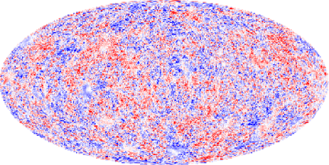
FIG. 1.: CMB for $\Omega_{0}=0.3$ using the Mollweide projection.

FIG. 2.: CMB for $\Omega_{0}=0.6$ using the Mollweide projection.

FIG. 3.: The dependence of $k_{n}^{3/2}f_{n}(\eta)$ on the eigenvalue $E_{n}$ for the case $\Omega_{0}=0.3$ is shown, where $\eta_{0}=2.3746$ and $\alpha=1$. The upper full curve corresponds to $E_{n}=100$ and the lowest one to $E_{n}=3000$. For the intermediate curves the energy is increased in steps of 100. The dashed curve represents the result $f_{\hbox{{mat}}}(\eta)=5(\sinh^{2}\eta-3\eta\sinh\eta+4\cosh\eta-4)/(\cosh\eta-1)^{3}$ belonging to a pure matter model with $c_{s}=0$ used in some related works.

The CMB is computed for different densities $\Omega_{0}$ with respect to the Hubble constant $h=0.6$ in units of $100\hbox{ km }\hbox{s}^{-1}\hbox{Mpc}^{-1}$. The radiation density $\varepsilon_{r}$ is chosen in agreement with the present background radiation temperature of $T=2.728\hbox{ K}$. In figures 1 and 2 the fluctuations of the CMB are shown for $\Omega_{0}=0.3$ and $0.6$, respectively. The monopole and the dipole contribution is subtracted such that the first non-vanishing multipole is the quadrupole in accordance with the usual representation of the CMB fluctuations.

A quantitative measure of the scale of the fluctuations is provided by the angular power spectrum $C_{l}$ defined by

$$C_{l}\;=\;\frac{1}{2l+1}\,\sum_{m=-l}^{l}|a_{lm}|^{2}\hskip 10.0pt,$$

where $a_{lm}$ are the expansion coefficients of $\delta T$ with respect to the spherical harmonics $Y_{l}^{m}(\theta,\phi)$. In the following the angular power spectrum $C_{l}$ is compared with the data measured for $l<30$ by COBE [36], around $l\sim 100$ by QMAP [37] and above $l\sim 80$ by the Saskatoon experiment [38]. These experiments provide evidence that the angular power spectrum increases up to a maximum around $l\simeq 200$.

The figures 1 and 2 show fluctuations on finer scales with decreasing density $\Omega_{0}$. This is due to the cut-off in the wavenumbers $k_{n}<k_{\hbox{{max}}}$. For a genuine Harrison-Zel’dovitch spectrum having no cut-off there are fluctuations on all scales. However, the amplitudes belonging to the different scales depend on $\Omega_{0}$ by the specific form of decay of $f_{n}(\eta)$ via the ISW. The decay of $f_{n}(\eta)$ is faster for smaller densities $\Omega_{0}$ with increasing eigenvalue $E_{n}$ as shown in figure 3 for $\Omega_{0}=0.3$. An estimate of the angular contributions which are maximally taken into account in the angular power spectrum $C_{l}$ for a given $k_{\hbox{{max}}}$ can be obtained as follows. The smallest wavelength $\lambda_{\hbox{{min}}}\simeq\frac{2\pi}{k_{\hbox{{max}}}}$ of the eigenmodes determines the finest scale of the fluctuations on the SLS. The angle $\Theta_{k}$ under which the smallest scale fluctuations are seen, is given by

$$\tan\frac{\Theta_{k}}{2}\;=\;\frac{\tanh\frac{\lambda_{\hbox{{min}}}}{2}}{\sinh(\eta_{0}-\eta_{\hbox{{SLS}}})}\hskip 10.0pt.$$

Since the $l$th spherical harmonics has along the “circumference” $2l$ zeros in $[-180^{\circ},180^{\circ}]$ one gets the rule of thumb that a given $\Theta$ corresponds roughly to $l\simeq 180^{\circ}/\Theta$. In table I the distance $\eta_{0}-\eta_{\hbox{{SLS}}}$, the angle $\Theta_{k}$ under which $\lambda_{\hbox{{min}}}$ appears and the corresponding angular contribution $l_{k}:=180^{\circ}/\Theta_{k}$ are given for several values of $\Omega_{0}$.

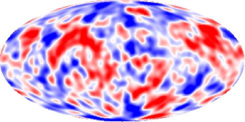
FIG. 4.: A Gaussian smoothing of figure 1, i. e., the case $\Omega_{0}=0.3$, is shown with a resolution of $10^{\circ}$.

To get an impression of the fluctuations as seen with the $10^{\circ}$ resolution of COBE, a Gaussian smoothing of figure 1, i. e., for $\Omega_{0}=0.3$, is presented in figure 4 with that resolution.

The figures 5 to 8 show the angular power spectrum for $\Omega_{0}=0.2,0.3,0.4$ and $0.6$, where the abscissa shows $\sqrt{l(l+1)C_{l}/2\pi}$ in $\mu\hbox{K}$. The data for the compact hyperbolic models are shown up to roughly $l_{k}$. A reasonable agreement is observed for $\Omega_{0}\simeq 0.3\dots 0.4$. In the case $\Omega_{0}=0.2$ $C_{l}$ increases too fast with increasing $l$ in comparison with the experimental data. For $\Omega_{0}=0.4$ one observes a saturation above $l\simeq 40$. Then the further increase of the $C_{l}$ has to come from processes, like acoustic oscillations, getting important on scales of the horizon size at the SLS around $l_{H}=200\dots 300$, see table I. The necessary contributions are not considered here but the results obtained from simply-connected models should then apply since the corresponding scales are small in comparison with the size of the fundamental cell. Further effects like the reionization, gravitational lensing and the Sunyaev-Zel’dovitch effect influence the fluctuations on a scale of order $\Theta\simeq 1^{\circ}$ and thus the values of $C_{l}$ for correspondingly large $l$. More important are the low multipoles since they have ruled out a toroidal structure in the case of a flat universe, at least for periodicities significantly below the horizon size [5, 6, 9]. In the flat case the first multipoles were too small in comparison with the multipoles around $l\simeq 20$. Such an effect is absent in the hyperbolic case and thus a “small” universe is not ruled out. This result is at variance with [23] where agreement with COBE is only obtained for very high densities $\Omega_{0}\simeq 0.8$.

FIG. 5.: The angular power spectrum $\sqrt{l(l+1)C_{l}/2\pi}$ for $\Omega_{0}=0.2$ for the hyperbolic model (full dots) in comparison with the COBE $(\square)$, Saskatoon $(\triangle)$ and QMAP $(\bigcirc)$ data.

FIG. 6.: The angular power spectrum $\sqrt{l(l+1)C_{l}/2\pi}$ for $\Omega_{0}=0.3$ with the same symbols as in figure 5.

FIG. 7.: The angular power spectrum $\sqrt{l(l+1)C_{l}/2\pi}$ for $\Omega_{0}=0.4$ with the same symbols as in figure 5.

FIG. 8.: The angular power spectrum $\sqrt{l(l+1)C_{l}/2\pi}$ for $\Omega_{0}=0.6$ with the same symbols as in figure 5.

In order to show the increasing significance of the ISW with decreasing $\Omega_{0}$, table I shows the rms of the two terms in (9) using $\alpha=1$ in (7). The rms value of the NSW is nearly constant because the fluctuations are determined by (7), i. e., by $\alpha$ independently of the distance to the SLS. In contrast the ISW diminishes towards $\Omega_{0}=1$. For $\Omega_{0}=1$ no ISW contribution occurs because of $d\Phi/d\eta=0$ in this case. The figure 9 shows the contributions to the $C_{l}$ spectrum separately for the NSW and for the ISW as well as both contributions together as observed in nature. The case $\Omega_{0}=0.4$ is shown with $\alpha=1$. The importance of the eigenmodes with respect to the contribution to the ISW is determined by two competing effects. On the one hand higher eigenmodes are oscillating faster such that their contribution to the integral is less important. However, also the derivative $f_{n}^{\prime}(\eta)$ determines the significance, and it is this derivative which increases with increasing eigenvalues as can be inferred from figure 3. Numerically both effects seem to cancel such that the ISW is nearly constant with respect to $C_{l}$. At $\Omega_{0}=0.3$ the NSW and the ISW are of equal significance and for less values of $\Omega_{0}$ the ISW dominates. This can lead to difficulties in detecting paired circles.

FIG. 9.: For $\Omega_{0}=0.4$ the individual contributions of the NSW $(\square)$ and the ISW $(\triangle)$ to the angular power spectrum $\sqrt{l(l+1)C_{l}/2\pi}$ are shown as well as their combined effect (full dots) $(\alpha=1)$.

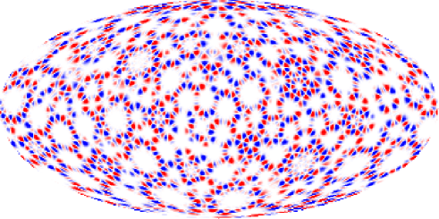
FIG. 10.: The NSW contribution of the lowest eigenmode $(E_{1}\simeq 93.11)$ to the CMB is shown for the case $\Omega_{0}=0.2$.

FIG. 11.: The $C_{l}$ spectrum is shown for the NSW contribution of figure 10. Here $C_{l}$ is shown instead of $\sqrt{l(l+1)C_{l}/2\pi}$ as in the other figures. The scaling at the abscissa is arbitrarily.

It is interesting to note that the large scale power is not only caused by the lowest eigenmodes but also by the large scale structure generated by the isometry group describing the fundamental cell. To stress that fact figure 10 shows the NSW contribution of the lowest eigenmode having an eigenvalue $E_{1}\simeq 93.11$ which has only one maximum within the tetrahedral cell. One clearly observes large circles of different radii having a scale larger than the wavelength of the eigenmode. The $C_{l}$ spectrum, shown in figure 11, has a periodic structure with different maxima corresponding to the circles of different radii and to the structure formed by the arrangement of the circles itself. Only the wide last maximum around $l=60$ corresponds to the peak expected from the wavelength of the lowest eigenmode. If the peaks due to the circles are pronounced enough in comparison with the ISW, there could survive a periodic structure in the full $C_{l}$ spectrum yielding some information about the isometry group.

In conclusion small hyperbolic universes are not ruled out in contrast to the flat case. A reasonable agreement with the experimental data is provided by the hyperbolic models with densities around $\Omega_{0}\simeq 0.3\dots 0.4$. In this work an orbifold instead of a manifold is investigated, however, the statistical properties of the eigenmodes are expected to be the same for orbifolds and manifolds. Thus, since the volume of the considered pentahedron is of the same order as of the Weeks and Thurston manifolds, the comoving wavenumbers $k_{n}$ of these models are comparable since their mean behaviour is determined by Weyl’s law. (Weyl’s law, which counts the mean number of eigenvalues below a given energy, is derived in [29] for general orbifolds.) In these models no supercurvature modes are expected which are absent in the considered pentahedron and could, if present, alter the angular power spectrum. The individual details of the sky maps would differ between the models, but the angular power spectra should show the same behaviour. However, the details of the maps already depend on the locations of the observer within the given fundamental cell. After all, such a small universe has a uniform CMB because in all directions the fluctuations of the same fundamental cell contribute to the CMB and thus circumvents the horizon problem. In addition, the Machian paradox is solved in a new manner by the non-trivial topology. A future work will include the cosmological constant $\Lambda$ in order to investigate its effect on the structure of the CMB.

$\Omega_{0}$	$\Theta_{H}$	$l_{H}$	$\eta_{0}-\eta_{\hbox{{SLS}}}\;$	$\Theta_{k}\;$	$l_{k}\;$	rms of NSW	rms of ISW
0.2	0.46∘	391	2.7527	0.8∘	215	0.066	0.106
0.3	0.60∘	300	2.3214	1.3∘	139	0.066	0.079
0.4	0.73∘	247	1.9863	1.8∘	98	0.067	0.064
0.6	0.94∘	191	1.4409	3.3∘	55	0.070	0.044
0.8	1.12∘	161	0.9322	6.1∘	30	0.069	0.026

TABLE I.: The angle $\Theta_{H}$, under which the horizon at the SLS is seen, the corresponding $l_{H}:=180^{\circ}/\Theta_{H}$, the distance to the SLS, the angle $\Theta_{k}$ due to the cut-off $k_{\hbox{{max}}}$ and the corresponding $l_{k}$ are shown as well as the rms of the NSW and the ISW contribution, respectively, in (9) for $\alpha=1$.