Constraints on a non-Gaussian ($\chi_{m}^{2}$) CDM model

Abstract

We consider constraints on the structure formation model based on non-Gaussian fluctuations generated during inflation, which have $\chi_{m}^{2}$ distributions. Using three data sets, the abundance of the clusters at $z=0$, moderate $z$ and the correlation length, we show that constraints on the non-Gaussianity and the amplitude of fluctuations and the density parameter can be obtained. We obtain an upper bound for $\Omega_{m}$ and a lower bound for the non-Gaussianity and the amplitude of the fluctuations. Using the abundance of clusters at $z\sim 0.6$, for the spectrum parameterized by cold dark matter (CDM) shape parameter $\Gamma=0.23$, we obtain an upper bound for the density parameter $\Omega_{m}\sim 0.5$ and lower bounds for the amplitude $\sigma_{8}\sim 0.7$ and for the non-Gaussianity of fluctuations $G\sim 2$ $(m\sim 200)$, where $G=1$ for Gaussian.

1 Introduction

It is generally accepted that the primeval density fluctuations have grown gravitationally to form the present structure of the Universe. Many models based on Gaussian adiabatic fluctuations generated during inflation have been discussed. However, the standard CDM model, i.e. the structure formation model in a spatially flat universe filled with cold dark matter which has Gaussian adiabatic fluctuations, suffers from several problems. One of the most severe problems is the lack of the cluster abundance at moderate $z$. This is caused by the fact that in a flat universe filled with the matter, fluctuations grow rapidly. To overcome this problem, a low-density universe model, with or without cosmological constant has been investigated extensively.

Recently an alternative was proposed, a model based on non-Gaussian isocurvature fluctuations produced by massive scalar fields frozen during inflation, which have $\chi_{m}^{2}$ distributions (Peebles 1997a,1999a,b). The most notable point of this model is the early formation of objects because of its non-Gaussianity. If the probability distribution function (PDF) has a broad tail compared with a Gaussian PDF, the evolution of clusters becomes slow. In this model there are three important parameters; the amplitude and the non-Gaussianity of the fluctuations and the background density parameter. It is important to explore methods of constraining these parameters.

It is recognized that the non-Gaussianity affects the correlation length of clusters. Robinson, Gawiser $\&$ Silk (1998) suggest that by combining the observations of the abundance of clusters at $z=0$ and the correlation length, constraints on the amplitude and the non-Gaussianity of the fluctuations are obtained simultaneously for a fixed density parameter $\Omega_{m}$. As mentioned above, because the density parameter and the non-gaussanity affect the evolution of abundance, the observations of the abundance of clusters at moderate $z$ give another strong constraint on the model. Much work on the effect of changing $\Omega_{m}$ on the evolution have been carried out assuming Gaussian initial conditions (Frenk et al. 1990; Eke et al. 1996; 1998; Viana $\&$ Liddle 1996,1998; Fan et al. 1997; Bahcall $\&$ Fan 1998; Henry 1997; Carlberg et al 1997). Little work has been carried out, however, on the effect of the non-Gaussianity, except for a topological defect model (Chui $\&$ Ostricker 1998).

In this paper, we extend Press-Schechter (PS) theory to non-Gaussian initial conditions and make clear how the non-Gaussianity affects the evolution of abundance and the bias. Then we show that combining the observations of the abundance of clusters at moderate $z$ with the method proposed by Robinson.et.al, we can obtain a constraint on background cosmology and fluctuations simultaneously: an upper bound for $\Omega_{m}$ and a lower bound for the non-Gaussianity and the amplitude of the fluctuations.

2 Mass function and bias: for Non-Gaussian initial conditions

We extend PS theory (Press $\&$ Schechter 1974; Bond et al. 1991) to non-Gaussian initial conditions and calculate the mass function and the bias of clusters.

In PS theory, the region of the scale $R$ with overdensity greater than a critical amount $\delta_{c}$ is collapsed to form a bound object of mass $M=(4\pi/3)\bar{\rho}R^{3}$, where $\bar{\rho}$ is the mean density of the universe. The threshold is assumed to be given by the spherical collapse model. For Gaussian initial conditions, it has been shown to be a good approximation (Lacey $\&$ Cole 1993). We assume that this approximation is good for non-Gaussian initial conditions. The probability of a region with mass $M$ collapsing at redshift $z_{1}$ is given by

$$F(\delta_{1},M)=\int^{\infty}_{\delta_{1}}P(\delta)d\delta,\quad\delta_{1}=\frac{\delta_{c}}{D(z_{1})},$$ (1)

where $P(\delta)$ is the PDF in question and $D(z)$ is a linear growth factor. According to Jedamzick, the above quantity can be written as

$$F(\delta_{1},M)=\frac{1}{\bar{\rho}}\int^{\infty}_{M}M^{\prime}n(M^{\prime},z_{1})P(M|M^{\prime})dM^{\prime},$$ (2)

where $n(M,z_{1})$ is the mass function at $z=z_{1}$ and $P(M|M^{\prime})$ denotes the probability of finding a region with mass $M$ overdense by $\delta_{1}$ or more, provided it is included in an isolated overdense region with mass $M^{\prime}$ (Jedamzick 1995). We assume this quantity is given by

$$P(M|M^{\prime})=P(\delta_{M}\geq\delta_{1}|\delta_{M^{\prime}}=\delta_{1})=\int^{\infty}_{\delta_{1}}P(\delta|\delta_{1})d\delta\equiv 1/f,$$ (3)

where $P(\delta|\delta_{1})$ is a conditional probability function. Hence, the mass function $n(M,z_{1})$ is given by

$$n(M,z_{1})=-\frac{f\bar{\rho}}{M}\frac{dF(\delta_{1},M)}{dM}.$$ (4)

The bias of the bound objects can be calculated using the formalism developed by Mo and White (Mo $\&$ White 1996). Consider the collapsed region of scale $R_{1}$ with over-density $\delta_{1}$ and the uncollapsed region of $R_{0}$ with $\delta_{0}$. If at present $\delta_{1}$ = $\delta_{c}/D(z_{1})$, then the halo is identified as being formed at $z_{1}$. The number of objects of $M_{1}$ identified at $z_{1}$ in a spherical region with a comoving radius $R_{0}$ is

$$N(1|0)dM_{1}=-f\frac{M_{0}}{M_{1}}\frac{d}{dM_{1}}\int^{\infty}_{\delta_{1}}d\delta P(\delta|\delta_{0}).$$ (5)

Thus, the average overdensity of objects in the sphere of radius $R_{0}$ relative to the global mean halo abundance becomes

$$\delta^{L}_{cl}(1|0)=\frac{N(1|0)}{n(M,z)V_{0}}-1$$ (6)

in Lagrangian space (Mo $\&$ White 1996).

If the region $0$ is sufficiently large compared with region $1$ ( $R_{0}\gg R_{1}$, $\langle\delta_{1}^{n}\rangle\gg\langle\delta_{0}^{n}\rangle$), regardless of the statistics, the relation

$$\langle\delta_{1}^{p}\delta_{0}^{n-p}\rangle=\langle\delta_{0}^{n}\rangle$$ (7)

is satisfied (Appendix A) and the conditional probability is given by

$$P(\delta_{1}|\delta_{0})=P(\delta_{1}-\delta_{0}).$$ (8)

(Appendix B). If this is the case, we obtain the normalization of the mass function

$$f=1/(\int^{\infty}_{0}P(\delta)d\delta),$$ (9)

which agrees with the one introduced to ensure that all the mass in the universe is accounted for (Lucchin and Matarrese 1989, Chui and Ostriker 1998). Since

$$N(1|0)dM=-f\frac{M_{0}}{M_{1}}\frac{d}{dM_{1}}\int^{\infty}_{\delta_{1}-\delta_{0}}d\delta P(\delta),$$ (10)

the overdensity of the bound objects is given by

$$\delta^{L}_{cl}=\frac{n(1|0)-n(M)}{n(M)},\quad\quad n(1|0)=n(M)|_{\delta_{1}\to\delta_{1}-\delta_{0}}.$$ (11)

This reproduces the peak-background split formalism (Kaiser 1984; Bardeen et al. 1986; Robinson et al. 1998).

Furthermore, we assume that reduced moments

$$\lambda_{N}=\frac{\langle\delta^{N}\rangle}{\langle\delta^{2}\rangle^{N/2}}$$ (12)

do not depend on mass $M$ on the relevant scales.

In the following discussion, we make these assumptions and use above formalisms. Note that the accuracy required to use Press-Schechter theory for non-Gaussian initial conditions is currently uncertain. One way to confirm its validity is to perform N-body simulations. Recently Baker and Robinson have carried out N-body simulations for several non-Gaussian models to show mass function of PS formalism agrees well with that observed in simulations (Robinson & Baker1999). It will be necessary to perform further detailed tests of the accuracy of this formalisms, especially for the bias model.

3 The abundance and the bias of the bound objects.

We use the formalisms developed in the previous section and investigate the effect of non-Gaussianity on the evolution of abundance and the bias of the bound objects. First we consider the evolution of the number density. We define the rate of change with $z$ of the number density by

$$\triangle n(M,z)=-\frac{1}{n(M,z)}\frac{dn(M,z)}{dz}.$$ (13)

This can be written as

$$\triangle n(M,z)=\left[-\frac{d\log\nu P(\nu)}{d\nu}\right]_{\nu(M,z)}\left(-\frac{d\log D(z)}{dz}\right)\nu(M,z),$$ (14)

where

$$\nu(M,z)=\frac{\delta_{c}}{\sigma(M)D(z)},\quad\sigma(M)=\sigma_{8}\left(\frac{M}{M_{\ast}}\right)^{-(3+n)/6},$$ (15)

where $M_{\ast}$ is the mass contained in the spherical region of $8h^{-1}$ Mpc and $n$ is the spectrum index. This indicates that for a fixed PDF, if fluctuations decrease slow with $z$ (as in low $\Omega_{m}$ universe), the number density also decreases slowly with $z$. We fix the background cosmology and compare the evolution of the number density for different PDFs. The difference of this quantity between a Gaussian PDF and the PDF in question can be written as

$$\triangle n_{G}-\triangle n=\left[\frac{d\log g(\nu)}{d\nu}\right]_{\nu(M)}\left(-\frac{d\log D(z)}{dz}\right)\nu(M).$$ (16)

Here $g(\nu)$ denotes the ratio of the PDF to a Gaussian PDF:

$$g(\nu)=\frac{P(\nu)}{P_{G}(\nu)},$$ (17)

where $P_{G}$ is a Gaussian PDF. Next we calculate the bias of clusters at the present time. The linear bias $\delta_{cl}=b\delta$ in Eulerian space is given by

$$b(M)=1-\frac{d\log n(M)}{d\delta_{c}}.$$ (18)

The difference from a Gaussinan PDF is given by

$$b_{G}(M)-b(M)=\left[\frac{d\log g(\nu)}{d\nu}\right]_{\nu(M)}\frac{1}{\sigma(M)},$$ (19)

where the bias for a Gaussian PDF is

$$b_{G}(M)=1+\frac{\nu(M)^{2}-1}{\delta_{c}}$$ (20)

(Cole $\&$ Kaiser 1989; Mo $\&$ White 1996).

If a PDF has a broad tail compared with a Gaussian PDF, therefore, the number density of the objects $M$ evolves slowly with $z$ and the bias of such objects is small compared with those for a Gussian PDF. This is natural because these rare objects can be formed easily for a PDF with a broad tail.

4 The $\chi^{2}$ model

In this section, we investigate the $\chi_{m}^{2}$ model ( Coles and Barrow 1987, Moscardini et.al 1991, Weinberg and Coles 1992). In this model, fluctuations are drawn from $\chi_{m}^{2}$ distributions. Peebles gives one realization of this model in the framework of inflationary universe(Peebles 1997,1999a). In his model, CDM fields are squeezed massive scalar fields which have $O(N)$ symmetry. The isocurvature perturbations are generated during inflation. The density and the over-density of CDM fields are given by

$$\rho_{CDM}=\frac{\mu}{2}\sum^{m}_{i=1}\phi_{i}^{2},\quad\delta=\frac{1}{m\langle\phi^{2}\rangle}\sum^{m}_{i=1}\phi_{i}^{2}-1,$$ (21)

where $m$ is the number of the CDM fields $\phi$, which have $O(m)$ symmetry and a Gaussian PDF and $\mu$ is the mass of the CDM fields. Then, the PDF of the overdensity is given by

$$P(\nu)d\nu=\frac{(1+\sqrt{\frac{2}{m}}\nu)^{m/2-1}}{(\frac{2}{m})^{(m-1)/2}\Gamma(\frac{m}{2})}\exp\left(-\frac{m}{2}\left(1+\sqrt{\frac{2}{m}}\nu\right)\right)d\nu.$$ (22)

If the autocorrelation function of the Gaussian field $\phi(\mbox{\boldmath$x$})$ is $\xi_{\phi}=\langle\phi(\mbox{\boldmath$x$}_{1})\phi(\mbox{\boldmath$x$}_{2})\rangle\propto x_{12}^{-\epsilon}(x_{12}=|\mbox{\boldmath$x$}_{1}-\mbox{\boldmath$x$}_{2}|$), the autocorrelation function and the reduced moments of $\delta$ are given by

$$\xi(x_{12}) = \langle\delta(\mbox{\boldmath$x$}_{1})\delta(\mbox{\boldmath$x$}_{2})\rangle=\left(\frac{2}{m}\right)\frac{\xi_{\phi}^{2}(x_{12})}{\langle\phi^{2}\rangle}$$

$$\lambda_{N} = (N-1)!\left(\frac{2}{m}\right)^{N/2-1}\frac{(\langle x_{12}x_{23}\cdot\cdot x_{N-1N}x_{N1})^{-\epsilon}\rangle}{\langle x_{12}^{-2\epsilon}\rangle^{(N/2)}},$$

where angular brackets denote averaging on some smoothing length (Peebles 1999b).

Note that two problems seem to exist in this model. First, because the autocorrelation function is positive for all separations, the integral of $\xi(r)$ over all space does not vanish (White 1998). Next it can be shown that the reduced moments remain approximately same for a variety of smoothing scales if $\epsilon$ is scale-invariant(Peebles 1999b, White 1998). This seems to be in contradiction to the central limit theorem that states all distributions must become Gaussian when smoothed on sufficiently large scales. If desired, however, it is possible to modify the Peebles model so that these difficulties disappear. For example, an off-centered $\chi^{2}_{m}$ model, where $\rho=\mu/2\sum(\phi_{i}-\phi_{0})^{2}$, produces a distribution that is non-Gaussian on small scales and Gaussian on large scales. This scale is determined by the mass scale $\phi_{0}$. Here, we are interested in the scale relevant to cluster formation where $\xi$ has a power-low spectrum for which $\xi>0$ and the smoothing length is not so large, so we believe that these technical difficulties do not affect us. Indeed, our method can be applied to any non-Gaussian model on this scale.

In the $\chi_{m}^{2}$ model the non-Gaussianiy is represented by one parameter $m$. As the effect of the non-Gaussianity depends on the broadness of the PDF, we introduce another parameter $G$ to represent the amount of deviation from Gaussianity:

$$G=\sqrt{2\pi}\int_{3}^{\infty}P(\nu)d\nu/\int_{3}^{\infty}e^{-\nu^{2}/2}d\nu,$$ (24)

which is the likelyhood relative to Gaussian of $3\sigma$ or rare events (Robinson et al. 1998). $G$ is related to $m$ as follows:

$m$	1	8	32	200	$\infty$
$G$	16.3	7.66	4.02	2.04	1

5 Evolution of abundance and correlation length of clusters

We examine the evolution of the number density of rich clusters from $z=0$ to $z=1$. We consider the clusters with the mass $M(<R_{com}=1.5h^{-1}\mbox{Mpc})>8\times 10^{14}M_{\odot}$, where $M(<R_{com})$ represents the mass contained within the comoving length $R_{com}$ (Bahcall $\&$ Fan 1998). The number density of such clusters is given by

$$N(M(<R_{com}=1.5h^{-1}\mbox{Mpc})>8\times 10^{14}M_{\odot})=\int^{\infty}_{M_{lim}}n(M)dM.$$

We relate the mass threshold $M(<R_{com}=1.5h^{-1}\mbox{Mpc})=8\times 10^{14}M_{\odot}$ to the virial mass $M_{lim}$ using the density profile $M(<R)\propto R^{0.64}$ (Bahcall $\&$ Fan 1998). The result is shown for different $\Omega_{m}$ ($G=1$, $\Lambda=1-\Omega_{m}$) and $G$ ($\Omega_{m}=1$) in Fig.1. The Gaussian model in the universe of $\Omega_{m}=1$ is strongly disfavored (Calberg et al 1997; Bahcall $\&$ Fan 1998). The non-Gaussianity of fluctuations makes the evolution of the abundance slow.

Figure 1: The evolution of cluster abundance of $M(<R_{com}=1.5h^{-1}Mpc)>8\times 10^{14}M_{\odot}$ clusters for a different $\Omega_{m}$ ($G=1$, $\Lambda=1-\Omega_{m}$, upper panel) and for a different $G$ ($\Omega_{m}=1$, lower panel).

The correlation length $r_{0}$ of clusters with the mean separation $d=N(>R)^{-1/3}$ is obtained as follows (Robinson et al. 1998). Using the mass function we obtain the scale $R$ of clusters with the mean separation $d=N(>R)^{-1/3}$. Then, the amplitude of two-point correlation function of matter fluctuations at correlation length is given by $\xi_{m}=1/b(R)^{2}$. If we know $\sigma_{8}$ and the spectrum index, $n$, we can obtain the correlation length. The bias is given by

$$b=1+\frac{\nu^{2}-1}{\delta_{c}(1+\sqrt{\frac{2}{m}}\nu)}.$$ (25)

For large $G$ (small $m$), the bias becomes small and the correlation length becomes short. We fix $\sigma_{8}=0.5$, $n=-1.4$ and $\Omega_{m}=1$; the bias and correlation length of the clusters with mean separation $d=30h^{-1}$ Mpc are then given as follows:

$G$	16.3	7.66	4.02	2.04	1
$b_{1}$	1.8	2.4	2.7	3.1	3.4
$r_{0}$	6.9	10.0	11.9	13.6	15.3

6 Constraints on $\Omega_{m}$, $G$ and $\sigma_{8}$

We can give constraints on $\Omega_{m}$, $G$ and $\sigma_{8}$ by using the abundance of the rich clusters at $z=0$, $z=0.575$ and the correlation length. We use the following data sets.

• The abundance of $M(<R_{com}=1.5)>8\times 10^{14}h^{-1}M_{\odot}$ clusters at z=0 is taken from temperature function of $T>6.4$ kev (Bahcall $\&$ Fan 1998). We use $2^{+2}_{-1}\times 10^{-7}h^{3}$Mpc^-3 (Henry $\&$ Arnaud 1991).

• The abundance at z=0.575 is taken from the data of the Einstein Medium Sensitivity Survey (EMSS). We use $n(z=0.5-0.65)=3^{+2.4}_{-1.9}\times 10^{-8}h^{3}$ Mpc^-3 for $\Omega_{m}=1$. The error bars represent $2\sigma$ statistical errors (Bahcall $\&$ Fan 1998). (For $\Omega_{m}<1$ we use $n(z=0.5-0.65)=2^{+2}_{-1}\times 10^{-8}h^{3}$ Mpc^-3.)

• The correlation length is taken from the Automatic Plate Measuring (APM) Survey. We use $r_{0}=14.2^{+0.8}_{-1.0}h^{-1}$Mpc for the clusters of mean separation $d=30h^{-1}$Mpc. The error bars represent $2\sigma$ statistical errors (Croft et al. 1997).

Henceforth, for simplicity, we only investigate the model with a cosmological constant and use the spectrum parameterized by CDM shape parameter $\Gamma$ (Bardeen et al. 1986). We will assume $\Gamma=0.23$ (Vianna $\&$ Liddle 1998).

From the above data sets, we can give constraints on $\Omega_{m}$, $G$ and $\sigma_{8}$ (Fig.2). First, consider the abundance at $z=0$. For large $G$, the clusters are formed easily so we need small $\sigma_{8}$. Since $\sigma_{8eff}=\sigma_{8}\Omega_{m}^{(n+3)/6}$ determines the abundance of clusters, we need large $\sigma_{8}$ for small $\Omega_{m}$. The fit contour runs from the upper left (large $G$ and small $\sigma_{8}$) to the lower right(small $G$ and large $\sigma_{8}$) in the $\sigma_{8}$ vs $G$ plane and this moves to right as $\Omega_{m}$ becomes small. Next, consider the abundance at $z\sim 0.6$. For $\Omega_{m}\sim 1$, if fluctuations are Gaussian ($G=1$), the abundance at $z\sim 0.6$ is too small compared with the data of the EMSS. For large $G$, because of the effect of the non-Gaussianity, the abundance becomes consistent with the observation (Fig.1). The fit contour runs in the plane in the same direction as of $z=0$, but the slope is smaller. As $\Omega_{m}$ decreases, the abundance at $z\sim 0.6$ can be explained even if fluctuations are Gaussian. Then, as $\Omega_{m}$ decreases, the fit contour moves to right more slowly than that of $z=0$. The region that can support these two data sets at the same time therefore exists in the upper left of the plane for large $\Omega_{m}$ and stretches to the lower right as $\Omega_{m}$ becomes small.

Next consider the correlation length. At the scale of the correlation length, the variance of matter fluctuations is given by $\sigma=1/b$. For large $G$, therefore, because the bias $b$ is small, we need large $\sigma_{8}$. The fit contour runs from the lower left to the upper right of the plane, i.e. orthogonal to the fit contours of the abundance (Robinson et al. 1998). The correlation length is mainly determined by the statistics of fluctuations, which does not change as $\Omega_{m}$ changes. The region that supports the correlation length and abundance at $z=0$ therefore moves from lower left to upper right as $\Omega_{m}$ decreases. Now, we combine all the data. For $\Omega_{m}\sim 1$ we cannot find a region that will support all the data sets. As $\Omega_{m}$ decreases, we come to some $\Omega_{m}$, for which the region that supports all the data sets exists. This region moves to the upper right as $\Omega_{m}$ becomes small;  we can then obtain the upper bound for $\Omega_{m}$ and the lower bound for $\sigma_{8}$ and $G$.

From the above data sets, the upper bound $\Omega_{m}<0.5$ and the lower bound $G>2$ and $\sigma_{8}>0.7$ are obtained. Particularly in the universe of $\Omega_{m}=0.3$, which is favored by other observations, non-Gaussianity of the order $G\sim 4$ is favored.

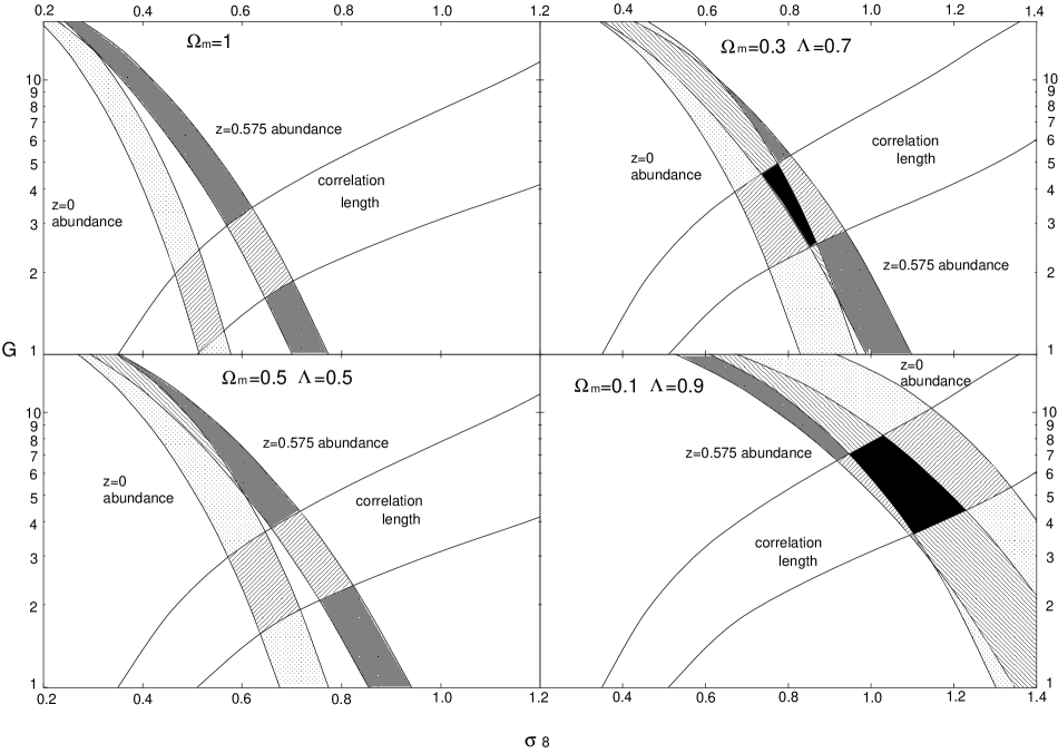
Figure 2: Fit contours of the three data sets in $\sigma_{8}$ vs $G$ plane.

Figure 3: The cumulative cluster temperature function for the $\chi^{2}_{m}$ model at the present time.

The shape of the cluster temperature function could possibly give another constraint on the model (Kitayama and Suto 1996). We show the temperature function at the present time for the parameters that are consistent with all three data sets ($\Omega_{m}=0.3,\Lambda=0.7,G=4.02,\sigma_{8}=0.75$ and $\Omega_{m}=0.1,\Lambda=0.9,G=6.33,\sigma_{8}=1.1$ (Fig.3)). Here we convert the virial mass $M_{v}$ to X-ray temperature using

$$kT=\frac{7.75}{\beta}\left(\frac{M_{v}}{10^{15}h^{-1}M_{\odot}}\right)^{2/3}(1+z)\left(\frac{\Omega_{m}}{\Omega(z)}\right)^{1/3}\left(\frac{\triangle_{v}}{178}\right)^{1/3}\mbox{kev},$$

where $\triangle_{v}$ is the virial over-density ($\triangle_{v}=\rho_{virial}/\rho_{c}$) and we take $\beta=1$ (Eke et al. 1996; 1998; Borgani et al 1998). The shape of the temperature function agrees well with the data of Henry and Arnaud for high temperatures (Henry & Arnaud 1991, Henry 1997). Note that as $\Omega_{m}$ decreases, the non-Gaussianity and $\sigma_{8}$ becomes large, so the slope of the temperature function becomes smaller. Then, the difference in the abundance for different $\Omega_{m}$ is larger for low temperatures. This provides us with the possibility of obtaining another constraint on the low-density universe model.

7 Conclusion

We have given constraints on the $\chi_{m}^{2}$ model, where fluctuations are drawn from $\chi_{m}^{2}$ distributions. We extended the Press-Scheter theory to calculate the abundance and bias of clusters. The non-Gaussianity of fluctuations makes the evolution of the abundance slow. The model with non-Gaussian fluctuations of the order $G\sim 16$ $(m=1)$ in $\Omega_{m}=1$ universe has roughly the same evolution of the number density as a Gaussian model in a $\Omega_{m}=0.2$ universe, where $G$ represents the non-Gaussianity of the fluctuations ($G=1$ for Gaussian). On the other hand, the strong non-Gaussianity of fluctuations make the correlation length too short. Combining the three data sets, the abundance of the clusters at $z=0$ and $z\sim 0.6$ and the correlation length, constraints on the non-Gaussianity and the amplitude of fluctuations and the density parameter have been obtained. We have shown that the upper bound for $\Omega_{m}$ and the lower bound for the non-Gaussianity and the amplitude of the fluctuations can be given. For the spectrum parameterized by CDM shape parameter $\Gamma=0.23$, we have obtained an upper bound for the density parameter $\Omega_{m}\sim 0.5$ and lower bounds for the amplitude $\sigma_{8}\sim 0.7$ and the non-Gaussianity $G\sim 2$ $(m\sim 200)$ of fluctuations. In the universe with $\Omega_{m}=0.3$ and $\Lambda=0.7$, non-Gaussianity of the order $G\sim 4$ $(m\sim 30)$ is preferred.

8 acknowledgment

The authors are grateful to J.Robinson for useful comments. The work of J.S. was supported by Monbusho Grant-in-Aid No.10740118 and the work of K.K. was supported by JSPS Research Fellowships for Young Scientist No.04687.

Appendix A Cross-correlation between scales

In this appendix, we show that if $R_{0}\gg R_{1}$, the relation

$$\langle\delta_{1}^{p}\delta_{0}^{n-p}\rangle=\langle\delta_{0}^{n}\rangle.$$ (26)

is satisfied. This is the extension of the relation for Gaussian initial conditions which was derived by Bower under the assumption that the volume of the region $0$ is sufficiently larger than that of the region $1$ (Bower 1991). The smoothed overdensity in the region of scale $R$ is

$$\delta(\mbox{\boldmath$x$},R)=\int\frac{d^{3}\mbox{\boldmath$k$}}{(2\pi)^{3}}\delta_{\mbox{\boldmath$k$}}W_{R}(kR)e^{-i\mbox{\boldmath$k$}\cdot\mbox{\boldmath$x$}},$$ (27)

where $W_{R}(kR)$ is a smoothing function. The n-point functions of the random field $\delta_{\mbox{\boldmath$k$}}$ are expressed as

$$\langle\delta_{\mbox{\boldmath$k$}_{1}}\delta_{\mbox{\boldmath$k$}_{2}}\rangle = \xi_{2}(\mbox{\boldmath$k$}_{1},\mbox{\boldmath$k$}_{2}),$$

$$\langle\delta_{\mbox{\boldmath$k$}_{1}}\delta_{\mbox{\boldmath$k$}_{2}}\delta_{\mbox{\boldmath$k$}_{3}}\rangle = \xi_{3}(\mbox{\boldmath$k$}_{1},\mbox{\boldmath$k$}_{2},\mbox{\boldmath$k$}_{3})$$

$$\langle\delta_{\mbox{\boldmath$k$}_{1}}\delta_{\mbox{\boldmath$k$}_{2}}\delta_{\mbox{\boldmath$k$}_{3}}\delta_{\mbox{\boldmath$k$}_{4}}\rangle = \xi_{4}(\mbox{\boldmath$k$}_{1},\mbox{\boldmath$k$}_{2},\mbox{\boldmath$k$}_{3},\mbox{\boldmath$k$}_{4})+\xi_{2}(\mbox{\boldmath$k$}_{1},\mbox{\boldmath$k$}_{2})\xi_{2}(\mbox{\boldmath$k$}_{3},\mbox{\boldmath$k$}_{4})$$ (28)

$$+cycl.\>(\mbox{2-terms}).$$

Consider the region $1$ with scale $R_{1}$ centered $\mbox{\boldmath$x$}_{1}$ contained in the region $0$ with scale $R_{0}$ centered $\mbox{\boldmath$x$}_{0}$. The variance of the overdensity in the region $i$ is

$$\sigma^{2}(R_{i})=\langle\delta_{i}^{2}\rangle=\int\frac{d^{3}\mbox{\boldmath$k$}}{(2\pi)^{3}}W_{R}^{2}(kR_{i})P(k),$$ (29)

where $P(k)$ is defined by $\xi(\mbox{\boldmath$k$}_{i},\mbox{\boldmath$k$}_{j})=\delta_{D}(\mbox{\boldmath$k$}_{i}+\mbox{\boldmath$k$}_{j})P(k_{i})$. The covariance is written as

$$\sigma^{2}(R_{0}R_{1})=\langle\delta(R_{0})\delta(R_{1})\rangle$$ (30)

$$=\int\frac{d^{3}\mbox{\boldmath$k$}}{(2\pi)^{3}}P(k)W(kR_{0})W(kR_{1})\langle e^{-i\>\mbox{\boldmath$k$}\cdot\mbox{\boldmath$y$}}\rangle_{1\in 0},$$

where $\mbox{\boldmath$y$}=\mbox{\boldmath$x$}_{0}-\mbox{\boldmath$x$}_{1}$. Averaging over $y$ is done as follows: select a random set of points $y$ for which all points in the region $1$ are independent and enclosed in the region $0$, then average over this random set of $y$. The averaged term can be written to appear like another window function

$$\tilde{W}_{\tilde{R}}(k\tilde{R}) = \langle e^{-i\mbox{\boldmath$k$}\cdot\mbox{\boldmath$y$}}\rangle_{1\in 0}$$ (31)

$$= \int_{\tilde{R}}d^{3}\mbox{\boldmath$y$}\>w(\mbox{\boldmath$y$})e^{-i\mbox{\boldmath$k$}\cdot\mbox{\boldmath$y$}}/\int_{\tilde{R}}d^{3}\>\mbox{\boldmath$y$}w(\mbox{\boldmath$y$}),$$

where $\tilde{R}$ is the scale covered by the points $y$ for which region $1$ lies in region $0$. The weight function $w(\mbox{\boldmath$y$})$ is defined so that every point in the region $0$ has an equal chance of contributing to the average density measured in the region 1. Then we can write the real-space window function of the region $0$ as the convolution

$$W_{R_{0}}(\mbox{\boldmath$x$})=\int d^{3}\mbox{\boldmath$x$}^{\prime}W_{R_{1}}(\mbox{\boldmath$x$})\tilde{W}_{\tilde{R}}(\mbox{\boldmath$x$}-\mbox{\boldmath$x$}^{\prime}).$$ (32)

In Fourier space

$$W_{R_{0}}(kR_{0})=\tilde{W}_{\tilde{R}}(k\tilde{R})W_{R_{1}}(kR_{1}).$$ (33)

Note that it is possible to find real weighting function only if the region $1$ is sufficiently small compared to the region $0$, i.e. $R_{0}\gg R_{1}$. If this is the case, the covariance is given by

$$\sigma^{2}(R_{0}R_{1})=\int\frac{d^{3}\mbox{\boldmath$k$}}{(2\pi)^{3}}W_{R}^{2}(kR_{i})P(k)=\sigma^{2}(R_{0}).$$ (34)

Extensions to the higher moments are quite similar. For example,

$$\langle\delta_{1}^{p}\delta_{0}^{n-p}\rangle$$ (35)

$$= \int d^{3}\mbox{\boldmath$k$}_{1}\cdot\cdot d^{3}\mbox{\boldmath$k$}_{n}\delta_{D}^{3}(\mbox{\boldmath$k$}_{1}+\cdot\cdot\mbox{\boldmath$k$}_{n})\langle\delta_{\mbox{\boldmath$k$}_{1}}\cdot\cdot\cdot\delta_{\mbox{\boldmath$k$}_{n}}\rangle$$

$$\times W_{R_{0}}(k_{1}R_{0})\cdot\cdot\cdot W_{R_{0}}(k_{n-p}R_{0})$$

$$\times[W_{R_{1}}(k_{n-p+1}R_{1})\tilde{W}_{\tilde{R}}(k_{n-p+1}\tilde{R})]\cdot\cdot\cdot$$

$$\times[W_{R_{1}}(k_{n}R_{1})\tilde{W}_{\tilde{R}}(k_{n}\tilde{R})]$$

$$= \int d^{3}\mbox{\boldmath$k$}_{1}\cdot\cdot d^{3}\mbox{\boldmath$k$}_{n}\delta_{D}^{3}(\mbox{\boldmath$k$}_{1}+\cdot\cdot\mbox{\boldmath$k$}_{n})\langle\delta_{\mbox{\boldmath$k$}_{1}}\cdot\cdot\cdot\delta_{\mbox{\boldmath$k$}_{n}}\rangle$$

$$\times W_{R_{0}}(k_{1}R_{0})\cdot\cdot\cdot W_{R_{0}}(k_{n}R_{0})$$

$$= \langle\delta_{0}^{n}\rangle.$$

Appendix B Conditional probability

We will derive the Edgeworth expansion (Bernardeau $\&$ Kofman 1995; Juszkiewicz et al. 1995) for the conditional probability of $\delta_{0}$ and $\delta_{1}$ in the case that $R_{0}\gg R_{1}$ is satisfied. The generating function for joint moments

$$C(\mu,\nu)=\int d\delta d\theta e^{i\mu\delta+i\nu\theta}P(\delta,\theta)$$ (36)

gives rise to

$$\langle\delta^{n}\theta^{m}\rangle=\left.\frac{\partial^{n+m}C(\mu,\nu)}{\partial(i\mu)^{n}\partial(i\nu)^{m}}\right|_{\mu=\nu=0}.$$ (37)

The characteristic function becomes

$$K(\mu,\nu)=\log C(\mu,\nu)=\sum^{\infty}_{(n,m)\neq(0,0)}\frac{(i\mu)^{n}(i\nu)^{m}}{n!m!}\lambda_{nm},$$ (38)

where connected joint moments

$$\lambda_{mn}=\langle\delta^{n}\theta^{m}\rangle_{c}$$ (39)

are used. The inverse transformation gives the conditional probability function

$$P(\delta,\theta)=\frac{1}{(2\pi)^{2}}\int d\mu d\nu e^{-i\mu\delta-i\nu\theta}e^{K(\mu,\nu)}$$ (40)

$$=\frac{1}{(2\pi)^{2}}\int d\mu d\nu e^{-i\mu\delta-i\nu\theta-\frac{1}{2}\mu^{2}-\frac{1}{2}\nu^{2}-r\mu\nu}e^{\Sigma(\mu,\nu)},$$

where

$$\Sigma(\mu,\nu)=\sum^{\infty}_{N=3}\sum_{m+n=N}\frac{(i\mu)^{n}(i\nu)^{m}}{n!m!}\lambda_{nm}$$ (41)

is the nonlinear part of the characteristic function and $r=\langle\delta\theta\rangle$ is a cross-correlation. Here we rescale $\delta$ and $\theta$ so as to have a unit variance. Simple calculation yields

$$P(\delta,\theta)=e^{\Sigma(i\frac{\partial}{\partial\delta},i\frac{\partial}{\partial\theta})}\>\frac{1}{2\pi\sqrt{1-r^{2}}}\>e^{-\frac{1}{2}\frac{(\delta-r\theta)^{2}}{1-r^{2}}-\frac{1}{2}\theta^{2}}.$$ (42)

To proceed further, we use the relation derived in appendix A:

$$\langle\delta^{N}\rangle=\lambda_{N0},\langle\delta^{p}\theta^{N-p}\rangle=r^{p}\lambda_{0N},\langle\theta^{N}\rangle=\lambda_{0N}.$$ (43)

Now, let us define

$$\alpha=\frac{\delta-r\theta}{\sqrt{1-r^{2}}},\quad\beta=\theta.$$ (44)

We then obtain

$$P(\delta,\theta) = \exp\left(\sum^{\infty}_{N=3}\left[\frac{1}{N!}(\lambda_{N0}-\lambda_{0N}r^{N})\left(-\frac{1}{\sqrt{1-r^{2}}}\frac{\partial}{\partial\alpha}\right)^{N}\right]\right)$$ (45)

$$\times\frac{1}{\sqrt{2\pi}}e^{-\frac{1}{2}\alpha^{2}}P(\theta),$$

where

$$P(\theta)=\exp{\left(\sum^{\infty}_{N=3}\left[\frac{\lambda_{0N}}{N!}\left(-\frac{1}{\partial\beta}\right)^{N}\right]\right)\frac{1}{\sqrt{2\pi}}}e^{-\frac{1}{2}\beta^{2}}$$

$$=\frac{1}{\sqrt{2\pi}}e^{-\frac{\theta^{2}}{2}}\left(1+\frac{\lambda_{3}}{3!}H_{3}(\theta)+O(\lambda_{3}^{2},\lambda_{4})\right).$$ (46)

Here we use the definition of the Hermite functions

$$H_{n}(x)=e^{\frac{x^{2}}{2}}\left(-\frac{d}{dx}\right)^{n}e^{-\frac{x^{2}}{2}}.$$ (47)

Then the conditional probability function is given by

$$P(\delta|\theta)=\frac{P(\delta,\theta)}{P(\theta)}$$ (48)

$$=\exp\left(\sum^{\infty}_{N=3}\left[\frac{1}{N!}(\lambda_{N0}-\lambda_{0N}r^{N})\left(-\frac{1}{\sqrt{1-r^{2}}}\frac{\partial}{\partial\alpha}\right)^{N}\right]\right)$$

$$\times\frac{1}{\sqrt{2\pi}}e^{-\frac{1}{2}\alpha^{2}}.$$

Consider the small region $1$ contained in a large region $0$. Defining the variance $\sigma_{1}$ for $\delta_{1}$ and $\sigma_{0}$ for $\delta_{0}$ and rescaling yields the Edgeworth formula for conditional probability

$$P(\delta_{1}|\delta_{0})=\frac{1}{\sqrt{2\pi}\sqrt{\sigma_{1}^{2}-\sigma_{0}^{2}}}\exp\left[-\frac{(\delta_{1}-\delta_{0})^{2}}{2(\sigma_{1}^{2}-\sigma_{0}^{2})}\right]$$

$$\times\left(1+\frac{\langle\delta_{1}^{3}\rangle-\langle\delta_{0}^{3}\rangle}{3!(\sigma_{1}^{2}-\sigma_{0}^{2})^{3/2}}H_{3}\left(\frac{\delta_{1}-\delta_{0}}{\sqrt{\sigma_{1}^{2}-\sigma_{0}^{2}}}\right)+\cdot\cdot\cdot\right).$$ (49)

Using the relation

$$\langle\delta_{1}^{n}\rangle\gg\langle\delta_{0}^{n}\rangle,$$ (50)

the conditional probability is reduced to

$$P(\delta_{1}|\delta_{0})=P(\delta_{1}-\delta_{0}).$$ (51)

References

• [1] Bahcall,N.A.& Fan,X.,1998. ApJ,504, 1.
• [2] Bardeen,J.M.,Bond,J.R.,Kaiser,N.,& Szalay,A.S.,1986. ApJ,304, 15.
• [3] Bond,J.R.,Cole,S.,Efstathiou,G.& Kaiser,N., 1991. ApJ,379, 440.
• [4] Borgani,S.,Rosati,P.,Tozzi,P. $\&$ Norman,C.,astro-ph/9901017
• [5] Bower,R.G., 1991. MNRAS,248, 332.
• [6] Carlberg, R.G., Morris, S.L., Yee, H.K.C., $\&$ Ellingson, E., 1997, ApJ.479, L19.
• [7] Chui,W.A.& Ostriker,J.P., 1998. ApJ.494, 479.
• [8] Cole,S.& Kaiser,N., 1989. MNRAS,237, 1127.
• [9] Coles,P.& Barrow,J.D.,1987. MNRAS,228, 407.
• [10] Croft,R.A.C.,Dalton,G.B.,Efstathiou,G.,Sutherland,W.J.& Maddox,S.J. astro-ph/9701040.
• [11] Eke,V.R.,Coles,S.& Frenk,C.S., 1996. MNRAS,282, 263.
• [12] Eke,V.R.,Coles,S., Frenk,C.S.& Henry,J.P. astro-ph/9802350.
• [13] Fan,X.,Bahcall,N.A., $\&$ Cen.,R.,1997, ApJ,490, L123.
• [14] Frenk,C.C.,White,S.D.M.,Efstathiou,G. $\&$ David,M.,1990.
ApJ,351, 10.
• [15] Henry,J.P.,1997 ApJ ,489, L1.
• [16] Henry,J.P.& Arnaud,K., 1991. ApJ, 372, 410.
• [17] Jedamzik,K.,1995. ApJ,448, 1.
• [18] Kaiser,N.,1984. ApJ,284, L9.
• [19] Kitayama,T. & Suto,Y.,1996 ApJ, 469, 480.
• [20] Lacey,C.& Cole,S., 1993, MNRAS,262, 627.
• [21] Lucchin,F. & Matarrese,S.,1989 ApJ, 330, 535.
• [22] Mo,H.J.& White,S.D.M., 1996, MNRAS,282, 347.
• [23] Moscardini,L.,Matarrese S., Lucchin F., & Messina,A., 1991, MNRAS,248, 424.
• [24] Peebles,P.J.E.,1997. ApJ,483,L1.
• [25] Peebles,P.J.E.,1999. ApJ,510,523.
• [26] Peebles,P.J.E.,1999. ApJ,510,531.
• [27] Press,W.H.& Schechter,P., 1974. ApJ,187,425.
• [28] Robinson,J.,Gawiser,E.& Silk,J., astro-ph/9805181.
• [29] Robinson,J.& Baker,J.E., astro-ph/9905098.
• [30] Weinberg,D.H., & Coles,S.,1992, MNRAS,255, 652.
• [31] Viana,P.T.P. & Liddle,A.R.,1996, MNRAS,281, 323.
• [32] Viana,P.T.P. & Liddle,A.R., astro-ph/9803244
• [33] White,M., astro-ph/9811227
• [34] Bower,R.G., 1991. MNRAS,248, 332.
• [35] Bernardeau,F. & Kofman,L.,1995 ApJ, 443, 479.
• [36] Juszkiewicz,R., Weinberg, D.H., Amsterdamski P., Chodorowski,M., & Bouchet,F., 1995 ApJ, 442, 39.