Magnetized Protostellar Bipolar Outflows

Abstract

We study a self-similar circulation model for protostellar bipolar outflows. The model is axisymmetric and stationary, and now includes Poynting flux. Compared to an earlier version of the model, this addition produces faster and more collimated outflows. Moreover the luminosity needed for the radiative heating is smaller. The solutions are developed within the context of $r$-self-similarity, which is a separated type of solution wherein a power of $r$ multiplies an unknown function of $\theta$. For outflows surrounding a fixed point mass the velocity, density and magnetic field respectively scale with spherical radius $r$ as $\@vec{v}\propto r^{-1/2}$, $\rho\propto r^{2\alpha-1/2}$ and $\@vec{B}\propto r^{\alpha-3/4}$. The parameter $\alpha$ must be larger than $-1/2$ and smaller than or equal to $1/4$. We obtain the $\theta$-dependence of all flow quantities. The solutions are characterized by $\alpha$ together with the scaled temperature parameter $\Theta$ that imposes the necessary heat transfer. The model has been applied to both low and high mass protostars. Monte Carlo methods have been used to explore systematically the parameter space. An inflow/outflow pattern including collimation of high speed material and an infalling toroidal disc arises naturally. The disc shape depends on the imposed heating, but it is naturally Keplerian given the central point mass. Outflows can have large opening angles, that increase when magnetic field weakens. Massive protostars produce faster but less collimated outflows than less massive protostars. The model is now at a stage where synthetic CO spectra reproduce very well the observational features. The results strengthen the idea that radiative heating and Poynting flux are ultimately the energy sources driving the outflow.

1 Introduction

General outflows and collimated jets are thought to be intimately related to infall and protostellar accretion. Recent observations (Donati et al. donal97 (1997), Guenther & Emerson gue96 (1996)) suggest the relevance of magnetic fields to star formation, first suggested by Mestel & Spitzer (ms56 (1956)). Tomisaka (tomisaka (1998)) has studied numerically the dynamical collapse of magnetized molecular cloud cores from the runaway cloud collapse phase to the central point mass accretion phase. He finds that the evolution of the cloud contracting under its self-gravity is well expressed by a self-similar solution. Moreover inflow-outflow circulation appears as a natural consequence of the initial configuration. His results support the magnetized self-similar models as recently presented by Fiege and Henriksen (fiege1 (1996) a,b, hereafter FH1, FH2) following Henriksen (henrik (1993), henrik2 (1994)), and Henriksen and Valls-Gabaud (HVG (1994), hereafter HV). In those models, the self-similar gravitationally driven convective circulation in a heated quadrupolar protostar envelope is solved rigorously. Moreover recent observations (Greaves & Holland GH (1998)) of the polarized dust emission from six star-forming cloud cores have revealed, for the first time, some very large twists in the magnetic field. This is consistent with FH1 and HV where circumstellar magnetic fields follow large-scale streamlines. This remains very nearly the case in the present model.

The self-similar models regard the molecular outflow as a natural consequence of the circulation established by the collapse of the pre-stellar cloud. The models describe an outflow velocity that increases toward the axis of rotation, a convective pattern of infall/outflow, self-consistent axial collimating magnetic fields and rotation, and “cored apple” type distributions of circum-protostellar gas (Andre et al. andre (1993)).

Such models may imply a natural connection between the fast ionized jets seen near the polar axis of the wind, and the slower and less-collimated molecular outflows that surround them. However velocities obtained by FH1 and HV are smaller than some observed velocities (e.g. EHV outflow ($V\approx 100\leavevmode\nobreak\ km\leavevmode\nobreak\ s^{-1}$), Bachiller et al. bachiller (1990)) unless the solution is pushed very close to the central mass where the limiting speed is about the escape speed (and the jet speed) of a few hundred $km\leavevmode\nobreak\ s^{-1}$. But this is precisely the region where the inner boundary layer may be dominant and the assumptions of this type of model are liable to break down. Moreover the luminosity needed for radiative heating in FH1 is too large in order to drive high-velocity outflows if only dust opacity is used. In the present work we show that the Poynting flux increases both the velocity and collimation of the modeled outflows by helping to transport mass and energy from the equatorial regions. This is much as has been argued for some time by other authors (e.g. Pudritz and Norman PN (1986), Ouyed and Pudritz ouyedp (1997)), but our models are globally consistent in space. Self-similar models can not of course be globally consistent in time even if they are not stationary (we have found such models and will report them elsewhere), since they are ignorant of initial conditions. And in fact they must also be ‘intermediate’ in space since there are inevitably small regions near the equator, the axis and at the centre which are excluded from the domain of self-similarity. Thus, we derive globally self-consistent models of bipolar outflows and infall accretion, but specifically exclude the regions dominated by the disc, jet, and protostar.

Qualitatively we may understand the quadrupolar global circulation in the following fashion. As material falls towards the central object, it is gradually slowed down by increasing radial pressure gradients due to the rising temperature, density, and magnetic field encountered by material near the central object. This pressure barrier, with the help of centrifugal forces, deflects and accelerates much of the infalling matter into an outflow along the axis of symmetry. The outflow velocity is naturally the highest near the axis of rotation since the pressure gradients are strongest there. Mathematically the quadrupolar model can be seen as a form of instability of the spherical Bondi accretion flow, wherein rotation, magnetic fields and anisotropic heating transform a central nodal singularity into a saddle point singularity.

The pressure gradients also act to collimate the flow, forming consistently the now traditional de Laval nozzle (e.g. Blandford and Rees br (1974), Königl ko1 (1982)). We find however that the most convincing flows are everywhere super-Alfvénic, in agreement with FH1, but the nozzle may still be critical in terms of the fast magnetosonic speed as discussed in FH1 and below. We note that one can expect conical shocks near the rotational axis, which would seem to be necessary to explain the shocked molecular hydrogen emission often observed.

The paper is organized as follows: in §2 we introduce the model and its approximations, and discuss their consequences; numerical solutions are presented in §3 for virial-isothermal and radiative models describing outflows from low and high mass protostars. In §4 we study the ensuing synthetic radio maps; this section is followed by discussions of the results in §5, and conclusions are presented in §6.

2 The Analytical Model

The main difference between hydrodynamic and MHD outflows is the low asymptotic Mach number in the MHD case. For protostellar outflows, the magnetosonic speed is about $100\leavevmode\nobreak\ km\leavevmode\nobreak\ s^{-1}$ at $10^{5}$ AU and therefore far exceeds the sonic speed. It is not a priori obvious that the internal Alfvénic Mach number of the jet or outflow is small. However most of our models are super-Alfvénic everywhere.

The plasma is supposed to be perfectly conducting and therefore the flow is governed by the basic equations of ideal MHD without taking into account resistivity or ambipolar diffusion. In order to make the system tractable we assume axisymmetric flow so that $\partial/\partial\phi=0$ and all flow variables are functions only of $r$ and $\theta$.

Kudoh and Shibata (1997b ) have performed time dependent one-dimensional (1.5-dimensional) magnetohydrodynamic numerical simulations of astrophysical jets that are magnetically driven from Keplerian discs. They have found that the jets, which are ejected from the disc, have the same properties as the steady magnetically driven jets they had found before (Kudoh & Shibata 1997a ). Their numerical results suggest that a steady model, as we are assuming in the present work (i.e. $\partial/\partial t=0$), is a good first approximation to the time-dependent problem on time-scales short compared to that required to dissipate the circumstellar material. Time independence will be relaxed in future work.

Accretion discs near protostars are probably heavily convective and therefore prone to dynamo action (Brandenburg et al. brand (1995), FH1). Since the ensuing magnetic fields are loaded with disc plasma, currents are allowed to circulate between the disc surface and the wind region above the disc. For rapidly rotating discs, this dynamical system may evolve naturally into a quadrupolar structure (Camenzind cam (1990), Khanna and Camenzind kc (1996)). The strong differential rotation of accretion discs is responsible for the excitation of quadrupolar modes in discs. Consequently, in the present model, magnetic field and streamlines are required to be quadrupolar in the poloidal plane. A moderate amount of heating supplied near the turning point allows the outflow to possess finite velocities at infinity.

These considerations have led us to use the set of equations of steady, axisymmetric, ideal MHD and to seek solutions with a quadrupolar geometry. Even though the poloidal components of the magnetic and velocity fields have to be parallel, the toroidal components need not share the same constant of proportionality (Henriksen henrik3 (1996)). This permits a poloidal conservative electric field to exist in the inertial frame, and so admits steady Poynting flux driving. One needs then to introduce an electric potential function and an azimuthal magnetic field independent of the azimuthal velocity. This point is the major improvement of the model with respect to FH1. In the radiative case, the equations describing diffusive radiative transfer (to zero order in $v/c$) and a Kramer’s-type law for the Rosseland opacity are added as in FH1. We also neglect the self-gravity of the protostellar material by assuming that the gravitational field is dominated by the central mass that is assumed to be an external fixed parameter in our model. Henceforth the model only applies to a state where the protostellar core is already formed.

It is unlikely that this model can be extended to include the optical jets since these must originate very near to the central object where the model may not apply in its steady form. Nevertheless, the inclusion of a jet model in the axial region, such as given by lery et al.(lery1 (1998), 1999b ), could remedy this lack in order to make a more global model for protostellar objects.

2.1 Scales and Self-similar Laws

Our model is developed within the context of power law self-similar models as developed by Henriksen (henrik (1993)), and in HV and FH1. A model with such symmetry was already used by Bardeen & Berger (BB (1978)) for galactic winds, although the present development has been independent. Parallel developments have been largely occupied with the study of winds from an established accretion disc (Blandford & Payne bp (1982), Konigl ko (1989), Ferreira & Pelletier ferr1 (1993), Rosso & Pelletier RossoP (1996), Ferreira ferr2 (1997), Contopoulos & Lovelace conto (1994), Contopoulos contop (1995), Sauty & Tsinganos sautyt (1994), Tsinganos et al. tsinetal (1996), Vlahakis & Tsinganos VT (1998)). Our use of this model in order to study inflow and outflow as part of the global circulation dynamics around protostars seems unique. The form used corresponds to an example of ‘incomplete self-similarity’ in the classification of Barenblatt (baren (1996)), but fits into the general scheme of self-similarity advocated by Carter and Henriksen (CH (1991)) with $r$ as the direction of the Lie self-similar motion. We work in spherical polar coordinates $r,\theta,\phi$ centered on the point mass $M$ and having the polar axis directed along the mean angular momentum of the surrounding material.

The self-similar symmetry is identical to that used in FH1 except that two quantities $y_{\phi}$ and $y_{p}$ defined such that $\sqrt{4\pi\mu}y_{\beta}\equiv v_{\beta}/(B_{\beta}/\sqrt{4\pi\rho})$ (where $\beta$ indicates the appropriate component) replace $y$ in FH1. The power laws of the self-similar symmetry are determined, up to a single parameter $\alpha$, if we assume that the local gravitational field is dominated by a fixed central mass. In terms of a fiducial radial distance, $r_{o}$, the self-similar symmetry is sought as a function of two scale invariants, $r/r_{o}$ and $\theta$, in a separated power-law form. The equations of radiative MHD require the following radial scaling relations for the variables:

$${\bf v}=\sqrt{\frac{GM}{r_{o}}}\left(\frac{r}{r_{o}}\right)^{-1/2}\ {\bf u}(\theta),$$ (1)

$$B_{\phi}=\sqrt{\frac{GM^{2}}{r_{o}^{4}}}\left(\frac{r}{r_{o}}\right)^{\alpha-3/4}\frac{u_{\phi}(\theta)}{y_{\phi}(\theta)},$$ (2)

$$B_{p}=\sqrt{\frac{GM^{2}}{r_{o}^{4}}}\left(\frac{r}{r_{o}}\right)^{\alpha-3/4}\frac{u_{p}(\theta)}{y_{p}(\theta)},$$ (3)

$$\rho=\frac{M}{r_{o}^{3}}\left(\frac{r}{r_{o}}\right)^{2\alpha-1/2}\mu(\theta),$$ (4)

$$p=\frac{GM^{2}}{r_{o}^{4}}\left(\frac{r}{r_{o}}\right)^{2\alpha-3/2}P(\theta),$$ (5)

$$\frac{kT}{\bar{\mu}m_{H}}=\frac{GM}{r_{o}}\left(\frac{r}{r_{o}}\right)^{-1}\ \Theta(\theta),$$ (6)

$$\@vec{F}_{rad}=\left(\frac{GM}{r_{o}}\right)^{3/2}\frac{M}{r_{o}^{3}}\left(\frac{r}{r_{o}}\right)^{\alpha_{f}-2}\@vec{f}(\theta).$$ (7)

In these equations the microscopic constants are represented by $k$ for Boltzmann’s constant, $\bar{\mu}$ for the mean atomic weight, $m_{H}$ for the mass of the hydrogen atom. The self-similar index $\alpha$ is imposed as a parameter of the solution, but as in FH1 it is constrained to lie in the range $1/4\geq\alpha>-1/2$. In the last equation, the index $\alpha_{f}$ is a measure of the loss (if negative) or gain in radiation energy as a function of radial distance.

Whenever we take account of radiative diffusion explicitly, as well as for the definition of the luminosity, we will use the same formulation as in FH1. The simplest approach however is to assume that the temperature is some fraction of the ‘virialized’ value. That is, according to relation (6), that $\Theta$ takes some constant value $\leq 1$. By using the first law and assuming an ideal gas (so that with the above relations for $p$ and $\rho$ we have $P(\theta)=\mu\Theta$ ) this assumption implies that on a sphere the specific entropy $s$ varies according to

$$Tds=-\frac{kT}{\bar{\mu}m_{H}}d\ln\mu.$$ (8)

Consequently we are explicitly adding or subtracting heat from the system on a spherical surface according to the sign of $-d\ln\mu$. In our models this normally increases towards the rotational axis. Thus, at least implicitly, we always employ some form of heat transfer, presumably radiative, to the gas over the poles relative to the equatorial material.

The same procedure for variations in the radial direction yields

$$Tds=-\frac{GM}{r_{o}}\Theta\left[\frac{1+2(\gamma-1)(\alpha-1/4)}{\gamma-1}\right]\left(\frac{r_{o}}{r}\right)^{2}\frac{dr}{r_{o}}.$$ (9)

Energy is therefore lost to the material with increasing radius provided that the quantity in the square bracket is positive. This requires $\alpha-1/4>-\frac{1}{2(\gamma-1)}$, which is true for reasonable ratios of specific heats throughout our permitted range of $\alpha$.

In order for radiative heating to be adequate we must have $\tau\@vec{F}_{rad}/c$ sufficiently large, where $\@vec{F}_{rad}$ is the net radiative flux through a mass element. We note that because of the dependence on $\@vec{F}_{rad}$, this is not the same as requiring an optical depth of order unity. Nevertheless in order for the radiative transfer by diffusion to be plausible, this latter condition must also be satisfied.

In either case the issue depends on the nature of the opacity $\kappa$. We follow FH1 in supposing that this is predominantly a dust opacity (at least at some distance from the ‘star’) which is taken in Kramer’s form

$$\kappa=\kappa_{o}\rho^{a}T^{b}.$$ (10)

A fit to a dust model in FH1 yields $a=0$, and $b\approx 2$ and $\kappa_{o}=6.9\times 10^{-6}cgs$. We can calculate the mean optical depth between an inner radius $r_{*}$ and the fiducial radius $r_{o}$, namely $<\tau>\equiv\frac{1}{4\pi}\int_{r_{*}}^{r_{o}}\leavevmode\nobreak\ \kappa\rho dr\,d\Omega$, using this opacity and the self-similar scaling relations. We find

$$<\tau>=\frac{<\mu\Theta^{2}>}{|2\alpha-3/2|}\left[\left(r_{*}/r_{o}\right)^{(2\alpha-3/2)}-1\right],$$ (11)

where we have defined the fiducial radius as

$$r_{o}\equiv\left[\kappa_{o}\left(\frac{\bar{\mu}m_{H}}{k}\right)^{2}G^{2}\right]^{1/4}M^{3/4},$$ (12)

which is numerically

$$r_{o}\approx 1400(M/M_{\odot})^{3/4}AU.$$ (13)

Thus we obtain a fiducial radius that is characteristic of the bipolar outflow sources and is a convenient unit for our discussions. A similar scale (to within a factor 5) was previously deduced in Henriksen (henrik (1993)) based on the source luminosity and fundamental constants (including the radiation constant). We note that the external opacity from $\infty$ to $r_{o}$ is given simply by $<\tau>_{ext}=<\mu\Theta^{2}>/|2\alpha-3/2|$ and the ‘photosphere’ of the cloud is therefore found where $\tau_{ext}\approx 2/3$.

The corresponding temperature at the fiducial radius is given by

$$T\approx 164\,\Theta\,(M/M_{\odot})^{1/4}K.$$ (14)

We observe that if we identify our radiative fiducial scale $r_{o}$ with an empirical scale $r_{em}$ from $<\mu>/r_{em}^{2}=2\times 10^{-9\pm 1}(AU)^{-2}$ (Richer et al. PPIV (1998)), we can infer a relation between the mean density parameter $<\mu>$ and the central mass in the form

$$<\mu>=3.38\times 10^{-3\pm 1}\left(M/M_{\odot}\right)^{3/2}.$$ (15)

This is a useful way to relate the key model parameter $\mu$ to the physical mass and luminosity. We note however that the optical depth is not likely to approach unity for reasonable temperatures, except for exceptionally massive objects. But this does not prevent radiative heating from playing an important dynamical role near the protostar.

In fact using $r_{o}$, as above, and the definition of radiation field $\@vec{F}_{rad}$ (Eq. 7), the local energy flow can be expressed by

$$r^{2}\@vec{F_{rad}}=0.015\left(r/r_{o}\right)^{\alpha_{f}}\left(M/M_{\odot}\right)^{5/8}\@vec{f}L_{\odot}.$$ (16)

The radiative force per unit mass is given by

$$\kappa\@vec{F_{rad}}/c\approx 10^{-13}\left(M/M_{\odot}\right)^{1/8}\left(r/r_{o}\right)^{(\alpha_{f}-4)}\@vec{f}cm\leavevmode\nobreak\ s^{-2},$$ (17)

which must be less than the Eddington limit of $GM/r^{2}=3.5\times 10^{-7}(M/M_{\odot})\left(r_{o}/r\right)^{2}cm\leavevmode\nobreak\ s^{-2}$, for consistency. These are helpful considerations for our radiative models below that always verify this condition a posteriori.

2.2 The Equations

We use the self-similar forms in the usual set of ideal MHD equations together with the radiative diffusion equation when applicable. The corresponding system of equations is reported in Appendix A, and the ensuing first integrals in Appendix B. As noted above, in the present model, there is no constraint requiring parallelism between velocity and magnetic field as used in FH1. This allows us to discern clearly the effects of a non-zero Poynting flux. The self-similar variable directly related to magnetic field $y$ has two components that are not equal in the present model. These quantities are either projected in the poloidal plane or correspond to the toroidal components and are respectively defined by

$$y_{p,\phi}(\theta)=\frac{M_{ap,a\phi}}{\sqrt{4\pi\mu(\theta)}}.$$ (18)

Consequently the system deals with two different components of the Alfvénic Mach number $M_{ap}$ and $M_{a\phi}$ defined by:

$$M^{2}_{ap,a\phi}(\theta)=\frac{\@vec{v}_{p,\phi}^{2}}{\@vec{B}_{p,\phi}^{2}/4\pi\rho}.$$ (19)

In this model, since $r$ and $\phi$ respectively correspond to the directions of self-similarity and axisymmetry, only waves that propagate along $\theta$ in the poloidal plane can preserve these two symmetries. Therefore the relevant Alfvén mode propagates in the direction $\theta$ in the poloidal plane with a phase velocity:

$$V_{a\theta}=\frac{B_{\theta}}{\sqrt{4\pi\rho}}.$$ (20)

Moreover we define an Alfvénic point where the total poloidal flow velocity is equal to this value in magnitude and direction (i.e. $u_{r}=0$), which by (18) is equivalent to:

$$M_{ap}=1=4\pi\mu y_{p}^{2}.$$ (21)

One can then define a critical scaled density corresponding to the Alfvénic scaled density

$$\mu_{a}=\frac{1}{4\pi y_{p}^{2}}.$$ (22)

The flow is super-Alfvénic if the density $\mu$ is larger than the critical Alfvén density $\mu_{a}$. Moreover, the compressible slow and fast MHD waves propagate in a poloidal direction $\theta$ with phase velocities that satisfy the quartic (Sauty and Tsinganos sautyt (1994))

$$\left(V_{s/f}\right)_{\theta}^{4}-\left(V_{s/f}\right)_{\theta}^{2}\left(V_{a}^{2}+C_{s}^{2}\right)+C_{s}^{2}\left(V_{a}\right)_{\theta}^{2}=0,$$ (23)

where $C_{s}^{2}$ is the isothermal sound speed. The condition that $u_{\theta}$ be equal to one of these wave speeds (where we expect a singular point in the family of solutions) can be expressed in terms of self-similar variables as:

$$\left(u_{\theta}^{2}\right)_{crit}=\Theta+\frac{u_{r}^{2}+u_{\phi}^{2}y_{p}^{2}y_{\phi}^{-2}}{4\pi\mu y_{p}^{2}-1},$$ (24)

and in physical units (cf FH1):

$$\left(v_{\theta}^{2}\right)_{crit}=\frac{P}{\rho}\left(1-M_{ap}^{-2}\right)+\frac{B^{2}}{4\pi\rho}.$$ (25)

Equation (23) shows that whenever $V_{a}>>C_{s}$ the slow and fast speeds become $V_{a\theta}C_{s}/V_{a}$ and $\sqrt{V_{a}^{2}-V_{a\theta}^{2}C_{s}^{2}/V_{a}^{2}}$ respectively. Thus a super-Alfvénic flow as defined above can only encounter the fast speed and then only where $V_{a}\gtrsim V_{a\theta}$. In a region where the sound speed dominates, the fast and slow speeds become $\sqrt{C_{s}^{2}-V_{a\theta}^{2}}$ and $V_{a\theta}$ respectively. Either the sound speed or the Alfvén speed is dominant according as $\Theta$ is larger or smaller than $\@vec{u}_{p}^{2}/M_{ap}^{2}+\@vec{u}_{\phi}^{2}/M_{a\phi}^{2}$.

As in Henriksen (henrik3 (1996)) we can consider the energy balance in these models. A convenient form for the energy equation is

$$\@vec{\nabla}.\left(\rho\@vec{v}(\frac{\@vec{v}^{2}}{2}+\Phi)+\@vec{S}\right)=-\@vec{v}.\@vec{\nabla}p,$$ (26)

where the Poynting flux vector is

$$\@vec{S}=\frac{\@vec{B}^{2}}{4\pi}\@vec{v}-\left(\frac{\@vec{B}.\@vec{v}}{4\pi}\right)\@vec{B},$$ (27)

and $\Phi=-GM/r$. In self-similar variables the Poynting flux becomes

$$\@vec{S}\equiv\left(\frac{GM}{r_{o}}\right)^{\frac{3}{2}}\left(\frac{M}{r_{o}^{3}}\right)\left(\frac{r}{r_{o}}\right)^{2\alpha-2}\@vec{\sigma}(\theta)$$ (28)

where the self-similar Poynting flux $\@vec{\sigma}(\theta)$ can be defined in terms of the other variables as:

$$\@vec{\sigma}(\theta)=\left(\frac{1}{y_{p}}-\frac{1}{y_{\phi}}\right)\left(\@vec{u_{\phi}}\frac{u_{p}^{2}}{y_{p}}-\@vec{u_{p}}\frac{u_{\phi}^{2}}{y_{\phi}}\right),$$ (29)

The energy equation becomes

$$2\alpha\left[\mu u_{r}(\frac{\@vec{u}^{2}}{2}-1)+\sigma_{r}\right]+(2\alpha-{\frac{3}{2}})u_{r}P$$

$$=-\frac{1}{\sin{\theta}}\frac{d}{d\theta}\left[\sin{\theta}(\mu u_{\theta}(\frac{\@vec{u}^{2}}{2}-1)+\sigma_{\theta})\right]-\frac{u_{\theta}}{\sin{\theta}}\frac{dP}{d\theta}.$$ (30)

This equation is generally true for our models but it does not provide an independent integral for non-zero pressure. This we treat in the next sub-section.

2.3 The Zero Pressure Limit

In the zero pressure limit one can use the self-similar energy equation together with $\sigma_{r}=(u_{r}/u_{\theta})\sigma_{\theta}$ and $u_{r}/u_{\theta}=d\ln{r}/d\theta$ on a stream line to write a Bernoulli integral

$$r^{2\alpha}\sin{\theta}\left[\mu u_{\theta}(\@vec{u}^{2}/2-1)+\sigma_{\theta}\right]=B,$$ (31)

where $B$ is the Bernoulli constant on each stream line. In view of Eq. 40 we can write this as

$$\frac{B}{\eta_{1}}=\frac{1}{r(\theta)}\left[\@vec{u}^{2}/2-1+\frac{u_{\phi}^{2}}{4\pi\mu y_{\phi}}\left(\frac{1}{y_{\phi}}-\frac{1}{y_{p}}\right)\right],$$ (32)

where the second term evidently describes the Poynting driving (magnetic energy term) and the first term gives the kinetic and gravitational energies. Hence if $B\neq 0$, we require the expression contained in brackets on the RHS of this last equation to tend towards infinity both at the equator and on the polar axis since $r(\theta)\rightarrow\infty$ in these limits. This is an improbable outer boundary condition although physically realizable at some large but finite radius (which might be a function of angle and so trace out an excluded region for the self-similar solution). It does permit the exchange between say a large driving Poynting term near the equator and a large kinetic energy term near the axis, but the source of the ‘free’ magnetic energy is left undetermined.

We turn to the special case $B=0$, which requires this same factor to be zero everywhere on a streamline. In order that there be an exchange between the kinetic term and the Poynting term in the sum we must have either $\@vec{u}^{2}<2$ and $y_{\phi}<y_{p}$ or the reverse of both inequalities. In the first case we do not produce velocities greater than the escape velocity anywhere, while in the second case we require $M_{ap}<M_{a\phi}$ everywhere on the streamline which also seems improbable. We are left then with the first possibility, which includes the case where each term vanishes separately on the boundaries. This suggests that starting from a physically likely free-fall boundary condition, $v$ is less than or equal to the escape velocity on every stream line in the absence of pressure, becoming equal again to the escape velocity at large distances.

Thus without pressure effects one is unable to produce net outflows at infinity without appealing to a Poynting flux from an excluded equatorial region. However one does thus deflect and collimate the material (magnetically and centrifugally) in a lossless way, and so all energy added near the star may appear in the outflow at infinity rather than be lost to work against gravity. The fact that there is no net gain of kinetic energy from the magnetic field energy on a stream line is peculiar to the case with $B=0$. It is due to the fact that energy that is first gained by the magnetic field at the expense of gravity and rotation during infall is subsequently returned as gravitational potential energy and kinetic energy during the outflow. With $B\neq 0$, there may be a source of Poynting flux in the excluded region (see e.g. also Henriksen (henrik3 (1996)).

3 Numerical Analysis

3.1 The Numerical Method

The numerical solutions in this work are obtained by initiating the integrations of the system of six equations from a chosen angle between the axis ($\theta=0$) and the equator ($\theta=\frac{\pi}{2}$). Starting values are varied until the boundary conditions are met. Solutions can not strictly reach the axis and therefore are limited by a minimum angle $\theta_{min}$. Moreover $\frac{\pi}{2}$ bounds the solution only if we demand exact reflection symmetry about the equator. Solutions are thus generally defined on a wedge given by $0<\theta_{min}\leq\theta\leq\theta_{max}$. In order to be able to start at will from either a sub- or super-Alfvénic point, a systematic search for singular points of the system has been conducted. This allows us to restrict a first guess for the typical values to use as input for the system.

Several general criteria have been employed to further constrain the solutions. First the radial velocity $u_{r}$ must vanish once, to have inflow-outflow, and only once, to avoid a higher order convection pattern. We also require $u_{\theta}$ and $u_{\phi}$ to vanish at both boundaries, since there must be no mass flux across them, and since only zero angular momentum material can reach the axis (which all material lying strictly in the equator does). In practice, the first of these two conditions is sufficient to impose the second one. The same constraints apply to the magnetic field components. We take $u_{\theta}$ to be negative in order to get a circulation pattern rising over the poles, and $u_{\phi}$ to be positive as a convention. We require also that $u_{r}$ is either decreasing or constant with increasing angle and that the density and pressure attain their maxima close to $\theta_{max}$.

To find solutions satisfying all of the previous requirements a Monte Carlo shooting method has been used starting from values corresponding to either sub- or super-Alfvénic starting points. Solutions have been found using as starting points successively $\theta_{min}$, $\theta_{max}$ and the stream-line turning point where the radial velocity vanishes. It has been found that the most convenient starting point is $\theta_{min}$. Results of these investigations and representative cases are shown below.

3.2 Low Mass Protostars

Figure 1: Variations with angle of the self-similar variables (related to velocity ($u_{r}$, $u_{\theta}$, $u_{\phi}$), density ($\mu$ and $\mu_{a}$), magnetic field ($y_{p}$, $y_{\phi}$) and Mach number ($M_{ap}$, $M_{a\phi}$) for a virial-isothermal low mass solution with $\alpha=-0.3$ and $\Theta=0.41$. The poloidal component $S_{p}$ of the Poynting flux is plotted in the lower right panel. $M\approx 1\leavevmode\nobreak\ M_{\odot}$.

Most of the present models for star formation deal only with low mass stars. It is then natural to begin with this type of object. The solution shown in Fig.1 is representative of this class in the virial-isothermal approximation. It shows the variations with angle of the six self-similar variables (related to velocity ($u_{r}$, $u_{\theta}$, $u_{\phi}$), density ($\mu$ and $\mu_{a}$), magnetic field ($y_{p}$, $y_{\phi}$)) together with poloidal and toroidal Mach numbers ($M_{ap}$, $M_{a\phi}$) and poloidal component of the Poynting flux ($S_{p}$). In this solution we have taken $\alpha=-0.3$ and $\Theta=0.41$ in order to compare with solutions given in FH1. As discussed in the previous paragraph, various requirements have been met; $u_{\phi}$ and $u_{\theta}$ both vanish at the polar and equatorial boundaries, as do the magnetic field components ($y$ is diverging). The maxima for rotation velocity and Poynting flux, corresponding to the minimum in $u_{\theta}$, occur where the radial velocity changes signs. This point defines the total opening angle of the outflow which in this model is of the order of $60^{\circ}$. The radial component of the Poynting flux $S_{r}$ changes signs as $u_{r}$ does, but its poloidal component defined by $S_{p}=\sqrt{S_{r}^{2}+S_{\theta}^{2}}$ remains positive by definition and shows only a slight dip near maximum.

The high velocity outflow is of course much more narrowly collimated than the general outflow ($u_{r}>0$). The density $\mu$ is always superior to the Alfvénic critical density and both densities are almost equal where $u_{r}$ changes sign. Thus the flow is always super-Alfvénic as confirmed by the Mach number components in Fig.1. Since differences between $y_{p}$ and $y_{\phi}$ are not evident to the eye in this figure, we have plotted the poloidal component of Poynting flux as given by Eq. 29. It shows the peak energy carried by the magnetic field to be at the turning point of the flow.

Thus this calculation produces wide angle relatively slow outflows surrounding a fast component that is identifiable with the EHV outflows or ‘molecular jets’. We shall see below that inclusion of the Poynting flux allows more collimated and faster ‘jets’ surrounded by a slower wide angle outflow than is the case without it. Therefore the magnetic field plays a crucial role in the YSO outflow despite its conservative nature.

For embedded sources (class 0/I) most of the circumstellar matter is distributed in an envelope with a typical size of about $10^{4}$ AU (Adams et al. adams (1993), Terebey et al. tere (1998), André & Montmerle andreM (1994)). The size that we will use to present our solutions will be of this order. For example, two poloidal projections of the streamlines are represented in Fig.2 out to a radius of 4000 AU. On the left panel (case A), the previous solution is shown from (nearly) $\theta=0$ to (nearly) $\frac{\pi}{2}$. In the panel on the right (case B) we show the result of varying the magnetic field and density from the previous values. The solution shown stops at $\theta=1.33$ and the empty region is outside of the domain of the solution. If the pressure and tangential velocity matching were done properly at the boundaries, a rotating Bondi accretion flow (Henriksen and Heaton HenriksenHeaton (1975)) might describe naturally a true accretion disc.

Figure 2: Streamlines of the flow in the poloidal plane for $\alpha=-0.3$ and $\Theta=0.41$. They are integrated out to a radius of 4000 AU. Panel A shows a solution that almost fills full quadrant (from $\theta\approx 0$ to $\approx\frac{\pi}{2}$). Solution in panel B has a smaller opening angle and goes from $\theta\approx 0$ to 1.33.

The self-similar structure of the streamlines does not in fact strictly match an arbitrary boundary condition at infinity, but the calculated symmetry seems to be a natural small scale limit of a more general self-gravitating circulation flow. Moreover the maximal meridional velocity close to the axial region (see Fig.1) shows the tendency for the flow to collimate cylindrically along the axis of rotation. This is in agreement with Lery et al. (lery1 (1998), 1999b ) where it is shown that cylindrical collimation is a general asymptotic behavior of magnetized outflows surrounded by an external pressure, due in the present case to the outer part of the molecular cloud or the interstellar medium.

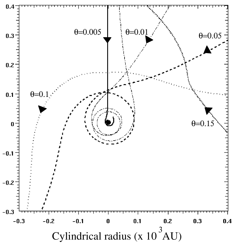
Figure 3: View down the axis of streamlines in the axial region for the virial-isothermal solution ($\alpha=-0.3$,$\Theta=0.41$). The streamline plotted with a solid line has the smallest angle with respect to the rotational axis. Other streamlines end with larger angles whose values are given for each streamline.

Fig.3 presents a zoom of streamlines in the axial region view from above . Streamlines start in the equatorial region and end in the axial region with small angles ($\theta=0.005$ to 0.15). In addition to the meridional behavior shown previously in Fig.2, each streamline makes a spiraling approach to the axis and then emerges in the form of an helix wrapped about the axis of symmetry. The closer in angle to the equator the streamline starts, the larger the angle of rotation it makes around the axis, the closer it gets to the central mass, and the nearer to the axis it asymptotically emerges. On the other hand, for streamlines beginning well above the equator, rotation is very nearly negligible and the path almost remains in a poloidal plane.

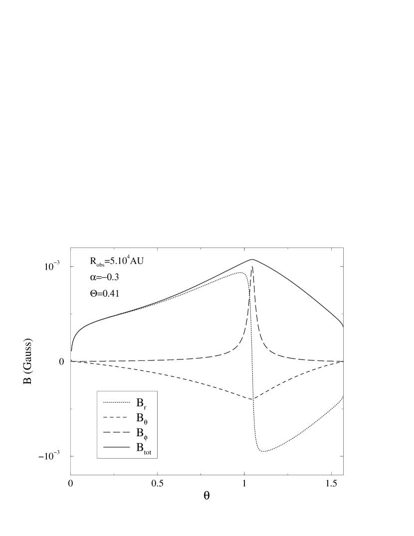
Figure 4: Virial-isothermal low mass solution: the angular dependence of magnetic field (in Gauss) at a distance of $5\times 10^{4}$ AU. Total magnetic field and $r$,$\theta$,$\phi$ components of $B$ are represented. ($\alpha=-0.3$,$\Theta=0.41$,$M\approx 1\leavevmode\nobreak\ M_{\odot}$)

Indirect measurements of the magnetic field in protostars are presently available (inferred from the radio flux from gyro-synchrotron emission by Ray et al. Ray (1997), and Hughes hughes (1999)). Such measurements can provide a critical test of models. In Fig.4 the angular dependences of the components of the magnetic field are shown in Gauss at a distance of $5\times 10^{4}$ AU for the same illustrative example of a low mass protostar. Magnetic fields of the order of a milligauss or less are obtained with a peak around 1 mGauss that coincides in angle with the radial turning point of the flow. As required by the quadrupolar geometry $B_{\phi}$ and $B_{\theta}$ vanish both on the equator and on the axis, while $B_{r}$ vanishes only on the axis and at the opening angle, where the largest field intensity exists.

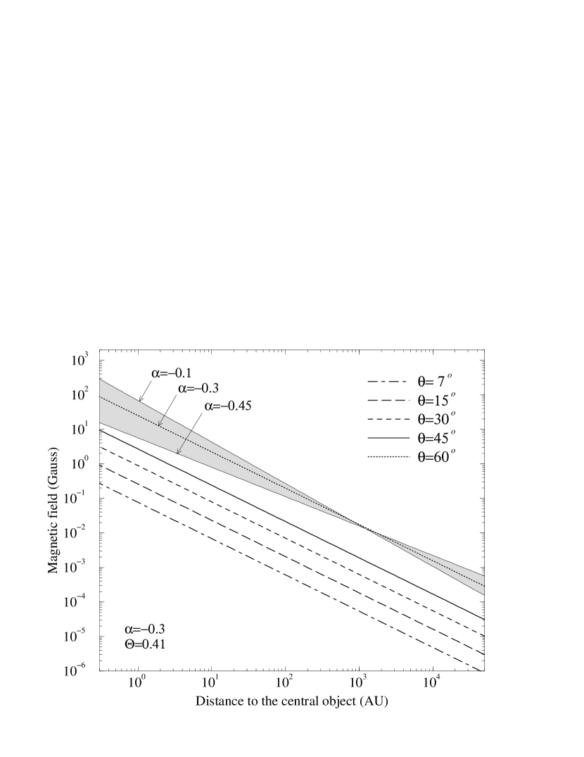
Figure 5: Virial-isothermal low mass solution ($\alpha=-0.3$,$\Theta=0.41$): magnetic field maximum (in Gauss) as a function of the distance to the central object (in AU) for different angles ($\theta=7,15,30,45,60$). The hashed region corresponds to the maximum magnetic field for different self-similar index ($\alpha=-0.45,-0.3,-0.1$,$M\approx 1\leavevmode\nobreak\ M_{\odot}$).

One remarkable prediction of these models is that the magnetic field at a given radius varies dramatically with angle (and hence probably with inclination to the line of sight). The values range from 10 microGauss to a milliGauss at $10^{4}$ AU, from $10^{-2}$ to a few Gauss at 20 to 40 AU in agreement with some observations (Ray et al. Ray (1997)). Peak field strengths may reach values as high as 1 to 100 Gauss at 1 AU (e.g. Hughes hughes (1999)), as shown in Fig.5. There is also a weaker dependence on the self-similar index as is also shown in Fig.5. These predicted magnetic field strengths are surprisingly large. This is nevertheless consistent with existing (rare) observations and reinforce the idea that magnetic fields play a major role around young stellar objects (Donati et al. donal97 (1997), Guenther & Emerson gue96 (1996)).

3.3 Massive Protostars

To adapt the model for high mass protostars, we must find solutions with higher self-similar density (according to Eq. 15) using the method outlined in Sect. 3.1 and adjust the other variables, mainly the magnetic field in fact, until the boundary conditions are satisfied. For radiative high mass protostars, we may speculate that we may not need a magnetic field as strong as in the low mass case to either launch or collimate the outflows since strong pressure gradients are produced by radiative heating (see also Shepherd & Churchwell shch (1996), Churchwell church (1997)). However the virial-isothermal model that we give below has a stronger magnetic field.

3.3.1 The Virial-Isothermal Case

Figure 6: Massive protostar virial-isothermal solution: Variations with angle of the self-similar variables (related to velocity ($u_{r}$, $u_{\theta}$, $u_{\phi}$), density ($\mu$ and $\mu_{a}$), magnetic field ($y_{p}$, $y_{\phi}$) and Mach number ($M_{ap}$, $M_{a\phi}$) with $\alpha=-0.1$,$\Theta=0.1$ (solid lines). The poloidal component $S_{p}$ of the Poynting flux is plotted in the lowest right panel. A low mass solution ($M\approx 1\leavevmode\nobreak\ M_{\odot}$) is plotted with dashed lines over the high mass case ($M\approx 30\leavevmode\nobreak\ M_{\odot}$).

Fig.6 shows the self-similar variables for a virial-isothermal massive object. This solution is also completely super-Alfvénic, just as is the previous low mass example that is overplotted with dashed lines. Although the overall opening angle of the flow (as measured by the angle at which the radial velocity changes sign) is the same in both cases, we observe that massive protostars produce faster (scaled) radial velocities throughout the positive range. There is also a more negative $u_{\theta}$ throughout this range which leads to an enhanced ‘collimation’, corresponding to an increased axial density of material. In addition, the peak rotation at the ‘turning point’ and the infall velocity just before this peak are both larger for the massive star. The smaller Alfvénic Mach numbers also show that the magnetic field is more important in this flow. This seems consistent with the ability to confine the higher physical temperature.

Our high mass virial-isothermal protostar yields larger scaled velocities than does the low mass object. This is mainly due to the larger luminosity in the high mass case. Sufficiently close to the axis both the low ($1\leavevmode\nobreak\ M_{\odot}$) and high ($30\leavevmode\nobreak\ M_{\odot}$) mass objects can produce $300\leavevmode\nobreak\ km\leavevmode\nobreak\ s^{-1}$. However as noted previously it is not clear that streamlines at such small angles are part of the present flow.

3.3.2 The Radiative Case

Massive molecular outflows present large bolometric luminosity, and therefore radiation probably plays an important role in the dynamics. Consequently radiative heating has to be investigated, taking into account consistently the diffusion equation. The radiation field and the temperature are no longer constant with angle and the radiation flux is not purely radial. The index $\alpha_{f}$ in Eq. 7 is chosen to be negative ($-0.1$ as in FH1) and so simulates a slight radiation loss. The numerical method is similar to that used above. The self-similar radiation flux $\@vec{f}(\theta)$ is fixed at $\theta_{min}$ to be zero , and the non-zero value at $\theta_{max}$ measures the radiation ‘loss’ from the self-similar region.

Figure 7: Massive protostar radiative solution: Variations with angle of the self-similar variables related to velocity ($u_{r}$, $u_{\theta}$, $u_{\phi}$), density ($\mu$ and $\mu_{a}$), radiation field ($f_{r}$, $f_{\theta}$), Mach number ($M_{ap}$) and temperature ($\Theta$) for $\alpha=-0.2$. $M\approx 5\leavevmode\nobreak\ M_{\odot}$.

Fig.7 shows a solution for the radiative case where $\alpha=-0.2$, $a=0$ and $b=2$. The temperature $\Theta$ is at its maximum (0.5) in the jet region and decreases towards the equator. The components of the radiation flux are much smaller than in FH1. Thus the required heating is less important than in FH1.

Fig.7 presents two illustrative radiative solutions for low ($M\approx 0.3\leavevmode\nobreak\ M_{\odot}$) and high mass ($M\approx 7\leavevmode\nobreak\ M_{\odot}$) cases. Streamlines in the poloidal plane are overplotted on contours of the hydrogen number density in the upper part of the figure, while the intensity of the radiation field is represented at the bottom. Fig.7 clearly shows the saddle type singularity of the central point. We see that a Keplerian disc naturally appears as part of the global solution as does the collimated outflow.

[[Caption of the figure that is given in gif format because of its size] Streamlines and density contours of the hydrogen number density (in logarithmic scale) for low and high mass radiative solutions with $\alpha=-0.2$. The density levels shown set between $10^{3}$ to $10^{5}$ cm^-3 for the low mass case, and between $10^{5}$ to $10^{7}$ cm^-3in the other case. Length scales are in AU. The lower panel presents the total intensity of the radiation field (on a logarithmic scale).]

The radiation field is smaller in the massive case in Fig.7. This is remarkable since one should expect significant radiative heating surrounding massive protostars. However, we have chosen to have the same components of the self-similar velocity for both cases, as well as the same self-similar temperature and radiation flux as input parameters. Therefore Fig.7 shows that the necessary radiation field has to be larger in low mass outflows in order to get the same scaled velocity as in the massive case. Particularly in the latter case, the global shape of the radiation field is rather similar to the solution obtained by Madej et al. (MLH (1987)), where an anisotropic radiation field was produced by scattering in thick accretion discs. It was shown in their article that collimation was clearly displayed by the radiation field in the polar region. We also find, in the massive case, that the radiation field increases away from the equator. On the other hand the low mass case almost shows an almost spherical symmetry, except on the axis.

Radiative heating increases the pressure gradient pushing outwards and therefore peak and asymptotic velocities along streamlines are larger as represented in Fig.8. This figure shows variation of total velocity with integrated distance along a streamline for both radiative and virial-isothermal cases for the same input parameters. We begin the integration in the equatorial region at about $10^{4}$ AU from the protostar and integrate out to $10^{6}$ AU in the axial region, where we attain a final angle of 0.1 radian (see FH1 for comparison). Velocity is maximum at the turning point ($u_{r}=0$), which is the closest point to the source, and is almost completely toroidal there. The inclusion of radiative heating provides a net acceleration of material which clearly increases the asymptotic axial velocity. Moreover the asymmetry in this graph indicates that the angular variation dominates the radial decrease as dictated by the self-similar forms. In fact this asymmetry is the clearest indication of the production of high velocity outflow from the relatively slow (but massive) infall.

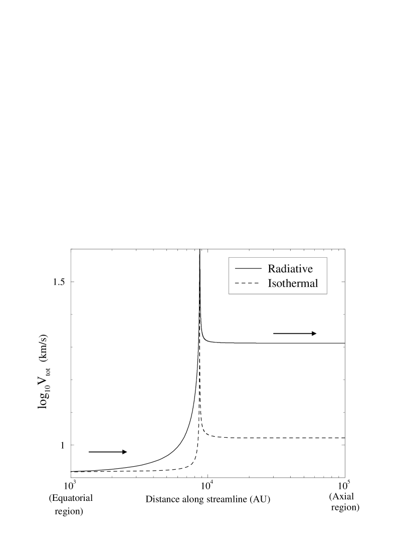
Figure 8: Variations of total velocity with integrated distance along a streamline for radiative (solid) and virial-isothermal (dashed) cases ($\alpha=-0.2$, $\Theta_{axis}=0.5$). The streamline are integrated from a radius of about $10^{4}$ AU in the equatorial region out to $10^{6}$ AU in the axial region, at a final angle of 0.1. The central object mass is $5\leavevmode\nobreak\ M_{\odot}$. Arrows denote the direction taken by the flow along streamline.

Global differences in the solutions between virial isothermal and radiative cases remain as described in FH1. The temperature is maximum in the jet region and decreases towards the equator. The radial component of the radiation flux decreases monotically in the same direction and its $\theta$-component increases, being always positive.

In order to show the influence of the mass on solutions, we present variations of the total velocity with the integrated distance along streamlines as defined in the previous plot for different masses in Fig.9. For all the curves, the input parameters are kept the same ($\alpha=-0.2$, $\Theta=0.5$) except for the mass of the central object and therefore the self-similar density $\mu$. Even the initial components of velocity and magnetic field remain the same. Only the starting distance of integration from the central object varies in order to differentiate the various curves. The larger luminosities for massive objects explain the larger velocities. In the solutions shown in Fig.9, the total velocity is multiplied by approximately a factor 5 as material flows from the equatorial region to the axial region. The efficiency of heating as a driving mechanism grows with the input values of the temperature $\Theta$ and of the components of the self-similar radiation flux $\@vec{f}$. Indeed, a factor of 10 or more can be obtained just by increasing these parameters. Moreover, the figure shows that the highest velocity components ($\approx\leavevmode\nobreak\ 100\leavevmode\nobreak\ km\leavevmode\nobreak\ s^{-1}$) are most tightly collimated along the axis ($\theta=0.02$). Thus the most massive protostars produce the fastest flows with maximum radial velocities in the axial region.

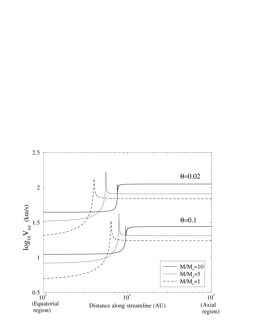
Figure 9: Variations of total velocity with integrated distance along a streamline for protostars of different masses. Solid lines represent a central object of 10 solar masses while dotted and dashed respectively stands for 5 and 1 $M_{\odot}$. Two sets of solutions are represented for two streamlines at different polar angles ($\theta=0.02;0.1$).

We conclude that radiative heating combined with Poynting flux driving provides an efficient mechanism for producing high velocity outflows when the opacity is dominated by dust.

3.4 Parameter Study

[[Caption of the figure that is given in gif format because of its size] Monte Carlo shooting: Plots of maxima of $u_{\phi}$ at the turning point ($u_{r}=0$) with respect to the maxima of $u_{\theta}$ for different values of the temperature parameter ($\Theta$=0.01;0.16;0.26;0.36). ($\alpha=-0.2$)]

We use a Monte Carlo exploration of our parameter space in order to study general trends in the model. The self-similar index and the temperature are fixed and the six input parameters (velocity and magnetic field scaled components and the density) are randomly chosen. The conditions presented in Sect. 3.1 are required for any solution to be considered ‘good’. One should note that there exists a broad range of solutions that possess favorable characteristics. Only the most significant results are reported here.

We plot the maxima of $u_{\phi}$ as functions of maxima of $u_{\theta}$ for various values of the self-similar temperature ($\Theta$=0.01;0.16;0.26;0.36), and for a given index ($\alpha=-0.2$). These maxima occur at the turning point where the radial velocity vanishes. Each point shown here represents a ‘good’ solution. Rotation is directly measured by $u_{\phi}$, and the tendency for material to go towards the axis, i.e. the collimation, is related to $u_{\theta}$. We find, as a global trend, that when $(u_{\theta})_{max}$ decreases, $(u_{\phi})_{max}$ remains almost constant ($(u_{\phi})_{max}\approx 0.25(u_{\theta})_{max}+constant$) until $(u_{\theta})_{max}$ reaches a threshold value. Then $(u_{\phi})_{max}$ decreases faster than $(u_{\theta})_{max}$, which is what was anticipated analytically for super-Alfvénic flow when $\alpha=1/4$ (see appendix B). In addition, there is a limiting $(u_{\phi})_{max}$ for each $(u_{\theta})_{max}$ at a given temperature, below which solutions are not found. When $\Theta$ increases, which physically corresponds to larger pressure gradients, $(u_{\phi})_{max}$ decreases while $(u_{\theta})_{max}$ becomes less negative. If the magnitude of the latter quantity is taken as a measure of the collimation, we see that rotation and collimation decrease together with increasing temperature and therefore probably with the bolometric luminosity of the central object.

It is found that solutions are less influenced by density (and hence mass) than by temperature. Nevertheless the distribution of opening angle is not found to change its form with temperature. In particular the most probable value is always found essentially at the angle shown in the two sample solutions. The variation is such that the larger opening angles are found at the lower left of the band for each temperature, that is with maximal poloidal collimation flow and the smallest possible maximum rotation.

It is also found that larger opening angles are associated with smaller magnetic fields. The corresponding results are not reported here, but in fact the variation of the opening angle is rather large for a relatively small magnetic field variation (a reduction of 25$\%$ in the magnetic field magnitude can widen the opening angle from $35^{\circ}$ to $60^{\circ}$). If the magnetic field varies secularly as the evolution proceeds, then a sequence of our models could be regarded as a series of ‘snapshots’ of the protostellar evolution. This evolutionary sequence would show that the opening angle increases with time, as the magnetic field becomes less important. This would be consistent with the notion that the youngest outflows are generally the most collimated. Indeed, this has been observationally verified by Velusamy and Langer (VeluLan (1998)), who provide evidence that outflows widen in time. Moreover when the magnetic field reaches a lower threshold in our model, the solution becomes a pure outflow. Therefore, as obtained with our model, if the opening angle broadens sufficiently, it may ultimately cut off the accretion supplying new material for the outflow.

Figure 10: The angular dependence of $u_{\theta}$ (left panel) and of density $\mu$ (right panel) for various self-similar temperature parameters (with $\alpha=-0.2$). Solutions with $\Theta=0;0.3;0.8$ are represented with solid lines. Two consecutive solutions are separated by a change of 0.1 in temperature.

The angular dependence of the self-similar variables are represented in Fig.10. The only parameter that varies is the self-similar temperature. The figure (left panel) illustrates the fact that collimation decreases with temperature as already mentioned. Moreover variations of the self-similar temperature give rise to different density profiles in the infalling ‘disc’ region, as seen on the right hand panel of Fig.10. The density decreases close to the equator for the largest values of the temperature with a maximum well away from the equator. Such solutions accrete so rapidly in the equatorial plane that they have a reduced density relative to their rotationally supported surroundings. These solutions resemble the special case $\alpha=1/4$ as discussed in appendix B. On the other hand the temperature has little effect on the density profile in the axial region, although it broadens the central ‘funnel’ substantially.

We note that solutions for cold flows ($\Theta=0$) have also been obtained. In such a case, the circulation is powered only by Poynting flux since our Bernoulli integral (Eq. 32) applies. We do not expect asymmetric velocities at the two infinities on the stream lines. For the same set of parameters, the total velocity in the ‘interacting’ region is smaller for cold flows and the fast rotating region (where $u_{\phi}$ is maximum) is narrower relative to finite pressure flows. Moreover the Alfvénic Mach numbers almost reach unity at the peak rotation point, showing that the flow is only slightly super-Alfvénic there, and that in fact the two terms in Eq. 32 are probably comparable.

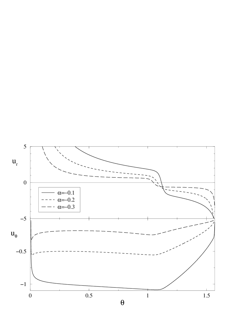
Figure 11: Dependences on the self-similar index $\alpha=-0.1,-0.2,-0.3$ (with $\Theta=0.3$). Radial (upper panel) and toroidal (lower panel) components of the self-similar velocity are plotted as functions of the angle.

Dependences of the self-similar index have also been investigated. The main results are illustrated by Fig.11 where the radial and longitudinal components of velocity are plotted for three values of the self-similar index but with the same self-similar temperature. For more negative self-similar index one gets dramatically smaller $\theta$- and $\phi$- velocities (recall that $\alpha=-1/2$ yields pure radial accretion) and a smaller change in the radial velocity.

4 Observational Consequences of the Model: Synthetic ${}^{13}CO$ Spectral Lines and Maps.

In this Section, we compute ${}^{13}CO$ (J=$1\rightarrow 0$) emission lines for several of the outflow solutions discussed in Sect. 3.1. Specifically, we provide examples of spectra, channel maps, position-velocity diagrams, and intensity-velocity diagrams for one example of each of the following: the low mass solution of Sect. 3.2, the radiative high mass solution of Sect. 3.3.2, and the virial-isothermal high mass solution of Sect. 3.3.1. The importance of this analysis is that it allows us to directly compare the observable features of our models with real observational data. However, we cannot fully explore the observational consequences of our models in the present paper. Our purpose in this Section will be mainly to outline the qualitative features of our models, leaving a complete exploration of the parameter space for the second paper in our series.

The method that we follow is essentially the same as that outlined in FH2, except that the code used there has been substantially improved in a number of respects. Firstly, we are now able to generate results with much higher spectral and spatial resolution. Secondly, although we compute spectra on a grid of pencil beams through the outflow source, we convolve our spectra with a Gaussian telescope beam to more accurately simulate observational results. FH2, on the other hand, did not perform this convolution, which resulted in many spuriously sharp features in their maps. Thirdly, we do not embed our solutions in a background of molecular gas to simulate the molecular cloud, which presumably surrounds the outflow. FH2 demonstrated that the presence of background material has no significant effect on the spectra or maps, except for in the lowest, and hence least interesting, velocity channels. Since we are primarily interested in emission at relatively high velocities, corresponding to the outflow, emission or absorption by relatively slow moving background gas is of no consequence. As in FH2, the primary limitation of our analysis is that we assume local thermodynamic equilibrium. Although this is probably not strictly true, we do expect the ${}^{13}CO$ level populations to be approximately in equilibrium with the local temperature provided that the optical depth is at least moderately high. Therefore, we hope to capture at least the character of the emission, if not the precise intensity.

4.1 Low Mass Solutions

We have assumed a mass of $1\leavevmode\nobreak\ M_{\odot}$ for the low mass solution, which implies a fiducial radius of $r_{o}=1400\leavevmode\nobreak\ AU$ using Eq. 13. We have also chosen a inclination angle of $45^{\circ}$ between the symmetry axis of the outflow and the plane of the sky. With the mass and $r_{o}$ determined, the density, temperature, and velocity are determined at any position by the dimensionless parameters $\mu(\theta)$ and $\Theta(\theta)$, and the radial scalings given by Eqs. 1-7. Therefore, by constructing a line of sight through the cloud, we can compute the emission (expressed as a radiation temperature) as a function of velocity parallel to the line of sight; examples of these spectra are shown in Fig.12. We have computed spectra on a $61\times 120$ grid of map positions across the outflow.

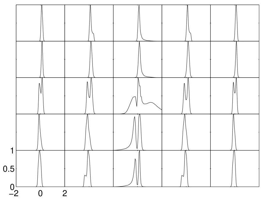
Figure 12: Normalized spectra are shown for the low mass solution on a $5\times 5$ grid of map positions that are evenly spaced across the mapped region, which is $20\times 40\leavevmode\nobreak\ r_{o}$ in size. The abscissa is in units of $km\leavevmode\nobreak\ s^{-1}$. The source is located at the center.

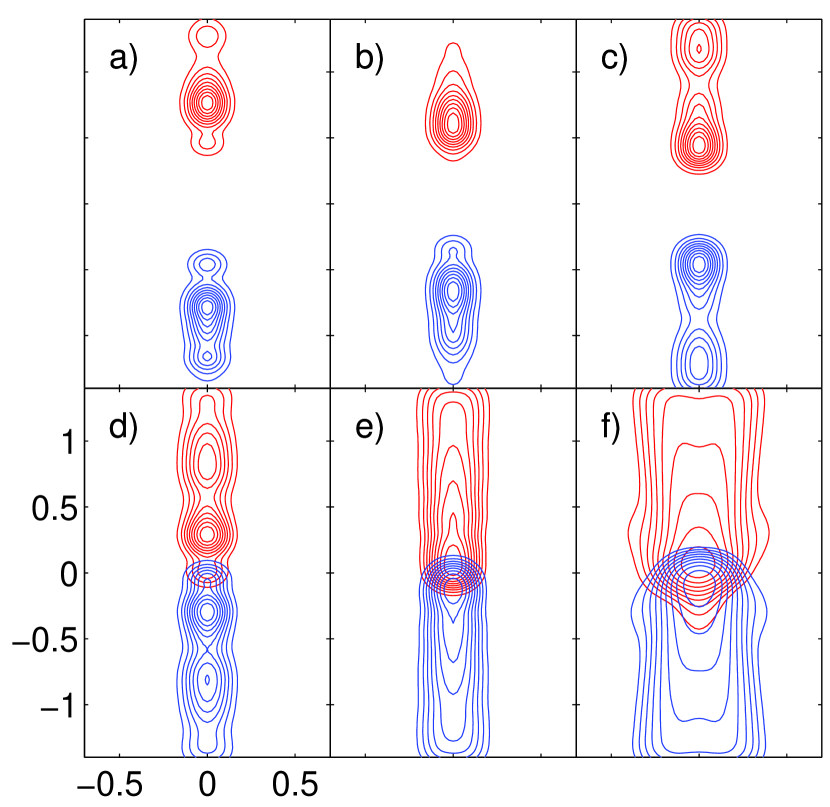
Figure 13: Channel maps for the low mass solution at an inclination angle of $45^{\circ}$. In units of $km\leavevmode\nobreak\ s^{-1}$, the velocity channels are as follows for panels a) through f): a) $5.5<|v|<6.5$, b) $4.5<|v|<5.5$, c) $3.5<|v|<4.5$, d) $2.5<|v|<3.5$, e) $1.5<|v|<2.5$, f) $0.5<|v|<1.5$. The upper part of the outflow is the red-shifted side, while the lower part is blue-shifted. Map coordinates are in units of $10^{4}\leavevmode\nobreak\ AU$.

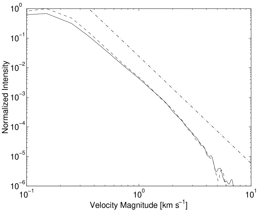
Figure 14: Intensity-velocity diagram for the low mass solution. The dot-dashed line represents a power-law fit with an index of $-3.5$.

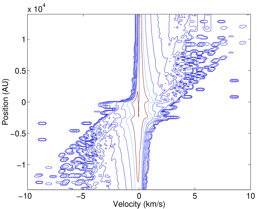
Figure 15: Position-velocity diagram for the low mass solution.

We find that the spectra shown in Fig.12 vary substantially with map position across the outflow. Spectra computed near the map projection of the outflow axis typically show relatively high velocity wings that may extend up to several $km\leavevmode\nobreak\ s^{-1}$, but the emission generally becomes too weak to show past $\approx 2\leavevmode\nobreak\ km\leavevmode\nobreak\ s^{-1}$. We note that the strongest emission always occurs at low velocities, with relatively weak emission in the wings, as is the case for real outflows. Spectra may contain either a single wing or both red and blue-shifted wings depending on whether a particular line of sight crosses only a single lobe of the outflow or both. There are also many cases where line wings are absent, but well-defined “shoulders” are present on the low velocity dominated spectra.

In the equatorial regions of the maps, double-peaked spectra are found with relatively low velocity peaks. These spectra are mainly due to the radial infall that dominates in the equatorial regions. It is unlikely that the double-peaked profiles are due to rotation, since radial infall velocities exceed the rotational velocities at all angles $\theta$ except for very near the radial turning point of the outflow. Furthermore, many of the spectra have a slight asymmetry in which the blue-shifted peak shows stronger emission. This is suggestive of the well-known outflow asymmetry, which is due to the more efficient self-absorption of blue-shifted emission by overlying material moving towards the observer (Shepherd & Churchwell shch (1996), Gregersen et al. greg (1997), Zhou et al. zhou (1996)). The effect is slight in this case since the low mass solution, with a $1\leavevmode\nobreak\ M_{\odot}$ central object, produces a peak optical depth of only $\approx 0.2$ along most lines of sight. The massive solutions, discussed in Sect. 3.3.2 and 3.3.1, produces much higher optical depths and leads to a much more pronounced asymmetry.

Fig.13 shows a set of channel maps for the low mass solution. To make these synthetic maps, we have integrated the emission over $1\leavevmode\nobreak\ km\leavevmode\nobreak\ s^{-1}$ wide channels from $-6.5$ to $6.5\leavevmode\nobreak\ km\leavevmode\nobreak\ s^{-1}$. We have deliberately excluded the emission with $|v|<1\leavevmode\nobreak\ km\leavevmode\nobreak\ s^{-1}$, since we find that the lowest velocity emission is essentially featureless. We have convolved the maps with a Gaussian telescope beam with a FWHM of $800\leavevmode\nobreak\ AU$; for example, this corresponds to a $5\leavevmode\nobreak\ arcsec$ beam at a distance of $160\leavevmode\nobreak\ pc$.

The outflow is apparent at all velocities shown in our maps. We obtain a relatively wide outflow “cone” at the lowest velocities ($0.5$ to $1.5\leavevmode\nobreak\ km\leavevmode\nobreak\ s^{-1}$) and very well collimated jet-like emission apparent at velocities between $1.5$ and $3.5\leavevmode\nobreak\ km\leavevmode\nobreak\ s^{-1}$. At higher velocities, the jet-like feature breaks up into outflow “spots” that move away from the central object as the velocity increases. The most important feature of these channel maps is that the opening angle of the outflow gradually decreases as the magnitude of the velocity increases. As discussed in FH2, this effect is entirely due to the angular velocity sorting of the outflow solutions. Our models always have the property that the outflow velocity increases towards the axis of symmetry. Thus, our models naturally produce outflows in which most of the material is poorly collimated and moves at relatively low velocities, but the fastest jet-like components are very well collimated towards the axis of symmetry. This property has, in fact, been observed in a number of outflow sources (Bachiller et al. bachiller (1990), Guilloteau et al. Guilloteau (1992), Gueth et al Gueth (1996)).

Several authors have noted that molecular outflows seem to be characterized by a power-law dependence of total integrated intensity as a function of velocity (Rodriguez et al. Rodriguez (1982), Masson & Chernin Masson (1992), Chandler et al. Chandler (1996)). In Fig.14, we have summed all of the spectra in order to show how the intensity is distributed with velocity. The solid line in the figure represents the blue-shifted emission, while the dashed line represents the red-shifted emission. We note that there are no important differences due to the somewhat low optical depth of our solution. We find that the intensity $I$ is well fit by a power law $I\propto v^{-3.5}$ over all velocities greater than approximately $0.2\leavevmode\nobreak\ km\leavevmode\nobreak\ s^{-1}$. This power-law behavior has, in fact, been found for several real outflows , and the index is in reasonable agreement with the available data (Cabrit et al. cab (1996), and Richer et al. PPIV (1998)). It remains to be seen, however, how sensitive the power-law index is to the parameters of our model. This important issue will be resolved in the second paper in this series, where we more completely explore the line emission of our models.

An important feature of Fig.14 is that the emission falls very rapidly with increasing velocity. For example, the intensity at even a rather modest velocity of $3\leavevmode\nobreak\ km\leavevmode\nobreak\ s^{-1}$ is only $0.01\%$ of the peak intensity. At some velocity, the emission will fall below the noise threshold that is always present in real observations. Past this velocity, the emission shown in Fig.13 would be undetectable.

In Fig.15, we show a velocity-position diagram for a cut along the outflow axis. We have actually computed spectra along several cuts parallel to the outflow axis and convolved them with a Gaussian beam to produce a single velocity-position diagram. We find that there is substantial emission at low velocities along the entire cut. The highest velocities are found near the map centre, as must be the case since $v\propto r^{-1/2}$ by Eq. 1. We note that the emission contours in this figure are logarithmically spaced; thus, we find that the most intense emission occurs at low velocities at all map positions.

The outflow is apparent in Fig.15 by the emission extending out to approximately $\pm 8\leavevmode\nobreak\ km\leavevmode\nobreak\ s^{-1}$ on either side of the outflow. Moreover, the general appearance of the position-velocity diagram is suggestive of a globally accelerated flow since higher velocities generally appear at greater distances from the central source. How can this be reconciled with the fact that velocity decreases with radius in our model? It was shown in FH2 that the apparent acceleration is due to the unique velocity sorting that is predicted by our model. The radial velocity always increases with decreasing polar angle near the outflow axis. Our cut crosses progressively smaller angles with increasing distance from the central object, and therefore encounters higher velocity material.

The ragged appearance of the highest velocity contours is entirely due to the limitations of our numerical procedures at high velocities. In our model, the highest velocity components are extremely localized near the central star and the outflow axis. Thus, whether or not a pencil beam passes through such a component is a matter of chance when the spatial extent falls below the grid spacing. This apparently happens when $|v|\gtrsim 5\leavevmode\nobreak\ km\leavevmode\nobreak\ s^{-1}$.

4.2 Massive Solutions

4.2.1 The Radiative Case

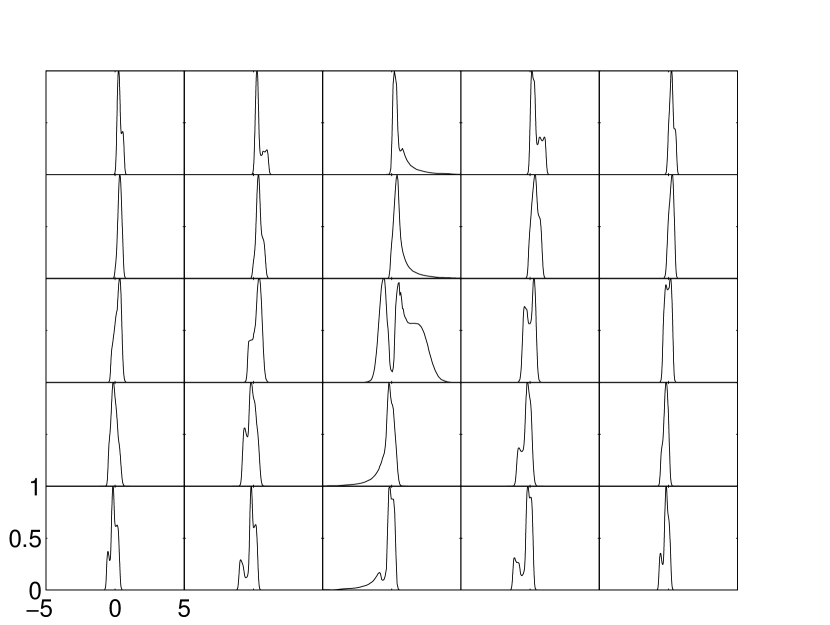
Figure 16: Normalized spectra are shown for the radiative solution on a $5\times 5$ grid of map positions that are evenly spaced across the mapped region, which is $10\times 20\leavevmode\nobreak\ r_{o}$ in size. The abscissa is in units of $km\leavevmode\nobreak\ s^{-1}$.

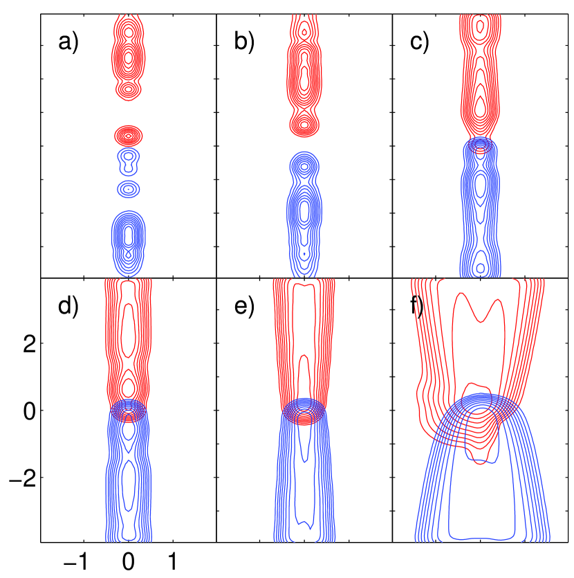
Figure 17: Channel maps for the radiative solution at an inclination angle of $45^{\circ}$. In units of $km\leavevmode\nobreak\ s^{-1}$, the velocity channels are as follows for panels a) through f): a) $11<|v|<13$, b) $9<|v|<11$, c) $7<|v|<9$, d) $5<|v|<7$, e) $3<|v|<5$, f) $1<|v|<3$. The upper part of the outflow is the red-shifted side, while the lower part is blue-shifted. Map coordinates are in units of $10^{4}\leavevmode\nobreak\ AU$.

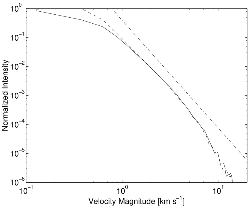
Figure 18: Intensity-velocity diagram for the radiative solution. The dot-dashed line represents a power-law fit with an index of $-3.6$.

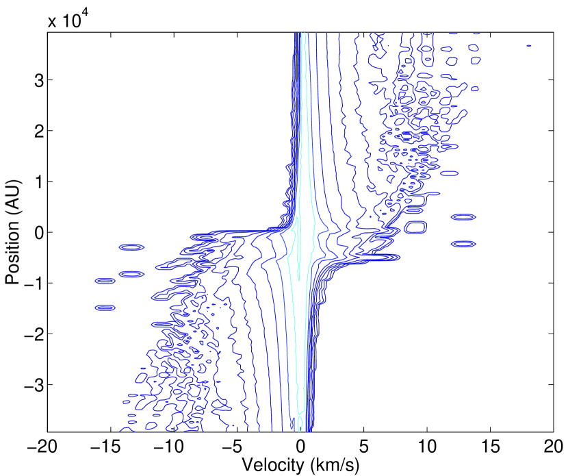
Figure 19: Position-velocity diagram for the radiative solution.

It is useful to compare the ${}^{13}CO$ emission of the radiative solution discussed in Sect. 3.3.2, with the low mass solution discussed above. We have assumed a mass of $10\leavevmode\nobreak\ M_{\odot}$, which implies a fiducial radius of $r_{o}=7900\leavevmode\nobreak\ AU$ according to Eq. 13. We find, heuristically, that the peak optical depth in the line centre decreases with increasing central mass. Since the mass is a free parameter, we have tuned it to achieve realistic optical depths of order unity. The mass is larger than for the low mass solution discussed above, but the effects of radiative heating are more likely to become important in outflows surrounding more massive protostars, in any case. The only other parameter that we have changed is the FWHM of the Gaussian beam that we convolve with our solution; here, we can use a slightly larger and more realistic 10 arcsec beam without smearing out the details of the solution. As in Sect. 4.1, we have computed spectra on a $61\times 120$ grid of map positions assumed a $45^{\circ}$ inclination angle.

Qualitatively, we find a great deal of similarity with the low mass solution. The line profiles shown in Fig.16 have similar structure, and the outflow shown in Fig.17 is collimated to a similar degree. The main difference is the velocity of the flow. In the radiative case, we find that there is significant emission out to at least $10\leavevmode\nobreak\ km\leavevmode\nobreak\ s^{-1}$, and we find some low intensity emission out to $15\leavevmode\nobreak\ km\leavevmode\nobreak\ s^{-1}$; this is most clearly illustrated by the position velocity diagram shown in Fig.19. Examining the intensity-velocity diagram shown in Fig.18, we find that the intensity $I\propto v^{-3.6}$ for velocities greater than about $0.5\leavevmode\nobreak\ km\leavevmode\nobreak\ s^{-1}$. It is striking that nearly the same power law index should be obtained for both the low mass and radiative solutions. Admittedly, we do not fully understand the reasons for this similarity in behavior at present. We also doubt that this sort of behavior is a generic feature of our models. Nevertheless, we are encouraged that at least some of our models are capable of reproducing such realistic observed properties.

4.2.2 The Virial-Isothermal Case

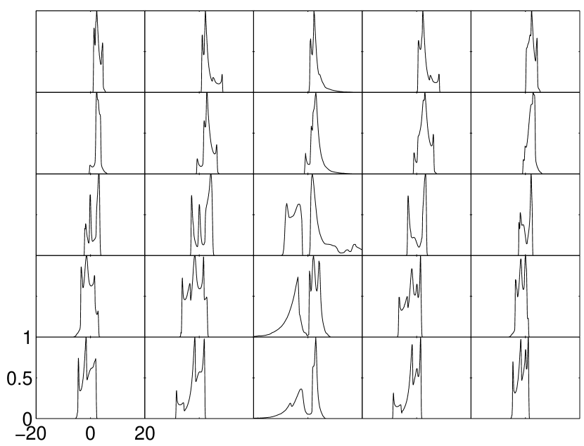
Figure 20: Normalized spectra are shown for the massive solution on a $5\times 5$ grid of map positions that are evenly spaced across the mapped region, which is $2.5\times 5\leavevmode\nobreak\ r_{o}$ in size. The abscissa is in units of $km\leavevmode\nobreak\ s^{-1}$.

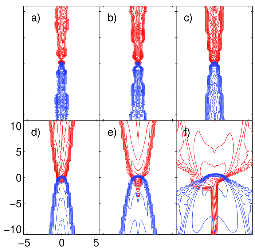
Figure 21: Channel maps for the massive solution at an inclination angle of $45^{\circ}$. In units of $km\leavevmode\nobreak\ s^{-1}$, the velocity channels are as follows for panels a) through f): a) $30<|v|<35$, b) $25<|v|<30$, c) $20<|v|<25$, d) $15<|v|<20$, e) $10<|v|<15$, f) $5<|v|<10$. The upper part of the outflow is the red-shifted side, while the lower part is blue-shifted. Map coordinates are in units of $10^{4}\leavevmode\nobreak\ AU$.

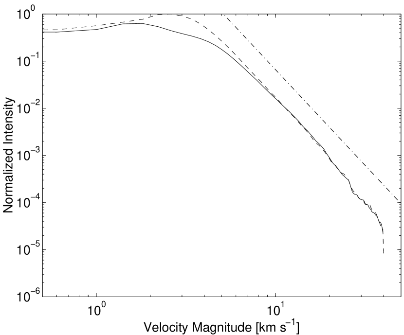
Figure 22: Intensity-velocity diagram for the massive solution. The dot-dashed line represents a power-law fit with an index of $-4.1$.

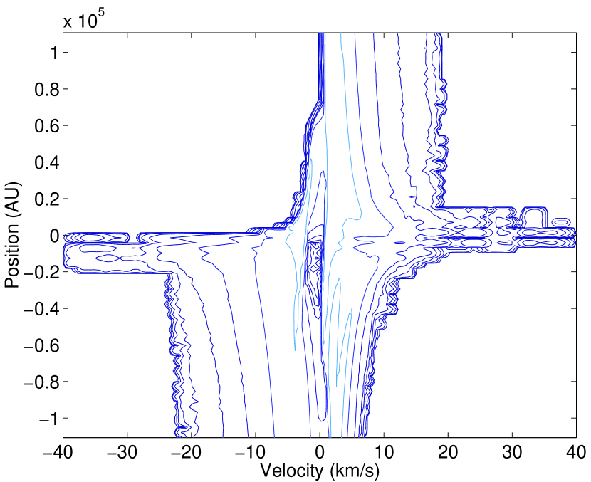
Figure 23: Position-velocity diagram for the massive solution.

We have also computed the ${}^{13}CO$ emission of the high mass solution discussed previously in Sect. 3.3.1. We find that the optical depth is extremely high unless the mass of the central protostar is chosen to be rather large; therefore, we have used a mass of $100\leavevmode\nobreak\ M_{\odot}$ and a corresponding fiducial radius of $r_{o}=44000\leavevmode\nobreak\ AU$ to compute the spectra. Even using such a large central mass, we find that the peak optical depth in the line centre is very high, with values exceeding 5 in many positions. Such high optical depths cause real difficulty for the present version of our code, since any given line of sight encounters the “photosphere”, where the optical depth at some velocity is approximately unity, rather abruptly. Thus, a great deal of care was taken to ensure that the solution was well-sampled along each line of sight. We note that the corresponding increase in computational time required us to decrease the spatial resolution of our maps. Here, we employ a $41\times 80$ grid, as opposed to the $61\times 120$ grid used elsewhere. The inclination angle is $45^{\circ}$, as in the previous two cases.

The spectra shown in Fig.20 are much more complex than the spectra of the low mass or radiative solutions. Many show multiple sharp peaks and very extended wing emission out to well past $20\leavevmode\nobreak\ km\leavevmode\nobreak\ s^{-1}$ (as in Shepherd & Churchwell shch (1996), Gregersen et al. greg (1997) for CO maps of molecular outflows, and Doeleman et al. doeleman (1999) for SiO masers). We are quite certain that the multiple peaks are real, and not numerical artifacts, since we have verified that their location and appearance is independent of the spectral resolution and the degree to which a solution is sampled along a line of sight. It remains unclear to us in detail why such jagged peaks should be present, although it must depend on the variation of optical depth, density and velocity field within the ‘beam’. Thus behavior should be studied as a function of inclination to the line of sight.

Despite the unusual appearance of the spectra, the channel maps shown in Fig.21 are quite reasonable. A well-collimated outflow is apparent at velocities greater than about $10\leavevmode\nobreak\ km\leavevmode\nobreak\ s^{-1}$. The position velocity diagram shown in Fig.23 shows significant emission at most positions out to approximately $20\leavevmode\nobreak\ km\leavevmode\nobreak\ s^{-1}$. We obtain emission at higher velocities (up to approximately $40\leavevmode\nobreak\ km\leavevmode\nobreak\ s^{-1}$, but the emission is restricted to the central map positions nearest the protostar. The intensity-velocity diagram (Fig.22) again shows a power law behavior, but the slope is different than that obtained in the previous two cases; here we find that $I\propto v^{-4.1}$, which is still inside the range allowed by the available observations (Cabrit et al. cab (1996), Richer et al. PPIV (1998)).

5 Discussion

5.1 The Alfvénic Point

Figure 24: We show the density $\mu$ and the Alfvénic density $\mu_{a}$ for really super Alfvénic (upper panel), slightly super Alfvénic in the region of naught radial velocity (middle panel) and critical (lower panel) solutions. From top to bottom Poynting flux and radial velocity are getting less and less important ($\alpha=-0.2$,$\Theta=0.41$).

All the solutions presented previously were completely super-Alfvénic. Here we report a trans-Alfvénic solution in order to show why they are generally not preferred. In such a solution, the outflow size is reduced and the ultimate velocities are smaller. Therefore this type of solution is less efficient in producing high velocity outflows. Entirely sub-Alfvénic solutions can also be found but they admit only pure accretion. Fig.24 shows the density profile for two super-Alfvénic solutions (the two upper most plots A and B) and one trans-Alfvénic solution (C). Case (A) presents a model where the density is well above the critical Alfvénic density. In this case, the Alfvénic Mach number is larger than unity. The second case (B) has almost the critical density at the turning point, and consequently the Alfvénic Mach number almost reaches unity at this point. However the solution always remains super-Alfvénic. Finally the lower panel (case C) displays a trans-Alfvénic solution showing that the size of the outflow has been reduced drastically. Therefore the most interesting solutions for circulation flow appear to be super-Alfvénic solutions.

5.2 Comparison with FH1

Figure 25: Comparison of streamlines without Poynting flux (dashed line) and including Poynting flux (solid line) starting from the same position in the equatorial plane. ($\alpha=-0.3$,$\Theta=0.41$)

Fiege & Henriksen (fiege1 (1996)a, FH1) have shown that $r$-self-similar quadrupolar circulation could be a relatively realistic model for bipolar outflow. They did not include Poynting flux that could assist the outflow as in the present paper. The inclusion of this effect allows us to obtain faster and more collimated outflows. The path followed by material also differs from FH1 as shown in Fig.25, where streamlines from FH1 and the present models are plotted. All the solutions start from approximately the same initial position in the equatorial region with the same set of parameters. Streamlines from the present model get closer to the source than the FH1 solution, for both radiative and virial-isothermal cases. Thus, in the present model, the flow passes relatively close to the central mass. The limiting speed is about the escape speed from the central mass (and the jet speed) of a few hundred $km\leavevmode\nobreak\ s^{-1}$. We note that the most collimated of the the three solutions is the radiative case.

5.3 Stability Analysis

The steady configurations presented in this article should develop strong shocks in the axial region due to the strong collimation created by magnetic and pressure forces. Moreover current-carrying jets, as in the present model, are liable to Kelvin-Helmholtz (KH), Pressure Driven (PD) and magnetic instabilities driven by the electrical current. These so called current driven (CD) instabilities have been studied only recently in the context of astrophysical jets (Appl appl (1996), Appl et al. LBA (1999)). We use the results of the latter linear stability analysis in order to get a rough estimate of CDI and KHI in our magnetic configuration. Growth rates $\Gamma$ of the different modes show that the CD helical mode ($m=1$) dominates the CD pinching mode ($m=0$) and that CD and KH instabilities become comparable when the Mach number approaches unity. This is the case in the present self-similar model. The CD instability (with a typical wavelength $\lambda_{CD}\approx\frac{2}{5}R_{outflow}$, $R_{outflow}$ being the characteristic size of the outflow) should be located on a current sheet where reconnection and particle acceleration might occur. KH pinching modes ($\lambda_{KH}\approx 3\times R_{outflow}$) should dominate KH helical modes, and consequently give rise to internal shocks in the outflow. All these results require numerical simulations that we plan to study in another paper.

6 Conclusions

In this paper we have presented a model based on the $r$-self-similarity assumption applied to the basic equations of ideal axisymmetric and stationary MHD, including Poynting flux. Detailed comparisons with the observations have been computed and characteristic scales of the problem have been given as functions of source properties. The luminosity needed for radiative heating is smaller even while driving faster outflows than in the previous model (FH1). The model geometry implies a natural connection between the fast ionized jets seen near the polar axis of the wind, and the slower and less-collimated molecular outflows that surround them, although the jets may be partly due to central activity not included in our model.

The most massive protostars produce the fastest flows with maximum radial velocities in the axial region. Radiative heating produces faster outflows compared to the virial-isothermal case, for both low and high mass objects. Larger opening angles are associated with smaller magnetic fields. Consequently, a gradual evolutionary loss of magnetic flux may result in outflows that widen as they age.

Synthetic spectral lines from ${}^{13}CO$ (J=$1\rightarrow 0$) allow direct comparison with observational results via channel maps, maps of total emission, position-velocity and intensity-velocity diagrams. The model reproduces well observational features. Due to internal instabilities in the most collimated ‘jet’ part of the flow, the time evolution of the steady model should give rise to regularly spaced knots, and possibly excitation, ionization and non-thermal particle acceleration due to field annihilation and shock dissipation. Thus the model in its current state of development shows that radiative heating combined with Poynting flux driving is efficient in producing high velocity outflows when the characteristic luminosity of the forming star (as deduced from observations) is used. More extensive searches in parameter space, the detailed fit to specific sources, and time dependent modeling all remain to be done. Although we do not discuss the regions excluded from the self-similar region of the flow, the current correspondence to observational features is sufficiently exact that we expect simultaneous infall/outflow (‘circulation’) to be an essential part of any realistic model.

Appendix A The Equations

The mass flux conservation equation remains the same as in FH1:

$$\left(1+2\,\alpha\right)\mu\,u_{{r}}+\frac{1}{\sin{\theta}}\frac{d}{d\theta}\left(\mu\,u_{\theta}\sin{\theta}\right)=0,$$ (33)

while the self-similar variable $y$ is simply replaced by its poloidal component in the following set of equations:

Magnetic Flux conservation:

$${\frac{\left(\alpha+5/4\right)u_{{r}}}{y_{{p}}}}+\frac{1}{\sin{\theta}}{\frac{d}{d\theta}}\left({\frac{u_{\theta}\sin{\theta}}{y_{{p}}}}\right)=0$$ (34)

Radial component of momentum equation:

$$u_{\theta}\frac{du_{r}}{d\theta}\left(1-{M_{{ap}}}^{-2}\right)-\left({u_{\theta}}^{2}+{u_{\phi}}^{2}\right)\left(1-{\frac{\alpha+1/4}{M_{ap}^{2}}}\right)$$

$$-\frac{u_{r}^{2}}{2}-\left(\frac{3}{2}-2\alpha\right)\Theta+1+\frac{u_{r}u_{\theta}}{M_{ap}^{2}y_{p}}\frac{dy_{p}}{d\theta}=0$$ (35)

Other equations of the system contain terms with mixed toroidal and poloidal components; Angular Momentum conservation:

$$\frac{1}{u_{\phi}}{\frac{du_{\phi}}{d\theta}}\left(1-\frac{1}{M_{ap}M_{a\phi}}\right)+\frac{u_{r}}{u_{\theta}}\left(1/2-{\frac{\alpha+1/4}{M_{ap}M_{a\phi}}}\right)$$

$$+\cot\leavevmode\nobreak\ \theta\left(1-{\frac{1}{M_{{ap}}M_{{a\phi}}}}\right)+{\frac{1}{y_{{\phi}}M_{{ap}}M_{{a\phi}}}}{\frac{dy_{\phi}}{d\theta}}=0$$ (36)

Faraday’s law plus zero comoving electric field:

$${\frac{d(u_{{\phi}}u_{{\theta}})}{d\theta}}+\left[\alpha-\frac{1}{4}\right]u_{{\phi}}u_{{r}}+u_{{\phi}}u_{{\theta}}{\frac{d}{d\theta}}\ln\left[\frac{1}{y_{{p}}}-\frac{1}{y_{{\phi}}}\right]=0$$ (37)

$\theta$-component of momentum equation:

$$\frac{u_{r}u_{\theta}}{2}\left(1-{\frac{2\,\alpha+1/2}{{M_{ap}}^{2}}}\right)+{u_{\phi}}^{2}\cot\leavevmode\nobreak\ \theta\left({M_{a\phi}}^{-2}-1\right)$$

$$+{\frac{u_{r}}{{M_{ap}}^{2}}}{\frac{du_{r}}{d\theta}}+u_{\theta}{\frac{du_{\theta}}{d\theta}}+{\frac{u_{\phi}}{M_{ap}^{2}}}{\frac{du_{\phi}}{d\theta}}-{\frac{{u_{r}}^{2}}{{y_{p}M_{ap}}^{2}}}{\frac{dy_{p}}{d\theta}}$$

$$-{\frac{{u_{\phi}}^{2}}{{y_{\phi}M_{a\phi}}^{2}}}{\frac{dy_{\phi}}{d\theta}}+{\frac{d\Theta}{d\theta}}+{\frac{\Theta}{\mu}}{\frac{d\mu}{d\theta}}=0$$ (38)

To treat the radiative heating we either hold $\Theta$ constant (virial-isothermal case) as discussed above, or we include the equations of radiative diffusion (radiative case) as in FH1. The equations (17), (18) and (22) of FH1 continue to apply provided that the optical depth given above is $\geq 2/3$.

Appendix B The First integrals

Equations (33) and (34) together yield the first integral

$$\mu(u_{\theta}\sin{\theta})^{\frac{1/4-\alpha}{5/4+\alpha}}y_{p}^{\frac{1+2\alpha}{5/4+\alpha}}\equiv q_{1}/4\pi,$$ (39)

where $y_{p}$ replaces $y$ in FH1. Moreover directly from Eq. 33 and the poloidal stream-line equation $dr/rd\theta=u_{r}/u_{\theta}$ we have the stream-line integral

$$r^{(1+2\alpha)}\mu u_{\theta}\sin{\theta}\equiv\eta_{1}.$$ (40)

From this we see immediately that $\alpha>-1/2$ if we are to have quadrupolar stream-lines for which $r\leavevmode\nobreak\ \rightarrow\leavevmode\nobreak\ \infty$ as $u_{\theta}\leavevmode\nobreak\ \rightarrow\leavevmode\nobreak\ 0$. A second stream-line integral follows from Eq. 34 and the stream-line equation, but it is not independent of Eqs. 39 and 40 since it follows by eliminating $\mu$ between these two. The limit $\alpha<1/4$ follows immediately from Eq. 39 if we require finite $\mu$, $u_{\theta}=0$ and odd symmetry in the magnetic field at the equator. The integral then implies implies that $y_{p}\rightarrow\infty$ and so the field passes through zero in the equatorial plane. This conclusion is avoided on the polar axis since the radial velocity is free to become very large there. This choice has the additional merit that the equator is super Alfvénic as well as the axis.

Using Eq. 34 together with Faraday’s law (37) we obtain the integral

$$u_{\phi}\left[\frac{1}{y_{p}}-\frac{1}{y_{\phi}}\right]\left(\frac{\sin{\theta}}{y_{p}}\right)^{\frac{1/4-\alpha}{5/4+\alpha}}u_{\theta}^{\frac{3}{2(5/4+\alpha)}}=q_{2}.$$ (41)

Note that the constant $q_{2}$ is very interesting because it can be used to measure the strength of the electric field which is in fact

$$\@vec{E}=-\left[\frac{GM}{cr_{o}}\right]\sqrt{\frac{M}{r_{o}^{3}}}\left(\frac{r}{r_{o}}\right)^{\alpha-\frac{5}{4}}\left[\frac{1}{y_{p}}-\frac{1}{y_{\phi}}\right]\left(\@vec{u_{\phi}}\times\@vec{u_{p}}\right).$$ (42)

The integral is not present in FH1 since the electric field is everywhere zero there.

In general we can not find an angular momentum integral explicitly (this is related to the difficulty of expressing scale invariance in an action principle; B. Gaffet, private communication) but in the special case of similarity index $\alpha=1/4$ such an explicit integral exists in the form (cf FH1):

$$\frac{u_{\theta}\sin{\theta}}{M_{ap}^{2}}\equiv q_{3}\left(u_{\phi}\sin{\theta}\right)^{3}\left(1-\frac{1}{M_{ap}M_{a\phi}}\right)^{3}.$$ (43)

Although this is a very special case not normally related to our numerical solutions (the mass density is constant in radius so that eventually the dominance of the central mass is broken as $r$ increases), it is instructive to consider it further. Eq. 39 becomes simply $\mu=(q_{1}/4\pi)y_{p}^{-1}$ so that $M_{ap}^{2}=q_{1}y_{p}$ and $M_{a\phi}^{2}=q_{1}y_{\phi}^{2}/y_{p}$. Then Eqs. 41 and 43 can be solved together for $y_{p}$ and $y_{\phi}$ to give

$$\frac{1}{y_{p}}=\frac{q_{2}q_{3}\sin^{2}{\theta}+q_{1}q_{3}u_{\phi}u_{\theta}\sin^{2}{\theta}}{q_{3}u_{\phi}u_{\theta}\sin^{2}{\theta}+u_{\theta}^{2}/u_{\phi}^{2}},$$ (44)

and

$$\frac{1}{y_{\phi}}=\frac{q_{1}q_{3}u_{\phi}^{4}\sin^{2}{\theta}-q_{2}}{q_{3}u_{\phi}^{4}\sin^{2}{\theta}+u_{\phi}u_{\theta}}.$$ (45)

We therefore observe that near the equator $y_{p}$ can be infinite only if $u_{\phi}\rightarrow 0$ faster than $u_{\theta}$. This feature is shared with our numerical solutions, but of course the equator is strictly outside the domain of the solution. From the second equation we see that $y_{\phi}$ tends to zero at the equator under the same conditions. If one were to insist that $u_{\phi}\neq 0$ at the equator, then Eq. 43 shows that we need $M_{a\phi}M_{ap}=1$ there, or by the above Mach number definitions $y_{\phi}=1/q_{1}$. Our solutions for $y_{p}$ and $y_{\phi}$ show that this is only possible if $q_{2}=0$, that is with zero Poynting flux. Thus it seems from our analysis of this special case (however we always find $u_{\phi}=0$ at the equator in our solutions) that the presence of a non-zero Poynting flux is not compatible with a Keplerian equatorial disc. The material there is falling radially towards the star. This is a possible non-linear end state for an instability that couples disc rotation to Alfvén waves propagating out of the plane (Shu et al. shu94 (1994), Dendy et al. dentagger (1998)).

References

- (1) Adams, F.C., Lada, C.J., Shu, F.H., 1988, ApJ 326, 865
- (2) André, P., Ward-Thompson, D., Barsony, M., 1993 ApJ, 406, 122
- (3) André, P., Montmerle, T., 1994, ApJ 420, 837
- (4) Appl S., 1996, A&A 314, 995
- (5) Appl, S., Lery, T., Baty, H., 1999, A&A submitted
- (6) Bachiller, R., Cernicharo, J., Martin-Pintado, J., Tafalla, M., Lazareff, B., 1990, A&A 231, 174
- (7) Bardeen, J.M., Berger, B.K., ApJ 221,105
- (8) Barenblatt, G.I., 1996, Scaling, self-similarity, and intermediate asymptotics, Cambridge University Press
- (9) Blandford, R.D., Payne, D.G., 1982, MNRAS 199, 883
- (10) Blandford, R.D., Rees, M. J., 1974, MNRAS 169, 395
- (11) Brandenburg, A., Nordlund, A., Stein, R.F., Torkelsson, U., 1995, ApJ 446, 741
- (12) Cabrit, S., Guilloteau, S., Andre, P., Bertout, C., Montmerle, T. & Schuster, K., 1996, A&A 305, 527
- (13) Camenzind, M., 1990,in Reviews of Modern Astronomy 3, ed. G. Klare, Springer-Verlag (Heidelberg), p.234
- (14) Carter, B., Henriksen, R.N., 1991, J. Math. Phys. 32, 10, p.2580
- (15) Chandler, C.J., Terebey, S., Barsony, M., Moore, T.J.T., Gautier, T.N., 1996, ApJ 471, 308
- (16) Churchwell, E., 1997, ApJ 479, 59
- (17) Contopoulos, J., ApJ 450, 616
- (18) Contopoulos, J., Lovelace, R.V.E., 1994, ApJ 429, 139
- (19) Dendy, R. O., Helander, P., Tagger, M., 1998, A&A 337, 962
- (20) Doeleman, S.S., Lonsdale, C.J., Pelkey, S., 1999, ApJ 510, L55
- (21) Donati J-F., Semel M., Carter B. D., Rees D. E., & Collier Cameron A., 1997, MNRAS 291, 658
- (22) Ferreira, J., Pelletier, G., 1993, A&A 276, 625
- (23) Ferreira, J., 1997, A&A 319, 340
- (24) Fiege, J.D., Henriksen, R.N., 1996, MNRAS 281, 1038
- (25) Fiege, J.D., Henriksen, R.N., 1996, MNRAS 281, 1055
- (26) Greaves, J.S., Holland, W.S., 1998, A&A 333, L23
- (27) Gregersen, E.M., Evans, N.J., II, Zhou, S., Choi, M., 1997, ApJ 484, 256
- (28) Guenther, E.W. & Emerson, J.P. 1996, AAP 309, 777
- (29) Gueth, F., Guilloteau, S., Bachiller, R., 1996, A&A 307, 981
- (30) Guilloteau, S., Bachiller, R., Fuente, A., Lucas, R., 1992, A&A L265, 49
- (31) Henriksen, R.N., Heaton, K.C., 1975, MNRAS 171, 27
- (32) Henriksen, R.N., 1993, in Cosmical Magnetism, NATO Advanced Study Institute, July 1993, IOA, Cambridge, UK
- (33) Henriksen, R.N., 1994, in The cold universe, Moriond meetings, Montmerle, Lada, Mirabel, Tran Thanh Van, (eds.), ed. frontieres, p.241
- (34) Henriksen, R.N., 1996, in Solar and Astrophysical MHD flows, K. Tsinganos (ed.), Kluwer Academic Publishers,
- (35) Henriksen, R.N., Valls-Gabaud, D., 1994, MNRAS 266, 681
- (36) Hughes, V., 1999, MNRAS submitted
- (37) Khanna, R., & Camenzind, M., 1996, A&A 307, 665
- (38) Königl, A., 1982, ApJ 261, 115
- (39) Königl, A., 1989, ApJ 342, 208
- (40) Kudoh, T.; Shibata, K., 1997, ApJ 474 362
- (41) Kudoh, T.; Shibata, K., 1997, ApJ 476 632
- (42) Lery, T., Heyvaerts, J., Appl, S., Norman, C.A., 1998, A&A 337, 603
- (43) Lery, T., Heyvaerts, J., Appl, S., Norman, C.A., 1999, A&A in press
- (44) Madej, J., Loken, C., Henriksen, R.N., 1987, ApJ 312, 652
- (45) Masson, C.R., Chernin, L.M., 1992, ApJ 387, L47
- (46) Mestel, L., Spitzer, L., Jr., 1956, MNRAS 116,505
- (47) Ouyed, R., Pudritz, R.,1997, ApJ 482, 712
- (48) Pudritz, R., Norman, C.A., 1986, ApJ 301, 571
- (49) Ray, T.P., Muxlow, T.W.B., Axon, D.J., Brown, A., Corcoran, D., Dyson, J., Mundt, R., 1997, Nature 385, 415
- (50) Richer, J., Shepherd, D. S., Cabrit, S., Bachiller, R., Churchwell, E. 1998, Review Chapter to appear in Protostars and Planets IV. ’Molecular Outflows from Young Stellar Objects ’
- (51) Rodriguez, L.F., Carral, P., Moran, J.M., Ho, P.T.P., 1982, ApJ 260, 635
- (52) Rosso, F., Pelletier, G., 1994, A&A 287, 325
- (53) Sauty, C., Tsinganos, K., 1994, A&A 287, 893
- (54) Shepherd, D.S., Churchwell, E., 1996, ApJ 472, 225
- (55) Shu, F.H., Najita, J., Ostriker, E., Wilkin, F., Ruden, S. and Lizano, S., 1994, ApJ 429, 781
- (56) Terebey, S., Chandler, C.J., André, P., 1993, ApJ 414, 759
- (57) Tomisaka, K.,1998, ApJ 502L, 163
- (58) Tsinganos, K., Sauty, C., Surlantzis,G., Trussoni, E., Contopoulos, J., 1996, MNRAS 283, 811
- (59) Velusamy, T., Langer, W.D., 1998, Nature 392, 685
- (60) Vlahakis, N., Tsinganos, K., 1998, MNRAS 298, 777
- (61) Zhou, S., Evans, N.J., II, Wang, Y., 1996, ApJ 433, 131