Simulation Studies on Arrival Time Distributions of Čerenkov Photons in Extensive Air Showers

Abstract

Atmospheric Čerenkov technique is an established methodology to study TeV energy gamma rays. Here we carry out systematic monte carlo simulation studies of the timing information of Čerenkov photons. Extensive studies have already been carried out in this regard. Most of these are carried out at higher energies with the aim of studying the elemental composition of cosmic rays. However not much attention is paid to the species dependent signatures at TeV energies. In this work, functional fits have been carried out to the spherical Čerenkov shower fronts and the radii of curvature have been found to be equal to the height of shower maximum irrespective of the species or the observation level. Functional fits have also been carried out to describe the pulse shapes at various core distances in terms of well known probability density distribution functions (PDF). Two types of PDF’s have been tried viz. $\Gamma-$function and lognormal function. The variation of the pulse shape parameters as a function of primary energy, observation height and incident angles have been studied. The possibility of deriving the pulse shape parameters like the rise & decay times, full width at half maximum from the easily measurable quantities like the mean and RMS variation of photon arrival times offers a very important new technique which can be easily applied in an observation.

Keywords: VHE $\gamma$ - rays, Extensive Air Showers, Atmospheric Čerenkov Technique, Simulations, CORSIKA, Čerenkov photon arrival time studies

1 Introduction

Atmospheric Čerenokov Technique (ACT), is by now a well established and a unique method for the astronomical investigation of Very High Energy (VHE, also referred to as TeV) $\gamma-$ rays. It is mainly based on the effective detection and study of the Čerenkov light emitted by the secondary particles produced in the extensive air showers initiated by the primary $\gamma-$ ray [1, 2, 3].

Extensive studies have already been carried out on the temporal structure of Čerenkov photons arriving at the observation level using detailed simulation techniques. Most of these studies are carried out at higher energies with the aim of studying the elemental composition of cosmic rays at these energies. The potential of the measurements of this radiation for giving an insight into the longitudinal cascade development of large showers has already been realised. These measurements have been exploited in estimating the mean atomic mass number of the primary particles with energies in excess of $10^{17}eV$ [4].

It has been noticed, however, that there are not many results available on the Čerenkov photon arrival time studies at lower primary energies e.g. a few hundred GeV. In the present work, we carry out a systematic study of the temporal and spatial profile of Čerenkov light from lower energy primaries both from pure electromagnetic cascades as well as hadronic cascades. Variations of experimentally measurable temporal parameters are studied both for electromagnetic as well as hadronic showers of varying primary energies and incident angles. Core distance, altitude and incident angle dependences are also systematically studied with the primary aim of identifying species dependent differences in the temporal structure of the Čerenkov light.

2 Simulations

Čerenkov light emission in the earth’s atmosphere by the secondaries of the air shower generated by cosmic ray primaries or $\gamma-$ rays have been simulated using a package called CORSIKA [5] version 560. This program simulates interactions of nuclei, hadrons, muons, electrons and photons as well as decays of unstable secondaries in the atmosphere. It uses EGS4 code [6] for the electromagnetic component of the air shower simulation and dual parton model for the simulation of hadronic interactions. The Čerenkov radiation produced within the specified band width (300-650 nm) by the charged secondaries is propagated to the ground. The US standard atmosphere parameterized by Linsley [7] has been used in our simulation. The position, angle, time (with respect to the first interaction) and production height of each photon hitting the detector on the observation level are recorded.

In the present simulation studies we have used Pachmarhi (longitude: 78^∘ 26^′ E, latitude: 22^∘ 28${}^{\prime}N$ and altitude: 1075 $m$) as the observation level where an array of Čerenkov detectors each of area $4.35~{}m^{2}$. is deployed in the form of a rectangular array. For simulations we have used much larger array consisting of 17 detectors in the E-W direction with a separation of 25 m and 21 detectors in the N-S direction with a separation of 20 m. This configuration similar to the Pachmarhi Array of Čerenkov Telescopes (PACT) is chosen so that one can study the core distance dependence of various observable parameters [8]. Monoenergetic primaries consisting of $\gamma-$ rays, protons and iron nuclei incident vertically on the top of the atmosphere with their cores at the centre of the array have been simulated in the present studies.

An option of variable bunch size of the Čerenkov photons is available in the package which serves to reduce the requirement of hardware resources. However since we are interested in the fluctuations of each of the estimated observables we have tracked single photons for each primary at all energies. Multiple scattering length for $e^{+}$ and $e^{-}$ is decided by the parameter STEPFC in the EGS code which has been set to 0.1 in the present studies [9]. However wavelength dependent absorption of Čerenkov photons in the atmosphere is not taken into account. All the Čerenkov photons arriving at a detector irrespective of their incident angles are accepted in the present studies.

3 Shape of shower front

We have studied the arrival time distribution of Čerenkov photons as a function of distance from the core of the shower for both $\gamma-$ rays and protons. We approximate the Čerenkov light detected at the observation level to a spherical front moving with the speed of light c, originating from a fixed point on the shower axis [10]. As we will see later this point happens to be at the point of shower maximum. For vertical showers the relative time delay t(r) at a core distance r is approximated by :

$$t(r)={\sqrt{(R^{2}+r^{2})}\over{c}}-{{R}\over{c}}$$ (1)

where R is the radius of curvature of the spherical front [11]. This equation basically approximates the origin of Čerenkov light to a single point on the shower axis at a height R above the observation level with respect to which time is measured.

Around 50, 20 & 9 showers were generated for $\gamma-$ rays of energy 100 GeV, 500 GeV and 1 TeV respectively and also for protons of energies 250 GeV, 1 TeV and 2 TeV incident vertically at the top of the atmosphere. Similarly, 34 & 10 showers were generated for Fe nuclei of energy 5 and 10 TeV respectively. The shower core is always chosen to be the centre of the array. Energies of $\gamma-$ rays and protons are chosen so that they have comparable Čerenkov yields. For each shower, arrival time is measured with respect to the first photon hitting the array. Variation of the arrival time with respect to the core distance, averaged over specified number of showers, is shown in figure 1. It can be seen that the wavefront has a clear spherical shape compared to the shower front of EAS particles. Conventionally, the EAS shower fronts are fitted to a cone with its axis coinciding with the shower core [12,13] while it would give a poor approximation to the Čerenkov front. In addition, the thickness of the Čerenkov disk is much less compared that of the EAS particle disk, especially at large core distances. As a result, the Čerenkov disk with its low timing jitter and a well defined shape is better suited for the measurement of arrival angle of the EAS.

The delay profiles shown in figure 1 are fitted to a spherical wavefront and the fitted radii of these wavefronts are listed in Table 1. These roughly correspond to the position of the shower maximum, which is expected since a large fraction of the Čerenkov emission comes from the regions in the vicinity of shower maximum [14]. It can be observed from table 1 that the fitted radii for a given species decrease with increasing primary energy. This is mainly due to the well known fact that higher energy primaries propagate farther from the first interaction point before reaching the shower maximum. This is not strictly true in the case of hadronic primaries because of large shower to shower fluctuations. Also a good anti-correlation is seen between the total number of detected Čerenkov photons from monoenergetic primaries and the fitted radii. This is perhaps understandable because a larger photon number in a given shower is also due to an increase in the primary energy. Such a correlation is weak in the case of hadronic primaries. The intrinsic correlations are smeared due to large fluctuations in the case of hadronic primaries. These results are consistent with those obtained in an earlier work [14].

Figure 1: Variation of the mean arrival time of Čerenkov shower front with the core distance for $\gamma-$ rays, protons and Fe nuclei of various energies as shown, averaged over several showers. Data from 5 consecutive detectors are averaged for plotting. Smooth curve corresponds to the best fit spherical wavefront. Also shown in each plot are the relative shower to shower fluctuations (sigma/mean) of arrival times as a function of core distance.

Table 1: Radii of curvature from a spherical wavefront fit to Čerenkov photon arrival times averaged over several (specified in text) showers. The radii are measured with respect to the observation level of Pachmarhi.

Type of	Energy of	Fitted radius
primary	the primary	of curvature
	(GeV)	(m)
$\gamma-$ rays	100	8208 $\pm$ 44
	500	6689 $\pm$ 37
	1000	5981 $\pm$ 41
protons	250	6164 $\pm$ 125
	1000	6401 $\pm$ 130
	2000	5281 $\pm$ 155
Fe nuclei	5000	8383 $\pm$ 530
	10000	8158 $\pm$ 395

At lower energies proton showers exhibit more fluctuations in arrival time than $\gamma-$ ray showers. Fig. 1 also shows shower to shower fluctuations in the mean arrival time for $\gamma-$ rays, protons and Fe nuclei as a function of core distance in terms of rms over mean.

3.1 Altitude dependence

Table 2: Radii of curvature from a spherical wavefront fit to Čerenkov photons arrival times at observation levels of 2.2 km and sea level averaged over typically 10 showers. The radii are measured with respect to the observation level. It may be noted that in order to get the height of shower maximum with respect to sea level one has to add the altitude of observation to the radii listed below.

Altitude	Type of	Primary	Fitted radius
above mean	primary	Energy	of curvature
sea level (km)		(GeV)	(m)
2.2	$\gamma-$ rays	500	5716 $\pm$ 32
	protons	1000	5957 $\pm$ 135
0.0	$\gamma-$ rays	500	7652 $\pm$ 47
	protons	1000	8852 $\pm$ 325

A similar fitting procedure was adapted for delay profiles at two other observation levels viz. sea level and $2.2~{}km$ above mean sea level. The energies of the $\gamma-$ray and proton primaries are 500 and 1000 GeV respectively. Typically 10 showers were generated in each case. The fitted radii are listed in table 2.

By a comparison of the fitted radii in tables 1 & 2 it can be seen that the fitted radii for a given species are independent of the observation altitude when measured with respect to a common reference level. Even though at a higher altitude the shower maximum is closer to the observation level than at sea level, the bulk of the Čerenkov photons are still emitted at the shower maximum. In other words, the radius of curvature of the Čerenkov front is a measure of the majority property while those photons produced elsewhere do not contribute significantly to the curvature.

4 Analysis of Pulse profiles

4.1 Pulse shape parameters

Figure 2a & 2b show the radial dependence of the mean arrival times for a single $\gamma$ -ray shower of energy 500 GeV and a proton shower of energy 1 TeV. The mean arrival time is computed over all the photons arriving at each detector. Also shown in the figures are the RMS and the ratio of RMS to mean arrival times for each detector. It may be noted that the RMS fluctuations here refer to intra-shower fluctuations in photon arrival times. It can be readily seen from a qualitative comparison that the distribution for proton primaries is more fuzzy as the thickness of the shower front is larger at almost all core distances. These plots demonstrate the existence of intra-shower fluctuations in arrival times. It is intutively obvious that the shower front characteristics have the signature of the primary species. In order to investigate this we need to compute the Čerenkov pulse profiles as a function of core distance and parameterize the pulse shapes. In doing so one can choose such parameters like the rise time, decay time and full width at half maximum (FWHM) which could be experimentally measured and are physically meaningful. The rise time for example, reflects the longitudinal growth of the cascade in the atmosphere while the decay time exhibits the cascade attenuation past the shower maximum where as the FWHM is a measure of the Čerenkov photon production profile [15,16]. Hence it is important to understand and identify species dependent behavior of the pulse shape parameters which could possibly be used in improving the signal to noise ratio of the recorded Čerenkov signal.

Figure 2: Figure showing the variation of average arrival time of Čerenkov photons as a function of core distance for a single shower of $\gamma-$ ray of energy 500 GeV $(a)$ and proton of energy 1 TeV $(b)$. Average arrival time is computed for each detector and averaged over five consecutive detectors for plotting. Also shown in the figure are the arrival time fluctuations measured in terms of RMS of arrival times for each detector and the relative fluctuations expressed as a ratio of the RMS to mean arrival time.

With this in mind we carry out functional fits to the pulse shape profiles using well known statistical probability density functions.

4.2 The arrival time probability density function

It is interesting to study the shape of the Čerenkov photon arrival time delay distribution represented by the pulse shape at various core distances. It is convenient to study the radial variation of the pulse shape by fitting a suitable function like a probability density distribution function (PDF) to it. By doing so one can study the behaviour of the parameters of the fitting functions directly or better still the behaviour of experimentally measurable pulse shape parameters which could be defined in terms of the function parameters.

We have tried to parameterize the pulse shapes by fitting well known PDF’s through multiparameter curve-fitting technique. Two types of functions have been tried.

4.2.1 Fit to a $\Gamma$ - function

The temporal Čerenkov profiles are described by a gamma function of the form:

$$f(t)=c\times t^{(b-1)}exp(-a.t)$$ (2)

where t is the arrival time of Čerenkov photons at the observation plane, while a and b are parameters expressed in terms of $t_{max}$, time at the pulse maximum and the mean arrival time $<t>$. The best fit parameters are derived by minimizing the $\chi^{2}$ for each shower. Functional fits are also carried out using mean and variance as the variables (Appendix A) without any change in conclusions. The fitted parameters and the corresponding reduced $\chi^{2}$ for three different types of primaries at three different core distances are listed in table 3.

4.2.2 Fit to a lognormal distribution function

We have also fitted a log-normal function for the arrival time distribution of Čerenkov photons whose functional form is:

$$f(t)={{1}\over{t\sigma\sqrt{2\pi}}}exp{-{1}\over{2\sigma^{2}}}(log{t}-\mu)^{2}$$ (3)

where $\mu$ and $\sigma$ are the mean and the standard deviation respectively of the log-normal distribution. The fitted parameters and the corresponding reduced $\chi^{2}$ for three different types of primaries at three different core distances are listed in table 4. It was found that this function could provide a better approximation of the actual delay distribution with a long tail due to photons arriving with large delays.

Fits to the Čerenkov photon arrival time distributions from relatively low energy photon and hadronic primaries to both these functions are carried out to assess their relative merits in describing the time profiles. Figure 3 shows the results of the fits for a typical shower generated by a $\gamma$-ray of energy 500 GeV, a proton of energy 1 TeV and 10 TeV Fe nucleus. As we will see later the profiles are also a function of core distance. Hence in each case, three detectors, each corresponding to pre-hump, hump and post-hump region are selected. Data are shown as a histogram binned over 0.25 ns bin for $\gamma-$ ray and 0.5 ns for proton & Fe primaries. The functional fits are represented by smooth curves. Starting parameters for fitting were derived from the data (see appendices A and B), and the best fit parameters are obtained by $\chi^{2}$ minimization. The best fit parameters and corresponding values of reduced $\chi^{2}$’s are listed in Tables 3 and 4 for $\Gamma-$ and log-normal functional fits respectively.

Figure 3: Arrival time distribution of Čerenkov photons generated by a 500 GeV $\gamma-$ray, 1 TeV proton and 10 TeV Fe nucleus as incident on detectors in pre-hump, hump and post-hump regions, indicated by radial distances. Lognormal and $\Gamma-$ function fits to the distribution are shown by continuous and broken lines respectively.

Table 3: Fitted pulse shape parameters from a $\Gamma-$ function

Species	energy	core distance	a	b	$\chi^{2}$
	(TeV)	(m)	(ns)	(ns)
$\gamma-$ ray	0.5	32	3.38	10.6	1.8
		140	10.6	10.7	2.5
		182	0.69	1.56	1.3
proton	1	20	0.72	2.56	1.7
		139	0.44	1.28	0.87
		180	0.13	0.52	1.2
Fe nuclei	10	64	1.56	5.72	0.76
		141	1.09	2.66	3.0
		203	0.49	1.34	1.38

Table 4: Fitted pulse shape parameters from a log-normal distribution function

Species	energy	core distance	$\mu$	$\sigma$	$\chi^{2}$
	(TeV)	(m)	(ns)	(ns)
$\gamma-$ ray	0.5	32	1.12	0.11	1.6
		140	-0.05	0.099	1.7
		182	0.67	0.90	1.3
proton	1	20	1.15	0.46	1.2
		139	0.84	0.98	0.81
		180	1.097	2.55	1.2
Fe nuclei	10	64	1.221	0.205	1.07
		141	0.773	0.509	1.81
		203	0.790	0.889	1.52

We find that for both $\gamma-$ rays and hadronic primaries, lognormal distribution provides a marginally better fit (average $\chi^{2}$ =1.35) for the Čerenkov pulse profile at all core distances than the $\Gamma$- function (average $\chi^{2}$ =1.6). Also it can be seen from appendix B that in case of lognormal function, the observables like rise time, decay time amd FWHM can be easily expressed in terms of the mean arrival time and the RMS. This function could also reflect some intrinsic feature of the underlying processes as noted by Battistoni et al.[11] that log-normal distribution arises whenever the variable under study whose value takes a random proportion of that of the previous step in a stochastic process [17]. Here after we fit pulse profiles from all the detectors with lognormal distribution function (LDF) and study the variation of pulse shape parameters as a function of core distance and also as a function of primary energy.

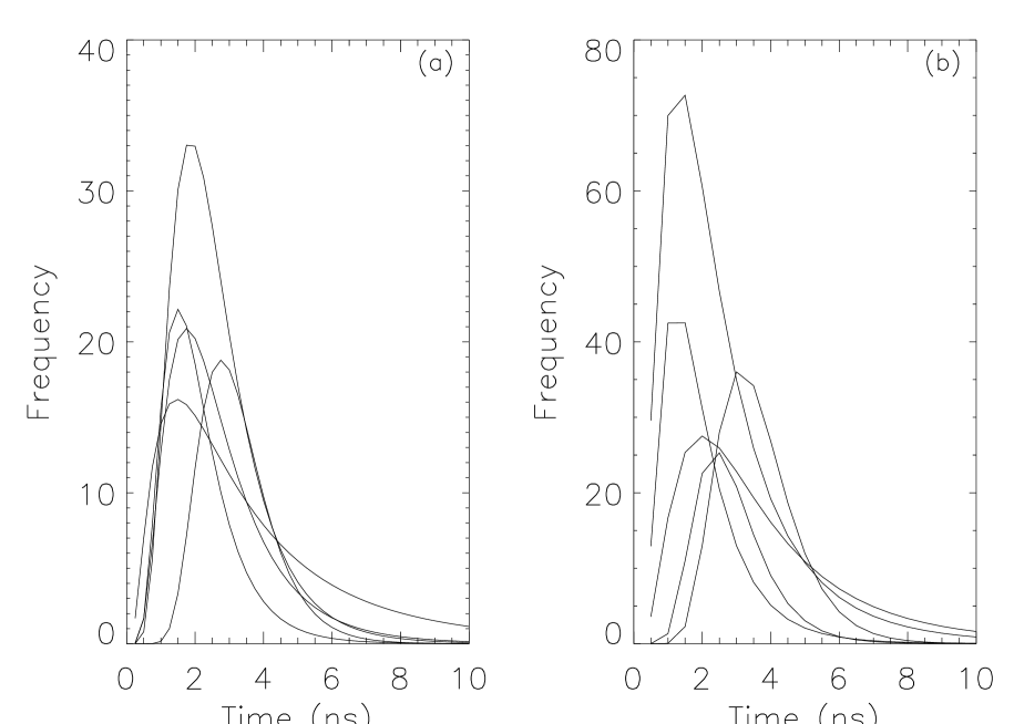
Figure 4: Lognormal fits to arrival time distributions of Čerenkov photons generated by 5 showers of (a) 500 GeV $\gamma-$rays and (b) 1 TeV protons as incident on a detector in the pre-hump region.

The sharp precursor pulse seen prominently in the case of Fe primary (pre- hump region) is presumably due to Čerenkov light produced by muons. It has been noted that these photons are generated at low altitudes ($1-3~{}kms$) with a very small spread in production height suggesting that they are produced by very few muons. The time separations between the $\mu$ and $e$ generated pulses and the pulse shape of the former are comparable with that reported by Cabot $et~{}al.$[18] as well as Roberts et al.[19].

Fig. 4 shows similar fits to Čerenkov pulses in a detector in the pre-hump region from a set of showers generated by (a) 500 GeV $\gamma-$rays and (b) 1 TeV protons. The diversity in the pulse shapes seen here demonstrate the effect of fluctuations in photon number as well as pulse shape parameters.

5 Behaviour of Pulse shape parameters

5.1 Core distance dependence

For each shower, the pulse profile from each detector was fitted with a LDF as mentioned before. For each detector, the arithmetic mean and the variance were calculated from the data set consisting of individual arrival times of detected Čerenkov photons by a detector at a given core distance. The LDF parameters $\mu$ and $\sigma$ are then derived using the mean and RMS from the data, as described in appendix B. Using these derived values of $\mu$ and $\sigma$ as initial guesses, pulse profile, which is suitably binned, is fitted. Using the expressions given in appendix B, pulse shape parameters, which include rise time, decay time and FWHM, are calculated both for derived and fitted LDF parameters. It may be noted that the pulse shape parameters calculated directly from the data (which are sometimes referred to as predicted parameters) are free from systematic errors arising out of data binning.

5.1.1 $\gamma-$ray and proton primaries

Fig. 5a shows the variation of mean rise time (duration for the pulse to reach from 10% to 90% of maximum height), as a function of core distance generated by $\gamma-$ rays of energy 500 GeV. Average is taken over 10 showers. Rise time from the predicted LDF is shown with a continuous line and that from the fitted LDF is shown by diamonds. Shower to shower fluctuations for predicted and fitted rise time are shown in fig. 5b. expressed in terms of RMS/mean. There is a good agreement between the predicted and fitted rise times at all core distances, indicating that in practice there is no need to fit the pulse profiles explicitly.

Figure 5: $(a)$ Radial variation of mean rise time of a Čerenkov pulse, generated by $\gamma-$ ray primaries of energy 500 GeV and $(c)$ 1 TeV protons incident vertically at the top of the atmosphere. Average is taken over 10 showers for each detector. Rise time from the predicted LDF is shown as a continuous line, whereas that from the fitted LDF is shown with diamonds. $(b)$ Variation of shower to shower fluctuations of rise time in terms of RMS/mean as a function of core distance for predicted (continuous line) and fitted distribution functions (broken line) for $\gamma-$ ray primaries and $(d)$ for proton primaries.

Fig. 5c shows core distance dependence of rise time for proton primaries of energy 1 TeV. Again there seems to be a good agreement between predicted and fitted rise times. While the rise times per se are not species dependent, shower to shower fluctuations in proton showers, as shown in fig. 5d, are larger compared to the corresponding fluctuations for $\gamma-$ rays by about a factor of 1.5 - 2.0.

Figure 6: $(a)$ Radial variation of mean decay time of a Čerenkov pulse, generated by $\gamma-$ ray primaries of energy 500 GeV and $(c)$ 1 TeV protons incident vertically on the top of atmosphere. Average is taken over 10 showers for each detector. Decay time from the predicted LDF is shown as a continuous line, whereas that from the fitted LDF is shown with diamonds. $(b)$ Variation of shower to shower fluctuations of decay time in terms of RMS/mean as a function of core distance for predicted (continuous line) and fitted distribution function (broken line) for $\gamma-$ray primaries and $(d)$ for proton primaries.

Variation of decay time (defined as the time duration during which pulse falls from 90% to 10% of maximum height) with core distance for $\gamma-$ ray and proton primaries is shown in figs. 6a and 6c respectively. Decay times from proton primaries are marginally longer than those from $\gamma-$ray primaries. Also shown in the same figure (6b and 6d respectively) are the relative shower to shower fluctuations in decay times. Once again the proton primaries exhibit larger fluctuations compared to those from $\gamma-$ray primaries. In both the cases agreement between the predicted and fitted decay times is poorer at larger core distances mainly because of the paucity of photons and uncertainties due to binning. Shower to shower fluctuations too contribute to this discrepancy.

Figure 7: $(a)$ Radial variation of mean FWHM of a Čerenkov pulse, generated by $\gamma-$ ray primaries of energy 500 GeV and $(c)$ 1 TeV protons incident vertically at the top of atmosphere. Average is taken over 10 showers for each detector. FWHM from the predicted LDF is shown as a continuous line, whereas that from the fitted LDF is shown with diamonds. $(b)$ Variation of shower to shower fluctuations of FWHM in terms of RMS/mean as a function of core distance for predicted (continuous line) and fitted distribution function (broken line) for $\gamma-$ray primaries and $(d)$ proton primaries.

Radial dependence of FWHM for $\gamma-$ ray and proton primaries is shown in figs. 7a and 7c, respectively. A general agreement is seen between the predicted and fitted FWHM. Also shown in the same figure (7b & 7d respectively) are the relative shower to shower fluctuations in FWHM for $\gamma-$ray and proton primaries. Once again the relative fluctuations are about a factor of 2 higher in the case of latter species. For all the pulse shape parameters discussed above, $\gamma-$ ray showers show a better agreement between the fit and prediction compared to protons because of reasons mentioned before.

The radial variations of the relative errors on the pulse shape parameters as shown in figs. 5b, 5d, 6b, 6d, 7b & 7d are not greatly influenced by the number of showers used. They have, however, rather large errors of 47%, 26% and 30% respectively for rise time, decay time and FWHM arising primarily from the small number of showers used here. The peaks seen in the case of $\gamma-$ray primaries are more a result of the mean values showing a minimum at the position of the hump.

5.1.2 Fe primaries

Figure 8: Radial variation of mean $(a)$ rise time, $(c)$ decay time and $(e)$ FWHM of a Čerenkov pulse, generated by primary Fe nuclei of energy 10 TeV. Average is taken over 10 showers for each detector. Rise time from the predicted LDF is shown as a continuous line, whereas that from the fitted LDF is shown with diamonds. Variation of shower to shower fluctuations of $(b)$ rise time, $(d)$ decay time and $(f)$ FWHM in terms of RMS/mean as a function of core distance for predicted (continuous line) and fitted distribution function (broken line).

Figure 8a, 8c & 8e show the radial variation of rise time, decay time and FWHM respectively for a primary iron nucleus of energy 10 TeV incident vertically at the top of the atmosphere. It can be seen that the predicted rise time alone is consistently smaller than that obtained by fitting a LDF while decay time and FWHM show a good agreement between the two. It was noticed that in the case of Fe primaries the pulse profile shows a rather long tail due to a few Čerenkov photons arriving at large delays. The LDF is inadequate to fit these few isolated stragglers and hence the fitted parameters are not affected. The derived parameters, on the other hand, are affected by these delayed photons. This is also reflected in the fact that the LDF generated by the parameters derived from the data show a poor fit resulting in large $\chi^{2}$ value while the fitted LDF shows a $\chi^{2}$ around 1.0. In short, for Fe primaries, the derived values of decay time and FWHM do represent the true value while the rise time does not.

Similarly, figures 8b, 8d & 8f show the relative shower to shower fluctuations of rise time, decay time and FWHM respectively for Fe primaries. As for proton primaries the relative fluctuations are generally larger than those for $\gamma-$ray primaries and are almost independent of core distance. The relative fluctuations computed for derived & fitted parameters are generally in agreement with each other in all the three cases.

5.2 Primary species dependence

The sensitivity of the pulse shape parameters to the primary species can be judged by a comparison of their radial variation for $\gamma-$rays, proton and Fe primaries as shown in figures 5-8. It may be seen that the proton & Fe primaries exhibit larger shower to shower fluctuations as expected. However the magnitude of pulse rise time shows no significant difference for the two types of primaries except that the hadronic primaries show a monotonic increase with core distance. On the other hand pulse fall time and width show more perceptible differences. The possibility of using these parameters for improving the $\gamma-$ray signal strength will be dealt in a forthcoming paper.

5.3 Energy dependence of pulse shape parameters

We have generated several showers of $\gamma-$ rays, with primary energies in the range 0.5-10 TeV, following a powerlaw distribution with index -2.65. Proton showers were also generated following the same power law index, in the energy range 0.5-20 TeV. For each shower, mean pulse shape parameters were derived as described above and averaged over all the detectors. Fig. 9 shows the variation of different pulse shape parameters with primary energy. The sample consists of 34 showers of $\gamma-$ rays and 70 showers of protons. Also shown in the figure are the mean pulse shape parameters, averaged over a number of monoenergetic showers of $\gamma-$ rays and protons. For $\gamma-$ rays of energies 250 GeV, 500 GeV, 1 TeV and 3.5 TeV as well as for protons of energies 500 GeV, 1 TeV, 2 TeV and 5 TeV, mean was calculated over 10, 10, 9 and 4 showers respectively. At lower energies there seems to be rather large fluctuations which are presumably due to the smaller number of Čerenkov photons at lower primary energies. Supported by points derived from monoenergetic showers there seems to be a weak linear correlation between the shape parameters and primary energy.

Figure 9: Variation of average $(a)$ rise time, $(b)$ decay time and $(c)$ FWHM of Čerenkov pulse with primary energy for $\gamma-$ rays. Similar variation for proton showers is shown in $(d)$, $(e)$ and $(f)$, respectively. Pulse shape parameters averaged over all the detectors for each shower are shown by hollow diamonds. For $\gamma-$ rays of energy 250 GeV, 500 GeV, 1 TeV and 3.5 TeV and for protons of energy 500 GeV, 1 TeV, 2 TeV and 5 TeV, mean pulse shape parameters averaged over a number of showers are shown with filled diamonds along with RMS error. For monoenergetic showers variation of pulse shape parameters with energy are fitted with a relation $AE^{-\alpha}$, where E is energy of the primary species. Values of A and $\alpha$ are indicated in the figure for each parameter.

5.4 Altitude dependence

Figure 10: Radial variation of average $(a)$rise time, $(b)$ decay time and $(c)$ FWHM of a Čerenkov pulse as observed at sea level and the same ($d$, $e$ and $f$ respectively) at an observation level of 2.2 km above mean sea level from 500 GeV $\gamma-$ rays incident vertically at the top of atmosphere. Pulse shape parameters derived from the LDF are shown as a continuous line while fitted values are shown as diamonds.

Figure 11: Radial variation of average $(a)$rise time, $(b)$ decay time and $(c)$ FWHM of a Čerenkov pulse as observed at sea level and the same ($d$, $e$ and $f$ respectively) at an observation level of 2.2 km above mean sea level from 1 TeV protons incident vertically at the top of atmosphere. Pulse shape parameters derived from the LDF are shown as a continuous line while fitted values are shown as diamonds.

Radial variation of all the three pulse shape parameters were studied at two other observation levels both for $\gamma-$ray and proton primaries. Figure 10 shows the variation of rise time, decay time and FWHM of the Čerenkov pulses as measured at various core distances for $\gamma-$rays of energy 500 GeV incident vertically at the top of atmosphere. The panels labeled a, b & $c$ correspond to sea level while those labeled d, e & $f$ correspond to an observation level of 2.2 km. Similarly, Figure 11 shows the corresponding behavior for proton primaries of energy 1 TeV.

It can be readily noticed that for $\gamma-$ray primaries there is practically no change in the radial variation in the three parameters until the hump region. However beyond the hump region some parameters seem to vary faster at higher altitudes. The range of rise time, decay time and FWHM at the three different observation levels are listed in table 5. It can be seen from the table that both for $\gamma-$ray and proton primaries, the maximum values of all the three pulse shape parameters viz. rise time, decay time & FWHM at large core distances show a systematic increase with increase in observation level showing their possible sensitivity to altitude. However assuming that a diverging Čerenkov cone is being intercepted at different observation levels, one would expect such an increase at higher altitudes due to simple geometric effects. Let us see if this indeed is the reason for this apparent increase.

Since the linear increase in the parameter begins from the position of the hump, it is obvious that the hump position plays an important role here. Therefore we estimated the core distance of the hump for a 500 GeV $\gamma-$ray primary to be 143 $m$, 130 $m$ and 116 $m$ respectively at three altitudes sea-level, 1070 $m$ and 2200 $m$ above mean sea-level. These values are consistent with earlier estimates by Rao & Sinha [20]. It may be seen that at equal radial distances, measured from the hump position at a given level, the shape parameters have similar values at each altitude of observation. Thus, the shape parameters do not have intrinsic sensitivity to the observation altitude. The same seems to hold good for proton primaries as well even though their lateral distribution does not exhibit any prominent hump [14].

Table 5: Range of radial variation of rise time, decay time and the FWHM of the Čerenkov pulse profile at various observation levels.

Species	Energy	Observation
	GeV	Level ((km)
		Above mean	Rise Time	Decay Time	FWHM
		sea level)	ns	ns	ns
$\gamma-$ rays	500	0.0	0.35 - 1.5	2 - 16	1 - 6.5
		1.0	0.35 - 1.5	2 - 17	1 - 7
		2.2	0.3 - 2.2	2 - 24	1 - 10
Protons	1000	0.0	0.3 - 1.35	4 - 21	2 - 6.5
		1.0	0.35 - 1.8	5 - 23	2 - 8.5
		2.2	0.3 - 1.9	4 - 29	2 - 12

5.5 Incident angle dependence

Figure 12: Radial variation of average $(a)$ rise time, $(b)$ decay time and $(c)$ FWHM of a Čerenkov pulse as observed at Pachmarhi from 500 GeV $\gamma-$rays and the same quantities ($d$, $e$ and $f$ respectively) from 1 TeV protons incident at an angle of $30^{\circ}$ with respect to vertical at the top of atmosphere. Pulse shape parameters derived from the LDF is shown as a continuous line while the fitted values are shown as diamonds.

Figures 12a, 12b & 12c show the radial variation of rise time, decay time and the pulse width for 500 GeV $\gamma-$ray primaries incident at an angle of 30^∘ to the vertical at the top of atmosphere at Pachmarhi. Similarly figures $12d,~{}12e~{}\&~{}12f$ show the corresponding variations for primary protons of energy 1 TeV.

There are some noticeable differences between the Čerenkov pulse shape characteristics of inclined showers compared to those of vertical showers for both the types of primaries. Inclined $\gamma-$ray showers exhibit a larger change in the pulse shape parameters in the core to hump region even though the variation is comparable to the shower to shower fluctuations as in the case of vertical showers. Radial variation of relative shower to shower fluctuations on the other hand seems to be more uniform and reduced in magnitude at larger incident angles as shown in table 6. This could be a result of additional Coulomb scattering of electrons due to increased path lengths for inclined showers. The hump also moves away from the core by a $sec(\theta)$ factor.

Similarly, in the case of inclined proton showers the pulse shape parameters have larger values near the core and remain more uniform as a function of core distance compared to that for vertical showers. Both for $\gamma-$ray and proton primaries which do not have significant muon content at the energies studied here the rise time distribution broadens slightly with increasing zenith angle as expected from the increased distance from the shower maximum [19].

Table 6: Range of radial variations of relative shower to shower fluctuations in rise time, decay time and the FWHM of the Čerenkov pulse profile for vertical and inclined showers.

Species	Energy	Incident	Rise Time	Decay Time	FWHM
	GeV	Angle (∘)
$\gamma-$ rays	500	0.0	0.35 - 0.75	0.25 - 0.4	0.25 - 0.5
		30.0	0.24 - 0.4	0.17 -0.25	0.15 - 0.24
Protons	1000	0.0	0.6 - 0.85	0.45 - 0.7	0.45 - 0.8
		30.0	0.5 - 0.8	0.25 - 0.55	0.15 - 0.6

6 Discussions

6.1 The Spherical Shower front

Figure 13: A plot of the Čerenkov photon arrival times as a function of production height, at three different core distance ranges: pre-hump, hump & post hump regions. The primary is a gamma ray of energy 550 GeV incident vertically on the top of the atmosphere.

Figure 14: A plot of the Čerenkov photon arrival angle as a function of production height, at three different core distance ranges: pre-hump, hump & post hump regions. The primary is a gamma ray of energy 550 GeV incident vertically on the top of the atmosphere.

Qualitatively, the temporal radial profiles are largely independent of the species. It can be seen from figures 2 & 3 that the arrival time delay increases at larger core distances giving rise to longer tails in the post hump region. How do we understand this? The increase in the average delay as a function of core distance reflects the fact that moving to the outer regions of the shower, the average energy of the electrons, the progenitors of the Čerenkov photons, decreases and therefore the deviations from a straight line trajectory become more important. Figure 13 shows a plot of the photon arrival time as a function of their production height, at various core distance ranges. It can be seen that at near core distances the Čerenkov photon arrival times are almost directly proportional to their production heights and are produced lower down in the atmosphere. However around the hump region, the light reaches the observation level first from higher altitudes and a majority of the light can be seen to originate higher up in the atmosphere. At larger core distances however a bulk of the photons are produced lower down in the atmosphere consistent with the simplified picture of Hillas [21]. A similar plot of arrival angles as shown in figure 14 shows that the photons produced at lower heights arrive at larger incident angles resulting mainly from multiple Coulomb scattering. Also the photons at hump and the region beyond have large arrival angles thus leading to the increased arrival times as seen. Hence beyond a core distance of $\sim$ 50 m, the light arrival time directly relates to their altitude of origin.

It has been shown by Hammond et al. [4] that for a vertical shower the time taken by a photon emitted at a height R to reach a core distance r follows a quadratic function which is approximated to a function shown in equation 1 for a fixed height R from the observation level. Hence the spherical shape of the Čerenkov light front is purely a geometric effect, accentuated by the fact that a bulk of the Čerenkov light is produced at the shower maximum. Therefore the shape of shower front is primarily determined by the height of shower maximum and is practically independent of species as well as altitude as confirmed by the present results as well as by those of Protheroe et al. [22].

6.2 Pulse shape parameters

Both lognormal and $\Gamma-$function fits to the arrival time delay distributions of shower secondaries have been tried by others as well. Fitting a lognormal distribution to Čerenkov pulse profiles is done here for the first time. Battistoni et al.[11] fitted these functions to the delay distributions of secondary $\gamma$’s and ${\mathit{e}^{\pm}}$ from primary $\gamma-$rays and protons. They conclude that lognormal distribution fits the data better than the gamma function mainly because of the long tails at large delays ($\sim$ 200 ns). At larger delays even the lognormal function does not fit the tail adequately and hence they use additional terms in the Graham-Charlier expansion consisting of a series of derivatives of the standard lognormal function. Rodríguez-Frías et al.[23] on the other hand use $\Gamma$-function to fit the average Čerenkov pulses generated by primary $\gamma-$rays and hadrons of energy $>$ 1 TeV. They find that the function gives a good fit atleast for photon delays $<~{}30~{}ns$, even though no mention is made of the quality of fit obtained by them.

In the present work we consider only delays $<~{}30~{}ns$. Hence we find the quality of fit to the delay distributions to the two functions is comparable even though lognormal function, which has a slight edge, is used for further studies based on the fit. As shown in the Appendix B one can derive the observable pulse shape parameters like the rise time, decay time and the pulse width from mean pulse arrival time and the arrival time jitter which are far more easier to measure.

Table 7: Summary of the Čerenkov photon arrival angle distribution at the observation level for three different primary energies. The primary is a $\gamma-$ray incident vertically at the top of the atmosphere. The statistical parameters listed below are derived from all the detected photons over all core distances in the range $0~{}-~{}280~{}m$. The mean is computed over 50, 20 and 10 showers respectively for 100, 500 & 1000 GeV primaries.

Energy	Mean	RMS	Skewness
GeV
100	0.87	0.47	1.06
500	1.73	0.69	1.39
1000	1.91	0.75	1.46

It has been argued in the past that the near sphericity of the Čerenkov light fronts requires that the pulse shape parameters should have a quadratic dependence on core distance [24]. Our results for photonic as well as hadronic primaries are consistent with this hypothesis for core distances beyond $\sim 150~{}m$. A steeper dependence seen at higher observation levels could be the result of shorter distance between the shower maximum and the observation level. Average pulse shape parameters exhibit a minimum at a core distance of around $150~{}m$, which is the position of the hump for $\gamma-$ray primaries, consistent with earlier studies [21]. It is expected since the photons arriving here are produced mainly by energetic electrons in the cascade [20,21]. However it may be noted that for a given primary the observed variation at short core distances ($\leq$ 150 m) is comparable to the shower to shower fluctuations of these parameters.

It may be noted that the main reason for the asymmetric pulse shapes discussed here is due to the large acceptance angles (unrestricted) of incident photons. After limiting the detector opening angle to $\pm 1^{\circ}$ with respect to the shower axis, it has been verified that the Čerenkov pulse profiles become narrower and more symmetric. This demonstrates that the long tails are contributed by photons incident at large angles. Cabot et al.[18] generate the Čerenkov pulse profile for vertically incident protons of energy 10 TeV which is in agreement with the present results for lower energy protons as shown in figure 3. It can be seen from their figures 2 & 3 that by applying an angular cut of $\pm 20~{}mrad$ for the incident Čerenkov photons, the pulse profile becomes narrower and symmetric while a bulk of the tail at large delays vanishes. For the same reason the average Čerenkov pulse profiles generated by Roberts et al. [19] using monte carlo technique, are comparatively narrower and less skewed. The main reason for this is that the opening angle of the Čerenkov telescopes for which simulations are carried out by them is around $1.3^{\circ}$ FWHM. In addition, these simulations are carried out for higher energy (50 TeV) primaries incident at large zenith angles $(35^{\circ}~{}\&~{}65^{\circ})$. More recently, the pulse shape generated for a limited field of view of the HEGRA imaging telescope by Heß  et al. [25] also is narrower and symmetric, once again supporting the above argument.

Pulse shape parameters, which represent the cascade development characteristics, are not expected to be sensitive to primary energy since the development of showers in the atmosphere is initiated by the first interaction point which, in turn, is determined by the interaction length (for a given primary species). From the present simulations we find that for for both types of primaries, the weak dependence of rise time, fall time and FWHM on the primary energy can be parameterized as a power law in energy as shown in figure 9. For $\gamma-$ray primaries there is a weak but definite energy dependence showing that each of the three pulse shape parameters increase with primary energy. This is mainly because the photon arrival angle distribution exhibits larger fluctuations and becomes more skewed at higher primary energies as shown in table 7. For proton primaries, on the other hand, the dependence is uncertain because of large errors in the fitted parameters. Considering the errors on the slopes, our results are consistent with the expected energy independence. However because of the logarithmic increase in the interaction cross-section with energy, a mild increase with primary energy is expected. Considering the large errors on the fitted parameters and the limited energy range considered here, we can conclude that these fits are consistent with the simulation results at higher primary energies which show that the pulse shape parameters do increase with energy [4,23].

7 Conclusions

The radius of curvature of the Čerenkov shower front shows a strong correlation with the height of shower maximum and is practically independent of other observational parameters. Čerenkov light pulse shape measurements now play an important role in the analysis of atmospheric Čerenkov data and as independent measures within the shower, complement photon density measurements. Within the range of delays considered here lognormal distribution function represents the pulse shapes fairly accurately at all core distances up to a maximum of $280~{}m$. Among the three pulse shape parameters considered here fall time seems to be most sensitive to the primary species.

We would like to acknowledge the fruitful discussions with Profs. K. Sivaprasad, B. S. Acharya and P. R. Vishwanath during the present work.

Appendix A: $\Gamma-$ function

A $\Gamma-$ function distribution, f(x) is defined as [17]:

$$f(X)={{a\left[aX\right]^{b-1}exp(-aX)}\over{\Gamma(b)}}$$ (4)

where $X$, $a$ and $b$ are real positive numbers.

The expectation value of X is given by:

$$E(X)={{b}\over{a}}$$ (5)

and the variance of $X$ is given by:

$$V(X)={{b}\over{a^{2}}}$$ (6)

Maximum functional value is obtained by solving the equation:

$${{df}\over{dX}}=0$$ (7)

The solution for which is

$$X_{max}={{b-1}\over{a}}$$ (8)

$a$ and $b$ in the $\Gamma-$ function can be expressed in terms of peak position $X_{max}$ and the mean value $<X>$ using the equations given above. Hence $\Gamma-$ function could be defined in terms of the newly chosen variables as:

$$f(X)=C\times X^{\left({X_{m}ax}\over{<X>-X_{max}}\right)}exp{\left(-{{X}\over{<X>-X_{max}}}\right)}$$ (9)

where

$$C={{a^{b}}\over{\Gamma(b)}}$$

However, in order to use this expression it is necessary to know the position of the pulse peak. Hence it is necessary to suitably bin the arrival times at the detector and generate a pulse profile. The estimate of the pulse peak position can therefore be bin dependent. We have tried to avoid this dependence on binning, by obtaining the initial estimates of pulse parameters after expressing $a$ and $b$ in terms of expectation value [$E(X)$] and variance [$V(X)$]. These are arithmetic mean and variance of the data, derived using equations given above. Hence

$$a={{E(X)}\over{V(X)}}$$ (10)

and

$$b=a\times E(X)$$ (11)

These values of $a$ and $b$ are used as initial estimates while fitting pulse profile to a Gamma distribution function. However one cannot easily derive the pulse shape parameters like rise & fall times and full width of the pulse, using $a$ and $b$.

Appendix B: Lognormal distribution

A positive variate $x$ $(0<x<\infty)$ follows a lognormal distribution when its logarithm $y=logx$ is normally distributed with mean $\mu$ and variance $\sigma^{2}$. Distribution function is given by [26]:

$$P(x)={{1}\over{x\sigma\sqrt{2\pi}}}exp{\left[-{{1}\over{2\sigma^{2}}}\left(logx-\mu\right)^{2}\right]}$$ (12)

The $j$th moment of the distribution about the origin is given by:

$$\lambda^{\prime}_{j}=exp\left(j\mu+{{1}\over{2}}j^{2}\sigma^{2}\right)$$ (13)

Hence the mean $\alpha$ and variance $\beta^{2}$ are given by

$$\alpha=exp\left(\mu+{{1}\over{2}}\sigma^{2}\right)$$ (14)

and

$$\beta^{2}=exp(2\mu+\sigma^{2})\left(exp(\sigma^{2})-1\right)=\alpha^{2}\eta^{2}$$ (15)

where $\eta^{2}=exp(\sigma^{2})-1$

For a given data set arithmetic mean $\alpha$ and variance $\beta^{2}$ can be estimated and using the equations given above. $\mu$ and $\sigma^{2}$ can be calculated after inverting the equations 3 & 4 as:

$$\mu={log{\alpha}}-{{1}\over{2}}{\sigma^{2}}$$ (16)

$$\sigma^{2}=log\left(1+{{\beta^{2}}\over{\alpha^{2}}}\right)$$ (17)

and then the corresponding lognormal distribution can be generated. The values of $\mu$ and $\sigma^{2}$ so obtained are used as initial estimate while fitting lognormal distribution to pulse profile.

Median and mode of the distribution are given by $exp(\mu)$ and $exp(\mu-\sigma^{2})$, respectively.

Value of the distribution function at the mode is given by

$$P_{max}={{1}\over{\sigma\sqrt{2\pi}}}exp\left[{{\sigma^{2}}\over{2}}-\mu\right]$$ (18)

FWHM of the distribution, i.e, the width where value of the distribution function is $P_{max}/2$, can be obtained solving equation 1, after substituting for $P_{max}$ from equation 7. It is given by,

$$w=exp\left(\mu-\sigma^{2}\right)\left[exp\left(\sqrt{-2\sigma^{2}log(0.5)}\right)-exp\left(-\sqrt{-2\sigma^{2}log(0.5)}\right)\right]$$ (19)

Rise time and decay time can be calculated using a similar procedure. They are given by following expressions:

$$\tau_{r}=exp\left(\mu-\sigma^{2}\right)\left[exp\left(-\sqrt{-2\sigma^{2}log(0.9)}\right)-exp\left(-\sqrt{-2\sigma^{2}log(0.1)}\right)\right]$$ (20)

$$\tau_{d}=exp\left(\mu-\sigma^{2}\right)\left[exp\left(\sqrt{-2\sigma^{2}log(0.1)}\right)-exp\left(\sqrt{-2\sigma^{2}log(0.9)}\right)\right]$$ (21)

References

- [1] Cronin, J. W., Gibbs, K. G. and Weekes, T. C., 1993, Ann. Rev. Nucl. Part. Sci., 43, 883.
- [2] Fegan, D. J., 1997, J. Phys. G: Nucl. Particle Phys., 23,1013.
- [3] Schubnell, M. S., et al., 1996, Astrophys. J., 460, 644.
- [4] Hammond et al., 1978, Nuovo Cim., 1C, 315.
- [5] Knapp, J. and Heck, D., 1998, EAS Simulation with CORSIKA, V5.60: A user’s Guide.
- [6] Nelson, W. R., 1985, The EGS4 Code System, SLAC Report 265.
- [7] US Standard Atmosphere, 1962, (US Govt. Printing Office, Washington).
- [8] Bhat, P. N., 1998, “High Energy Astronomy & Astrophysics” , Proc. of the Int. Colloquium to commemorate the Golden Jubilee year of Tata Institute of Fundamental Research, Ed: P. C. Agrawal and P. R. Vishwanath, University Press, 370
- [9] Ford, R. L. and Nelson, W. R., 1978, SLAC Report # 210.
- [10] Aglietta, M. et al., 1993, Nucl. Inst. and Meth., A336, 310.
- [11] Battistoni, G., Ferrari, A., Carboni, M. and Patera, V., 1998, Astropart. Phys., 9, 277.
- [12] Acharya, B. S. et al., 1993, J. Phys. G:Nucl. Part., 19, 1053.
- [13] Krawczynski, H. et al., 1996, Nucl. Instr. and Meth., A 383, 431.
- [14] Chitnis, V. R. and Bhat, P. N., 1998, Astropart. Phys. 9, 45.
- [15] Efimov, N. N., et al., 1973, III Int. Cosmic Ray Conf. (Denver, Col.), 4, 2378.
- [16] Fomin, Yu. A. and Khristiansen, G. B., 1971, Soviet J. Nucl. Phys., 14, 360.
- [17] Eadie, W. T., Drijard, D., James, F. E., Roos, M. and Sadoulet, B., 1971, “Statistical Methods in Experimental Physics”, North Holland Pub. Co., Amsterdam, p 80.
- [18] Cabot, H., et al., 1998, Astropart. Phys., 9, 269.
- [19] Roberts, M. D., et al., 1998, J. Phys. G: Nucl. Particle Phys., 24, 255.
- [20] Rao, M. V. S. and Sinha, S., 1988, J. Phys. G:Nucl. Part., 14, 811
- [21] Hillas, A. M., 1982, J. Phys. G: Nucl. Part. Phys., 8, 1475.
- [22] Protheroe, R. J., Smith, G. J. and Turver, K. E., 1975, Proc. XIV Int. Cosmic Ray Conf., Munich, 8, 3008.
- [23] Rodríguez-Frías, M. D., del Peral, L. and Medina, J., 1995 Nucl. Instr. and Meth., A 355, 632.
- [24] Orford, K. J. and Turver, K. E., 1976, Nature, 264, 727.
- [25] Heß, M., et al., 1998, Astro-ph/9812341.
- [26] Aitchison, J., and Brown, J. A. C., 1957, “The Lognormal Distribution”, The University Press, Cambridge, p8.