Implications of H$\alpha$ Observations for Studies of the Cosmic Microwave Background

Abstract

We summarize the relationship between the free-free emission foreground and Galactic H$\alpha$ emission. H$\alpha$ observations covering nearly the entire celestial sphere are described. These data provide a template to isolate and/or remove the effect of Galactic free-free emission from observations of the cosmic microwave background. Spectroscopy and imaging provide two complementary methods for measuring the H$\alpha$ emission. Spectroscopy is favored for its velocity resolution and imaging is favored for its angular resolution. With templates of the three dominant foregrounds, namely synchrotron, thermal dust, and free-free emissions, it may be possible to quantify the location and the brightness of another foreground such as that from rotating dust grains.

Astronomy Department, University of Illinois at Urbana-Champaign, Urbana, IL 61801

Physics & Astronomy Dept., Swarthmore College, Swarthmore, PA, 19081-1397

Las Cumbres Observatory, Los Gatos, CA 95033

IPAC/Caltech, Pasadena, CA 91125

1. Introduction

Cosmologists interested in the anisotropy of the Cosmic Microwave Background (CMB) must observe from within the Milky Way. Thus, they must measure and subtract foreground emissions from the Milky Way. Three important components of foreground emission have long been recognized: 1) thermal emission from dust, 2) synchrotron emission from relativistic electrons accelerated by magnetic fields, and 3) bremsstrahlung (“braking” radiation or “free-free” emission) from free electrons accelerated by interactions with ions in a plasma. A fourth component associated with rotating dust has also been proposed recently (Draine & Lazarian 1998).

This review addresses the Galactic free-free emission and its tracer H$\alpha$ light. It treats the warm ionized medium (WIM) as an unavoidable foreground that must be accounted for in the interpretation of microwave observations of the CMB. That is, it treats the WIM phenomenologically and does not discuss why the WIM is the way it is.

From that viewpoint, the problem with free-free radiation is two-fold. First, whereas at low frequencies ($\nu\mathrel{\hbox{\hbox to0.0pt{\hbox{\lower 4.0pt\hbox{$\sim$}}\hss}\hbox{$<$}}}20$ GHz) synchrotron emission dominates, and at high frequencies ($\nu\mathrel{\hbox{\hbox to0.0pt{\hbox{\lower 4.0pt\hbox{$\sim$}}\hss}\hbox{$>$}}}100$ GHz) dust emission dominates, in between ($\nu\approx 30$ GHz) free-free emission is as bright or brighter than the other two. That is, we have leverage on synchrotron and dust, but not free-free. We need a tracer of free-free to solve the first problem (lack of leverage), and that tracer is H$\alpha$ light. The second problem has been – until very recently – the lack of all-sky observations of H$\alpha$. The H$\alpha$ data that solve the second problem now exist and are being calibrated and rendered into a template suitable for decontaminating the free-free foreground.

This review is organized as follows. The next section is a short historical vignette to give context to modern efforts. Section 3 lists other reviews similar to this one. Section 4 relates H$\alpha$ and free-free emissions in Equation 4, Figure 1, and Table 1. Section 5 describes and compares the two principle techniques for observing H$\alpha$, Fabry-Perot spectroscopy and narrowband imaging. Typical results are shown and inherent challenges are noted. Section 6 addresses the association of dust and ionized gas. Finally, Section 7 concludes with a short summary of how the H$\alpha$ data will be used in practice to decontaminate the microwave observations.

Figure 1.: Foreground contaminants of the CMB are plotted along with the five bands of the MAP satellite. At low frequencies ($\nu\mathrel{\hbox{\hbox to0.0pt{\hbox{\lower 4.0pt\hbox{$\sim$}}\hss}\hbox{$<$}}}20$ GHz) synchrotron emission dominates, while at high frequencies ($\nu\mathrel{\hbox{\hbox to0.0pt{\hbox{\lower 4.0pt\hbox{$\sim$}}\hss}\hbox{$>$}}}100$ GHz) dust emission dominates, and in between free-free emission is as bright or brighter than the other two. For the synchrotron, thermal dust, and free-free bands, the upper line corresponds to $|b|\approx 15$^∘, and the lower line corresponds to $|b|\approx 65$^∘. The bands are reproduced from Bennett et al (1992). The Bennett et al. model has more free-free emission than models based upon H$\alpha$ observations (cf. Equations 2 and 4). The sloped, dashed line illustrates the free-free emission corresponding to an H$\alpha$ surface brightness of 1 Rayleigh. The curved line illustrates the emission from rotating dust predicted by Draine & Lazarian (1998) for the North Celestial Pole region studied by Leitch et al. (1997). The five frequencies of the MAP satellite are 22, 30, 40, 60, and 90 GHz.

2. Yesteryear

It is interesting to compare today’s remote– and robotic–observing in Section 5 with heroic efforts from a century ago. E. E. Barnard claims to have seen with his own eye that which we now call “interstellar cirrus.” He photographed filaments of dust in the Taurus region, far from the bright reflection nebulosity of the Pleiades, and remarked “it was the knowledge of their existence by visual observations alone that led me to make the photographs” (Barnard 1896). For one such photograph, a 10-hour exposure, Barnard kept the plate in the camera for over fifty hours. Unsatisfied with the duration of the exposure at the end of the first night, he waited for a second night, but it was cloudy, so he resumed the exposure the third night, after re-aligning the guide star to its original location. Barnard’s photographs of the filaments streaming away from the Pleiades look astonishingly like the 100 $\mu$m image of IRAS (cf. plate 10 of Barnard (1900) or plate 8 of Barnard (1928), which is in Arny (1989), to the IRAS image of Souras (1989)). Those same filaments absorb background H$\alpha$ (Figure 5), which is unusual at moderate Galactic latitudes and contrary to the positive correlation between H$\alpha$ and dust discussed in Section 6.

The H$\alpha$ line is included in the pass band for the red plates of the National Geographic Society/Palomar Observatory Sky Survey (POSS 1), and these show very bright emission nebulae. Because they lack the sensitivity to detect the low-surface-brightness WIM, the POSS plates can give a false impression that ionized gas exists only in Stromgren spheres, when in fact most (90%) of the Milky Way’s ionized gas is outside individual Stromgren spheres around OB stars (Reynolds 1993). The next generation plates (POSS 2) are sensitive to emission of $\sim 25$ R, or $\sim$4 times fainter than POSS 1, but for both POSS 1 and POSS 2, it is impossible to identify and quantify the emission specifically from the H$\alpha$ line because the filters are broadband.

Sivan (1974) conducted a photographic survey in search of the WIM, reaching a limiting brightness of 15 R and covering low Galactic latitudes ($|b|\mathrel{\hbox{\hbox to0.0pt{\hbox{\lower 4.0pt\hbox{$\sim$}}\hss}\hbox{$<$}}}$ 20^∘) at a resolution of approximately 10^′. Later, Parker, Gull, and Kirschner (1979), using an image tube camera, produced an atlas of images in four emission lines ([SII],H$\alpha$ +[NII], O[III], H$\beta$) and the blue continuum (4220 Å), which covered low Galactic latitudes ($|b|\mathrel{\hbox{\hbox to0.0pt{\hbox{\lower 4.0pt\hbox{$\sim$}}\hss}\hbox{$<$}}}8$^∘) at an angular resolution of 0.6^′ and sensitivity of 15 R.

3. Other Reviews

In this section I note briefly recent reviews similar to this one. Each of the other reviews describe the physical relationship between the H$\alpha$ and free-free emissions and their implications for observing the CMB. Smoot (1998) reviews the topic as it was in January, 1998. Valls-Gabaud (1998), Bartlett & Amram (1998), and Marcelin et al. (1998) are similar to each other, each with a slightly different emphasis. (Valls-Gabaud, Bartlett, and Amram are co-authors of Marcelin et al.). Valls-Gabaud (1998) is notable for its thorough discussion of the proportionality between the brightness temperature due to free-free $T_{b}^{ff}$ and the surface brightness in H$\alpha$, $I_{\alpha}$.

This review necessarily repeats some of the material in the aforementioned reviews and adds to them the advances of 1998, by the end of which the H$\alpha$ sky had been observed very nearly in its entirety.

4. The free-free/H$\alpha$ ratio

Because there are treatises on the topic of electron-ion interaction (e.g. Mezger & Henderson 1967; Osterbrock 1989, Jackson 1975), and because the papers cited in the previous section summarize the topic, we do not repeat that information here except to note the most basic formulae.

Both free-free and recombination radiation (e.g. H$\alpha$ ) are proportional to the emission measure,

$$EM=\int n_{e}n_{p}dl\approx\int n_{e}^{2}dl.$$ (1)

At moderate Galactic latitudes, the H$\alpha$ emission (which traces the free-free emission) has been modeled as (Reynolds 1992)

$$I_{\alpha}\approx 1.2R/sin|b|$$ (2)

where 1 Rayleigh (R) is defined as

$${\rm 1~{}R=10^{6}/4\pi~{}photons~{}cm^{-2}~{}s^{-1}~{}sr^{-1},}$$ (3)

which for H$\alpha$ corresponds to an emission measure EM = 2.75 cm^-6pc for gas at 10⁴ K (Reynolds 1990), or $2.4\times 10^{-7}$ erg cm^-2 s^-1 sr^-1, or $5.7\times 10^{-18}$ erg cm^-2 s^-1 arcsec^-2. Like the other constituents of the Milky Way, the H$\alpha$  varies considerably across the sky.

The ratio of free-free brightness temperature $T_{b}^{ff}$ to the H$\alpha$ surface brightness $I_{\alpha}$ for Case B recombination is (Valls-Gabaud 1998)

$${{T_{b}^{ff}[mK]}\over{I_{\alpha}[R]}}=10.4\nu^{-2.14}T_{4}^{0.527}10^{0.029/T_{4}}(1+0.08)$$ (4)

where $\nu$ is the observing frequency in GHz, and the last factor (1+0.08) assumes that helium (0.08 by number with respect to hydrogen) is entirely in the form of He⁺, which creates free-free emission like hydrogen, but of course doesn’t emit H$\alpha$ light. This relation is the basis for using H$\alpha$ as a tracer of free-free. It plotted in Figure 1 and is tabulated below.

Table 1.: Free-free to H$\alpha$ ratio

Satellite	Frequency [GHz]	${{T_{b}^{ff}}/{I_{\alpha}}}[~{}{\mu}K~{}R^{-1}~{}]$
COBE	19.2	19.3
	31.5	6.7
	53	2.20
	90	0.71
MAP	22	14.4
	30	7.4
	40	4.0
	60	1.69
	90	0.71

5. Observations

There are two types of H$\alpha$ observations: Fabry-Perot (F-P) spectroscopy and narrowband imaging. Later we describe them separately, but first we discuss issues common to both techniques. Most of the information on the Wisconsin H-Alpha Mapper (WHAM) in this review comes from Tufte (1997) and Haffner (1999). Most of the information on narrowband imaging comes from the experience of the authors.

Both the F-P and the narrowband observations are made under clear, dark skies, when the moon is below the horizon and the sun is more than 18^∘below the horizon.

Both types of observations suffer from the geocoronal emission, which is temporally and spatially variable. The geocorona extends from a base at an altitude of $\sim$500 km to many Earth radii. Lyman-$\alpha$ images taken by spacecraft far above the Earth show a smooth geocorona, decaying exponentially with geocentric distance (Rairden et al. 1986). We know of no such images in Lyman-$\beta$ or Balmer-$\alpha$, but because it is so extended and because it is excited by scattered solar Lyman-$\beta$ light, the geocorona should be rather featureless in H$\alpha$. Measurements of the surface brightness $\Sigma_{geo}$ of the geocorona in H$\alpha$ over many years with instruments like WHAM show variations from 1 to 10 R, primarily dependent on the height at which the telescope’s pointing direction exits the Earth’s shadow (Nossal et al. 1993).

For comparison the Earth-bound, dark-sky surface brightness in continuum ${{d\Sigma_{sky}}\over{d\lambda}}=1.3$ R Å^-1 at H$\alpha$ (Broadfoot & Kendall 1968).

The two techniques use different methods to subtract geocoronal H$\alpha$ emission. The two methods are analogous to frequency switching and position switching. The F-P method is analogous to frequency switching in that a baseline is fit and subtracted as a function of frequency, so the measured brightness at “OFF” frequencies affects the rest of the spectrum. The imaging method is like position switching (a.k.a. chopping) in that a surface is fit and subtracted as a function of position on the sky, so that the H$\alpha$ brightness of the sky is measured relative to other parts of the sky. To be exact, both methods share properties of both frequency and position switching. In the most demanding F-P observations, the beam is switched alternately from a target position to an OFF position; doing so reduces the effects of time-variable telluric emission lines. In the imaging technique, observing alternately through an H$\alpha$ filter and a filter near H$\alpha$ is a form of frequency switching that allows subtraction of continuum but not line emission.

In addition to the geocorona, there are many other challenges to H$\alpha$ observations. There are other airglow lines, especially those from OH in the mesosphere. The H$\alpha$ light from high velocity clouds is within the bandpass of narrowband H$\alpha$ images but is outside the nominal velocity coverage of the WHAM survey. Where they have been observed, high-velocity clouds are weak, $\sim$0.1 R, or $\sim$10% of the H$\alpha$ surface brightness at high latitudes (Tufte, Reynolds, & Haffner 1998). There is continuum emission from the atmosphere, from zodiacal light, from stars and galaxies, individually and collectively. Bright stars saturate small regions of narrowband images and ruin a few WHAM spectra by superposing their Fraunhofer H$\alpha$ absorption lines on the spectra from the WIM.

The Solar H$\alpha$ absorption line must also be present in the night sky spectrum via zodiacal light. We are not aware of a careful analysis of this effect on H$\alpha$ observations of the WIM. A crude estimate is possible. The line’s core is $\sim$1Å wide and is nearly entirely dark ($\sim$20% of the continuum level). At its faintest level, the zodiacal light is $\sim$25% of the dark-sky continuum at H$\alpha$ (1.3 R Å^-1). Thus a $\mathrel{\hbox{\hbox to0.0pt{\hbox{\lower 4.0pt\hbox{$\sim$}}\hss}\hbox{$>$}}}$0.3 R absorption line, $\sim$50 km s^-1 wide, should appear in all F-P spectra. If this estimate is correct, the WHAM data should be sensitive to this effect. If not corrected, the effect will be to underestimate the true brightness of the Galactic H$\alpha$ emission.

Each of the two surveys has completed its “first year” observations, and these data are being calibrated and analyzed. Both the WHAM project and the robotic imaging project at CTIO continue to operate, reobserving some locations. Because WHAM is remotely operated and because the CTIO project is robotically operated, the incremental cost of reobserving is small compared to the original setup costs. Once calibrated, each survey will be published independently (anticipated dates are late-1999 to mid-2000) and then the region of overlap, from declination -30^∘ to +15^∘, or 38% of the entire sky, will be compared in detail.

5.1. Fabry-Perot Spectroscopy

Fabry-Perot H$\alpha$ spectroscopy has been dominated by the work of Ron Reynolds, so much so that the 1-kpc thick layer of the warm ionized medium of the Milky Way is sometimes referred to as the “Reynolds layer.” This has culminated in the WHAM survey (www.astro.wisc.edu/wham/).

The WHAM instrument combines a 0.6-meter telescope and a high-resolution, 15-cm F-P spectrometer. The spectrometer can be pressure-tuned anywhere from 4800Å to 7200Å, but here we discuss only its capabilities at H$\alpha$. Its cryogenically-cooled CCD has high quantum efficiency (78% at H$\alpha$) and low noise (3 e- rms). It is located at Kitt Peak, AZ, and operated remotely from Wisconsin. Fig. 2 shows an example of WHAM’s view of the WIM.

The WHAM survey is a velocity-resolved survey of H$\alpha$ emission over 3/4 of the entire sky (declination $>-30$^∘). The survey consists of more than 37,000 individual spectra, each with velocity resolution of 12 km s^-1 over a 200 km s^-1 (4.4Å) spectral window. Each spectrum is observed for 30 seconds, yielding a 3$\sigma$ sensitivity of 0.15 R. The 1^∘ diameter beam determines the angular resolution of the survey. The beams are spaced by $\Delta$b = 0.85 deg and $\Delta$l = 0.98 deg / cos(b). The beams are nested in a close-packed arrangement like racked billiard balls. That is, adjacent rows along constant latitude are offset by one half a beam spacing in longitude. The spherical geometry of the sky necessitates some “defects” in this close-packed lattice (see Fig 3(e)).

Because the geocorona is at rest with respect to the Earth, geocoronal H$\alpha$ peaks near zero velocity with respect to the ground-based observer. By using the Earth’s 30 km s^-1 velocity around the Sun and allowing for the Sun’s velocity with respect to the local standard of rest (LSR), one can maximize the separation in observed velocity between Galactic and geocoronal H$\alpha$. The observing schedule for the WHAM survey was designed such that the geocoronal H$\alpha$ line was centered at $|{\rm V_{LSR}}|\mathrel{\hbox{\hbox to0.0pt{\hbox{\lower 4.0pt\hbox{$\sim$}}\hss}\hbox{$>$}}}20$ km s^-1, except at the north ecliptic pole where the maximum possible separation is 15 km s^-1.

Marcelin et al. (1998) used F-P spectroscopy to show that in the SCP region, free-free emission is not a significant contributor to the observed microwave anisotropy. The SCP results are in concordance with previously reported observations 180^∘away near the NCP made with imaging techniques (Gaustad, McCullough, & Van Buren 1996; Simonetti, Dennison, & Topasna 1996). Figure 4 shows a spectrum from Marcelin et al. (1998). Note the careful component– and baseline-fitting required to extract the Galactic H$\alpha$ emission. The Galactic H$\alpha$  in Figure 4 is 1.0 R, dwarfed by the 10 R line of geocoronal H$\alpha$. For comparison, the WHAM spectrum in Figure 3(b) shows a 7 R Galactic H$\alpha$ line with a much weaker, $\sim$2 R geocoronal line on its left wing. This illustrates the variability of the geocorona (see also Figure 1 of Bartlett & Amram (1998)).

The F-P technique can also be used as a narrowband imager. WHAM can be reconfigured to provide 2^′ angular resolution images of faint emission line sources within WHAM’s 1^∘ diameter circular beam. When used at the highest spectral resolution (12 km s^-1), an emission line source of 1 R and 2^′ angular extent can be detected with a signal to noise ratio of five in a 1000 second integration (Reynolds 1998). Since the original WHAM survey required one year of observing at 30 seconds per 1^∘ beam, an all-sky survey with WHAM at 2^′ resolution would require considerable patience, although smaller regions would be feasible.

To achieve all-sky H$\alpha$ observations with arcminute resolution in a reasonable amount of time, another solution is the narrowband imaging method, discussed in the next section.

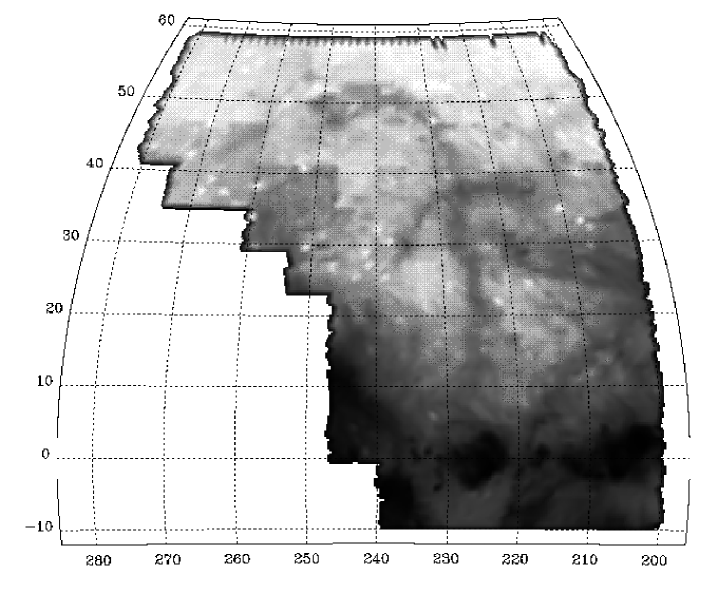
Figure 2.: An example of WHAM’s survey data. The 10^∘$\times$10^∘region centered on (l,b)=(215.8^∘,30.2^∘) is shown at higher angular resolution in Fig. 6. Adapted from Haffner et al. (1998), reprinted by permission.

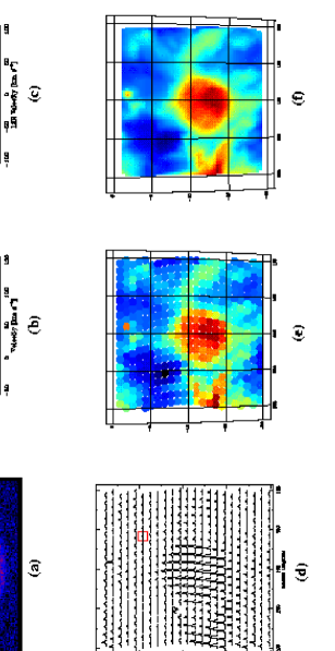
Figure 3.: Steps in processing WHAM data. (a) The CCD data from one beam on the sky. Each ring corresponds to line emission at a different velocity. The radial velocity decreases from center to edge. (b) The spectrum is formed by azimuthally averaging the CCD data from (a). Velocity coverage is $\sim 200$ km s^-1, with resolution 12 km s^-1. (c) The calibrated spectrum includes flat fielding, baseline fitting, intensity and velocity calibration, and subtraction of the geocoronal line. (d) A grid of calibrated spectra. A small square highlights the example spectrum in the previous panels. (e) A grid of nested beams show the integrated light within the range V${}_{LSR}=-6$ to $+6$ km s^-1. (f) The final, rectilinear image results from oversampling and smoothing the data from panel (e). Reproduced in B&W, intensity does not map monotonically to grey scale. From Haffner (1998), reprinted by permission.

Figure 4.: Top: Careful component– and baseline-fitting is required to extract the Galactic H$\alpha$ emission from Fabry-Perot spectra. The Galactic H$\alpha$ spectrum is the thick solid line. Bottom: The Galactic H$\alpha$ spectrum is plotted again with a 20X expanded scale. The Galactic H$\alpha$ emission is 1.0 R, typical for high latitude regions. A Gaussian fit is plotted too. Reprinted by permission from Marcelin et al. (1998).

5.2. Narrowband Imaging

To make wide-field, narrowband images, an interference filter can be placed in front of a camera lens attached to a CCD. The interference filter typically is 10 to 50Å wide (FWHM). A narrow bandpass $\Delta\lambda$ is desirable to suppress continuum light from the night sky, ${{d\Sigma_{sky}}\over{d\lambda}}$, because the signal-to-noise ratio SNR of the H$\alpha$ light detected in time $\tau$ over a solid angle $\Omega$ is photon-limited if detector noise can be neglected:

$$SNR\mathrel{\hbox{\hbox to0.0pt{\hbox{\lower 4.0pt\hbox{$\sim$}}\hss}\hbox{$<$}}}\tau~{}\Omega~{}\Sigma_{\alpha}/\sqrt{\tau~{}\Omega~{}(\Delta\lambda~{}{{d\Sigma_{sky}}\over{d\lambda}}~{}+\Sigma_{\alpha})}.$$ (5)

However, the narrower the bandpass, the narrower is the usable field of view, because the central wavelength $\lambda$ of an interference filter shifts blueward by ${\delta}\lambda$ as the angle of incidence $\theta$ increases,

$${\delta}\lambda\approx-\lambda~{}{{sin^{2}(\theta)}\over{2~{}n^{2}}},$$ (6)

where $n$ is the index of refraction of the filter ($n\approx 2$). Equation 6 implies that the usable solid angle $\theta^{2}$ is approximately proportional to filter width $\Delta\lambda$. Equation 5 implies that to detect H$\alpha$ signals that are much fainter than the continuum, the time required is proportional to the filter width: $\tau\propto\Delta\lambda$. Thus, a narrowband imaging survey can be made as quickly with a wide filter and wide field of view as a narrow filter and narrow field of view. Wide filters require extremely precise gain calibration (i.e. flat-fielding) to see the small fraction of the light that is H$\alpha$. On the other hand, narrow fields of view result in more images to mosaic. This analysis breaks down at very wide filters ($\Delta\lambda\mathrel{\hbox{\hbox to0.0pt{\hbox{\lower 4.0pt\hbox{$\sim$}}\hss}\hbox{$>$}}}50$ Å) because telluric emission lines (primarily those of OH at 6554 Å and 6577 Å) increase the brightness of the sky. Similarly, the analysis breaks down for very narrow filters ($\Delta\lambda\mathrel{\hbox{\hbox to0.0pt{\hbox{\lower 4.0pt\hbox{$\sim$}}\hss}\hbox{$<$}}}5$ Å) because the geocoronal H$\alpha$ emission begins to exceed the sky continuum ($\Sigma_{\alpha,geo}\mathrel{\hbox{\hbox to0.0pt{\hbox{\lower 4.0pt\hbox{$\sim$}}\hss}\hbox{$>$}}}~{}\Delta\lambda{{d\Sigma_{sky}}\over{d\lambda}}$).

The narrowband imaging technique was applied to a large field of view by McCullough, Reach, & Treffers (1990) to create a 70^∘$\times$45^∘H$\alpha$ mosaic near the Galactic anticenter (Fig. 5). They used a $320\times 512$ pixel RCA CCD, a 50-mm lens, and a 44Å wide H$\alpha$ filter at a light-polluted site. Their wide-field H$\alpha$ mosaic revealed H II regions in the Galactic plane and filamentary structures at moderate Galactic latitudes. The mosaic also shows the edges of the individual images; they are prominent because the median value of each image was forced to zero by subtracting a constant, rather than a more sophisticated method such as globally fitting and individually subtracting a set of polynomials matched to the background of each image.

Gaustad, Rosing, McCullough, & Van Buren (1998) have installed a robotic camera at Cerro Tololo Inter-american Observatory in Chile (www.astronomy. swarthmore.edu). The robotic mount and dome point and protect the camera with almost zero assistance. In nominal operation, the robot requires human interaction for three operations: 1) if its weather monitor indicates that conditions are fine to open the dome, the robot confirms that with the 4-m telescope operator by email, 2) the 4-m operator also may tell the robot to close its dome at any time if conditions warrant, and 3) each week a human inserts a blank tape and mails a full tape to the USA for analysis.

The thermoelectrically cooled 1024$\times$1024 CCD has 12 $\mu$m pixels. Coupled to a Canon lens of 50-mm focal length, the CCD yields a field of view of 13^∘$\times$13^∘and a scale of 0.8^′ per pixel. (The 30-mm diameter aperture is similar to the apertures of Galileo’s first telescopes!) Images are taken through a 30Å wide H$\alpha$ filter and a dual-bandpass filter that excludes H$\alpha$ but transmits two 60Å bands of continuum light, one on each side of H$\alpha$. The filters are enclosed in an insulated, thermostated wheel to prevent drifts in the transmission curves. Because twilight sky is inadequately flat over wide fields of view (Chromey & Hasselbacher 1996), flat-fielding is accomplished with a custom light box with both incandescent and H$\alpha$ lamps.

The robotic imaging survey consists of 269 fields covering the sky from declination -90^∘ to +15^∘, with the same centers as those in the IRAS Sky Survey Atlas. Each field is observed six times in continuum (5 minutes per exposure) and five times in H$\alpha$ (20 minutes per exposure). The H$\alpha$ images are interleaved between the continuum images to minimize differences in the continuum level between the two as the zenith angle changes. Multiple exposures also permit rejection of cosmic rays, airplanes, and satellites. Figure 6 illustrates the image processing. Sensitivity is maximized at angular scales from 0.1^∘ to 2^∘, with much smaller features being limited by shot-noise and residuals of star-subtraction, and much larger features being difficult to distinguish from variations in the foreground sky and flat-fielding errors. Structures of angular extent 0.1^∘ to 2^∘and surface brightnesses of $\mathrel{\hbox{\hbox to0.0pt{\hbox{\lower 4.0pt\hbox{$\sim$}}\hss}\hbox{$>$}}}$1 R are detected reliably in the final images.

Because the 13^∘$\times$13^∘ images are spaced by 10^∘, every spot within 3^∘ of the edge of any image appears on an adjacent image also (the corners appear 4 times). This redundancy is helpful in mosaicing images and in recognizing genuine Galactic H$\alpha$ emission. Some fields were missed in the first year of observing. Those fields are the highest priority of the second year, with the remaining time allocated to observing a second grid of positions offset from the first grid by 5^∘. As of February 1999, 234 (87%) of the fields had been observed, with most of the missing fields at declination $\delta\geq 0$^∘.

Another imaging survey has been conducted by Dennison, Simonetti, & Topasna (1998). Their cryogenically-cooled CCD camera has a 58-mm lens, 27 $\mu$m pixels, a scale of 1.6^′/pixel, and covers a 13.6^∘$\times$13.6^∘field of view. They have observed much of the Milky Way ($|b|\mathrel{\hbox{\hbox to0.0pt{\hbox{\lower 4.0pt\hbox{$\sim$}}\hss}\hbox{$<$}}}30$^∘) from southwestern Virginia.

Galactic plane or low-latitude observations probably are not relevant to the CMB-foreground problem only because all foregrounds are too strong at low latitudes to permit templates to be subtracted accurately. The H$\alpha$ survey of Buxton, Bessell, & Watson (1998) and the Br$-\gamma$ (2.1655 $\mu$m) observations of Kutyrev et al. (1997) are in that category. However, Br$-\gamma$ is a good alternative to H$\alpha$  wherever dust extinction is significant, i.e. primarily at low latitudes.

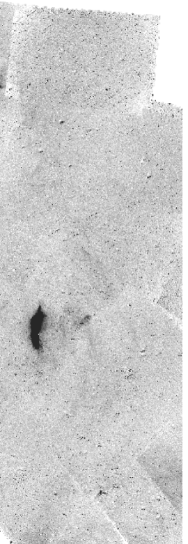
Figure 5.: Imaged in H$\alpha$, the Galactic anticenter region shows classic Stromgren spheres in the Galactic plane, and filaments of ionized gas at moderate latitudes. The region displayed extends from l = 120^∘ to 190^∘, b = -30^∘ to +15^∘and the limiting sensitivity is 4 R at 2^′ resolution. Adapted from McCullough, Reach & Treffers (1990).

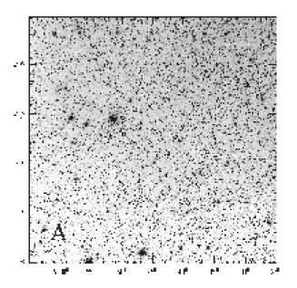
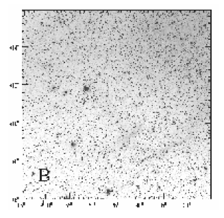
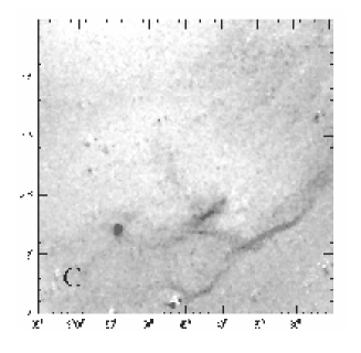
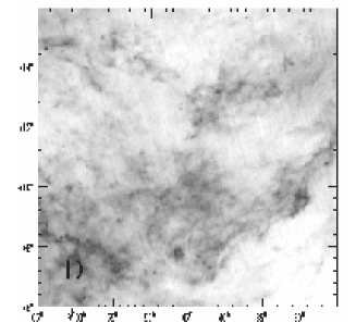
Figure 6.: The data processing steps for the imaging technique are outlined here with data from CTIO. A) A flat-fielded image made with a continuum filter. B) Same as A but with an H$\alpha$ filter. C) The difference image shows only H$\alpha$ emission and residuals around a few bright stars. This difference image results from 1) multiplying image A by a constant to match the stellar photometry of the two images A & B, 2) registering and subtracting the scaled image A from image B, 3) median filtering the result with a 7x7 pixel (5^′$\times$5^′) kernel to suppress residuals around stars, and finally fitting and subtracting an arbitrary first-order surface (a plane) to remove geocoronal emission. The bright source at 8$.\!\!^{\rm h}$55$.\!\!^{\rm m}$+9^∘is the planetary nebula A 31. D) The 100 $\mu$mIRAS ISSA image of the same region. The tendency for the H$\alpha$ emission to outline the dust emission is discussed in Section 6. The Galactic plane is toward the lower right (southwest).

6. Correlations

Dust and gas are well mixed in the ISM, so we might expect to see a positive correlation between dust emission and free-free emission. If instead the dust and gas in the ISM were like immiscible fluids such as oil and water, we might expect to see an anti-correlation, namely that where there is much dust (oil), there is little gas (water).

Some models of the ISM predict that neutral atomic hydrogen gas and ionized hydrogen gas are not well mixed but may be spatially and physically associated. For example, the model of McKee & Ostriker (1977) has H I clouds with H II skins surrounding them. As discussed below, H II skins around clouds are observed.

Reynolds et al. (1995) examined the relationship between H I and H II in velocity-resolved maps of H$\alpha$ and 21-cm emissions. They observed H$\alpha$ -emitting H I clouds and for those clouds measured the ratio I_α/N${}_{HI}\approx 20$ R/10²¹ cm^-2. They also noted that the ratio decreased systematically from $\sim 15$ R/10²¹ cm^-2 to $\sim 4$ R/10²¹ cm^-2 as the VLSR increased from -50 km s^-1 to 0 km s^-1, corresponding to a decrease in distance from the Galactic plane, $|z|$, from 1 kpc to 0 kpc. Converting from I_α/N_HI to I_α/I₁₀₀ with the factor ${\rm I_{100}/N_{H}=8.5~{}MJy~{}sr^{-1}/10^{21}cm^{-2}}$ typical for high latitude regions (Boulanger & Perault 1988), we find that Reynolds et al.’s results predict a range in slopes for the correlated components of H$\alpha$ and 100 $\mu$m emissions from 0.5 to 2.0 R / (MJy sr^-1). Kogut (1997) directly compared Reynolds et al.’s H$\alpha$ data with infrared data and derived an average ratio of I${}_{\alpha}/{\rm I_{100}}=0.85\pm 0.44$ R / (MJy sr^-1), which is within the range previously derived using the Boulanger & Perault factor.

Reynolds et al. found that the H$\alpha$ -emitting H I clouds account for only 30% of the H$\alpha$ emission and only 10% of the 21-cm emission. The amount of correlated emission is much less than the amount of uncorrelated emission. That is, the degree of correlation between H$\alpha$ and 21-cm emissions is not strong; it is weak, at angular scales less than a few degrees.

Figure 7 illustrates the meaning of the degree (or strength) of a correlation as compared with the slope of that correlation.

Figure 7.: The correlation between H$\alpha$ (or free-free) and dust emission is discussed in Section 6. In this figure, pairs of correlated random numbers illustrate the meaning of the degree (or strength) of a correlation and its slope. The label lists the correlation’s slope and its Pearson correlation coefficient. The latter quantifies the degree (or strength) of the correlation. The correlation is good (or strong) in the top panels and poor (weak) in the lower panels. The slope is four times larger in the right panels than the left panels. (To some people the fit in the lower left panel looks more accurate than the fit in the lower right panel, but that is an optical illusion: the data are identical except for a scale factor in Y.)

Table 2.: H$\alpha$ and Free-free Correlations with Dust^a

${\rm I_{\alpha}/I_{100}[R/(MJy~{}sr^{-1})]}$	Type	Source	Notes
$0.34\pm 0.33$	H$\alpha$	Kogut (1997)	b
$0.79^{+0.44}_{-0.15}$	H$\alpha$	McCullough (1997)	b
$0.85\pm 0.44$	H$\alpha$	Kogut (1997)	b
$0.5-2.0$	H$\alpha$	Reynolds et al. (1995)	c
$2.0\pm 0.5$	microwave	Kogut et al. (1996)	b
$3.6\pm 2$	microwave	de Oliveria-Costa et al. (1997)	b
$6$	microwave	Leitch et al. (1997)	b,c
$37\pm 19$	microwave	Lim et al. (1996)	d

Smoot (1998) has collected estimates of the slope of the correlation of H$\alpha$ and dust, and of free-free and dust; those are reproduced in Table 2. The aforementioned result, I${}_{\alpha}/{\rm I_{100}}=0.5$ to 2.0 R / (MJy sr^-1), and a result of Lim et al. (1996) are included also.

From data like those in Table 2, it has been noted that the H$\alpha$ observations imply less radio emission per unit dust emission than is observed in microwaves (Kogut 1997; Smoot 1998). If true, this might be evidence of an additional mechanism for microwave emission emanating from dust, perhaps of the sort described by Lazarian (in this volume) and plotted in Figure 1.

We can test the hypothesis that a single value for the ratio I${}_{\alpha}/{\rm I_{100}}$ is consistent with the data in Table 2. In doing so, we assume the measurements are not biased and that the error distributions are normal (a.k.a. Gaussian). As a practical matter, we do not include results that lack formal error estimates. The maximum likelihood value is 0.86 ($\pm$0.2) R / (MJy sr^-1). No individual result differs from the maximum likelihood value by more than 2.3 times the respective standard deviation. For the 6 measurements and 1 degree of freedom, the minimum $\chi^{2}=13.2$, which occurs 2% of the time by chance alone. The Lim et al (1996) result may be affected by anisotropy in the CMB (Kogut 1997), and if we disregard it, then for the 5 remaining measurements, the minimum $\chi^{2}=9.6$, which occurs 5% of the time by chance alone. Therefore, these data do not refute the hypothesis convincingly, especially if one considers the additional possibilities of bias in the means and non-Gaussian errors.

Kogut et al. (1996) report a good correlation between free-free emission and dust on $\mathrel{\hbox{\hbox to0.0pt{\hbox{\lower 4.0pt\hbox{$\sim$}}\hss}\hbox{$>$}}}7$^∘ angular scales observed with COBE’s DMR. McCullough (1997) reports a weak correlation between H$\alpha$ emission and dust on $\mathrel{\hbox{\hbox to0.0pt{\hbox{\lower 4.0pt\hbox{$\sim$}}\hss}\hbox{$<$}}}1$^∘ angular scales.

That the correlation weakens with decreasing angular scale can be understood with a simple geometric model in which neutral dusty clouds are externally ionized from a source emanating from the Galactic plane. A good example is shown in Figure 6C and D. The dust cloud has a “silver lining” of H$\alpha$ emission on the side of cloud nearest the Galactic plane. The same phenomenon is evident in another cloud at higher latitude (McCullough 1997).

The external ionization creates a skin of ionized gas preferentially on the side of the cloud nearest the Galactic plane. The narrowness of the H$\alpha$ lining indicates that the source of ionization doesn’t penetrate far into the cloud. (The 100 $\mu$m surface brightness implies A${}_{V}\leq 0.2$ mag, so H$\alpha$ light can pass through the cloud with minor attenuation.) If the surface of a cloud is uniformly ionized, for example by external photoionization, the “silver lining” effect will occur wherever the cloud’s surface is tangent to the line of sight, due to the longer path length. This model predicts that the degree of correlation between dust and ionized gas (observed by H$\alpha$ or free-free emission) will be A) weak on angular scales smaller than the size of a typical cloud but B) stronger on much larger angular scales.

Haffner et al. (1998) report WHAM data showing H$\alpha$ emission with little if any association with other emissions such as X-ray, infrared, or 21-cm. On the whole, narrowband images support this view, namely that in many cases, there is no obvious relationship between ionized gas and other constituents. However, in some case such as those discussed in the previous paragraphs, the detail revealed in the narrowband images clearly show a physical association. In other cases, the velocity revealed by spectroscopy is critical to our understanding.

7. Conclusions

Halpha observations completed in the past year will provide a template of the free-free emission from the Milky Way. The H$\alpha$ sky has been observed with a high-sensitivity Fabry-Perot spectrometer from the northern hemisphere, and with a narrowband imager from the southern hemisphere. Approximately 38% of the H$\alpha$ sky has been observed with both instruments. Both surveys are sufficiently sensitive to detect warm ionized hydrogen gas at all Galactic latitudes. A simple geometric model is proposed to explain observed correlations between ionized gas and dust.

Astronomers interested in the CMB will create maps that are free of free-free for free (i.e. without paying a noise penalty inherent in multi-frequency estimates of free-free emission). Alternatively, it may be possible to quantify the location and the brightness of another foreground such as that from rotating dust grains by comparing the H$\alpha$ template with the templates of synchrotron, free-free (directly-observed in microwaves), and thermal dust.

Acknowledgments.

We have benefited from the help of the WHAM team, in particular Matt Haffner, Ron Reynolds, and Steve Tufte. Students that have assisted us are Bender, Chen, Farney, Hall, Hentges, Khosrowshahi, Logan, Oh, Pulokas, Raschke, Schneider, Seaton, and Tajima. We also appreciate the assistance of the staff of CTIO in installing and maintaining our robot. The authors’ research has been supported by grants from the National Science Foundation, Las Cumbres Observatory, Dudley Observatory, the Fund for Astrophysical Research, the Research Corporation, NASA, Swarthmore College, and the University of Illinois at Urbana-Champaign. This work was performed in part at the Jet Propulsion Laboratory of the California Institute of Technology, which is operated under contract with the National Aeronautics and Space Administration.

References

Arny, T. 1989, S&T, 78, No. 3, 238

Barnard, E. E. 1896, MNRAS, 57, 10

Barnard, E. E. 1900, MNRAS, 60, 258

Barnard, E. E. 1928, ApJ, 67, 281

Bartlett, J., & Amram, P. 1998, in Proceedings of the Moriond Workshop “Fundamental Parameters in Cosmology”, xxx.lanl.gov/abs/astro-ph/9804330

Bennett, C. L, et al. 1992, ApJ, 396, L7

Boulanger, F. & Perault, M. 1988, ApJ, 330, 964

Broadfoot, A. L., & Kendall, K. R. 1968, J. Geophys. Res., 73, 426

Buxton, M., Bessell, M. & Watson, B. 1998, Pub. Astron. Soc. Australia, 15, 24

Chromey, F. R. & Hasselbacher, D. 1996, PASP, 108, 944

de Oliveria-Costa, A., Kogut, A., Devlin, M. J., Netterfield, C. B., Page, L. A., & Wollack, E. J. 1997 ApJ, 482, L17

Dennison, B., Simonetti, J. H., & Topasna, G. A. 1998, Pub. Astron. Soc. Australia, 15, 147

Draine, B. T. & Lazarian, A. 1998, ApJ, 494, L19

Finkbeiner, D. P. 1999, private communication and these proceedings.

Gaustad, J. E., McCullough, P. R. & Van Buren, D., 1996. PASP, 108, 351

Gaustad, J., Rosing, W., McCullough, P.R., & Van Buren, D. 1998, IAU Symposium 190, 58

Haffner, L. M. 1998, PhD Thesis, University of Wisconsin-Madison

Haffner, L. M., Reynolds, R. J., & Tufte, S. L. 1998, ApJ, 501, L83

Jackson, J. D. 1975, Classical Electrodynamics, John Wiley & Sons, New York

Kogut, A. 1997, AJ, 114, 1127

Kogut, A. et al. 1996, ApJ, 464 , L5

Kutyrev, A. S., Bennett, C. L., Moseley, S. H., Reynolds, R. J., & Roesler, F. L. (1997), BAAS, 191, 06.03

Leitch, E. M., Readhead, A. C. S., Pearson, T. J., & Myers, S. T. 1997, ApJ, 486, L23

Lim, M. A., et al. 1996, ApJ, 469, L69

Marcelin, M., Amram, P., Bartlett, J. G., Valls-Gabaud, D., & Balnchard, A. 1998, A&A, 338, 1

McCullough, P. R. 1997, AJ, 113, 2186

McCullough, P. R., Reach, W. T., & Treffers, R. R. 1990, BAAS, 22, 750

McKee, C. F., & Ostriker, J. P. 1977, ApJ, 218, 148

Mezger, P. G., & Henderson, A. P. 1967, ApJ, 147, 471

Nossal et al. 1993, J. Geophys. Res., 98, 3669

Osterbrock, D. E. 1989, Astrophysics of Gaseous Nebulae and Active Galactic Nuclei, University Science Books, Mill Valley

Parker, R. A. R., Gull, T. R., & Kirschner, R. P. 1979, An Emission-Line Survey of the Milky Way, NASA SP-434, (NASA: Washington DC)

Rairden, R. L., Frank, L. A., & Craven, J. D. 1986, J. Geophys. Res., 91, 13613

Reynolds, R. J. 1992, ApJ, 392, L35

Reynolds, R. J. 1993, in “Massive Stars: Their Lives in the Interstellar Medium,” edited by J. Cassinelli & E. Churchwell, (Astronomical Society of the Pacific, San Francisco), p. 338

Reynolds, R. J. 1998, private communication

Reynolds, R. J. 1990, in IAU Symp. The Galactic and Extragalactic Background Radiation, Eds. S. Bowyer & C. Leinert, Netherlands, p. 157

Reynolds, R. J., Tufte, S. L., Kung, D. T., McCullough, P. R., & Heiles, C. 1995, ApJ, 448, 715

Simonetti, J. H., Dennison, B., & Topasna, G. A. 1996, ApJ, 458, 1

Sivan, J. P. 1974, A&AS, 16, 163

Smoot, G. F. 1998, xxx.lanl.gov/abs/astro-ph/9801121

Souras, Z. 1989, S&T, 77, No. 2, 128

Tinsley, B. A. 1968, J. Geophys. Res., 73, 4139

Tufte, S. L. 1997, PhD Thesis, University of Wisconsin-Madison

Tufte, S. T., Reynolds, R. J., & Haffner, L. M. 1998, ApJ, 504, 773

Valls-Gabaud, D. 1998, Pub. Astron. Soc. Australia, 15, 111