The Color Distributions of Globular Clusters in Virgo Elliptical Galaxies

Abstract

This Letter presents the color distributions of the globular cluster (GC) systems of 12 Virgo elliptical galaxies, measured using data from the Hubble Space Telescope. Bright galaxies with large numbers of detected GC’s show two distinct cluster populations with mean $V-I$ colors near 1.01 and 1.26. The GC population of M86 is a clear exception; its color distribution shows a single sharp peak near $V-I=1.03.$ The absence of the red population in this galaxy, and the consistency of the peak colors in the others, may be indications of the origins of the two populations found in most bright elliptical galaxies.

1. Introduction

The first detection of bimodality in the globular cluster system of an elliptical galaxy was made by Zepf & Ashman (1993) using the photometry of the M49 globular cluster (GC) system taken by Couture et al. (1991). Better data with larger samples of clusters subsequently confirmed the detection ( Zepf et al. 1995) and added several galaxies to the list of galaxies with detected bimodal distributions. Additional studies ( Geisler et al. 1996, Neilsen, Tsvetanov & Ford 1998) show that the radial color gradients in the mean color of the globular clusters of M49 and M87 can be attributed to variations in the spatial distributions of the clusters contributing to each peak.

This spatially varying bimodal distribution was predicted by the merger model of Ashman & Zepf (1992), in which the blue clusters are those of spiral galaxies which merged to form the elliptical, and the red clusters formed during the mergers. Cote et al. (1998) have proposed an alternate model in which only the red population is truly associated with the host galaxy, while the blue clusters were formed in other (smaller) members of the galaxy cluster and were captured during mergers or stripped from their original hosts through interactions. Under this model, the red clusters are metal rich because the large mass of the galaxy prevents metals from escaping. The blue clusters now follow the gravitational potential of the cluster as a whole, which is strongly centered on the central giant ellipticals.

There are serious objections to both models. The Cote et al. (1998) model has difficulty explaining the rotation of the GC system of M87, seen by Kissler-Patig & Gebhardt (1998) in the data set of Cohen, Blakeslee, & Ryzhov (1998). Furthermore, the stellar metallicity of the halos of elliptical galaxies is higher than that expected by stripping models (Harris, Harris & McLaughlin 1998). The Ashman & Zepf (1992) model implies a correlation between the relative numbers of red and blue clusters and specific frequency in globular cluster systems, which is not seen.

By obtaining high precision color measurements of large, well defined samples of GC’s in elliptical galaxies located in different parts of a galaxy cluster, further tests of these models become possible. For both the merger model and the tidal stripping model, one would expect the color of the blue population to be roughly the same in all galaxies. In the tidal stripping model, the size of the galaxy is expected to determine the location of the red peak, so a correlation between the color of the red peak and the luminosity of the galaxy is to be expected. (This correlation may be masked if a significant fraction of the stars were obtained in mergers.) However, in the merger model the shape and location of the color peak is dependent on the details of the merger history, and one would expect significant variation among the sample.

2. Observations, Reduction and Analysis

The Hubble Space Telescope archive provided all of the data used in this study. The sample includes those elliptical galaxies in the Virgo cluster for which there are WFPC-2 observations with images in filters which approximate the $V$ and $I$ bands (F814W and F555W or F606W, respectively), and which are deep enough to see a significant fraction of the globular clusters in a galaxy at 15-20 Mpc. Table 1 lists the basic parameters of the data taken.

The raw data were calibrated using the WFPC2 pipeline procedure. The different exposures were then aligned, cosmic ray rejected, and combined using standard software.

The custom program SBFtool was used both to determine the amplitude of the surface brightness fluctuations and to detect, classify, and perform photometry on candidate objects in the images. First, we model the galaxy and sky background using a combination of ellipse fitting or spatial frequency filtering techniques. We mark groups of four or more adjacent pixels significantly brighter than the model and noise as potential object pixels. Sets of pixels consistent with the shape of a PSF or distant globular cluster convolved by a PSF form the set of candidate globular clusters.

Because globular clusters at the distance of Virgo are partially resolved in HST WFPC-2 images, simple aperture photometry becomes complicated; the aperture correction will vary from object to object. Instead, we fit the data to a library of model GC’s constructed using King profiles and PSF’s created using tinytim (Krist 1997), covering a range of both core and tidal radii. (For similar approaches to photometry on partially resolved globular clusters, see Grillmair et al. (1999) and Holtzman et al. (1996).) In central, high signal to noise $(S/N>30)$ pixels, where errors in the model fitting become significant compared to the noise, the flux is measured directly. The flux outside these pixels is estimated using the best fit model.

The remaining catalog still contains contaminating objects, particularly background galaxies. The removal of objects with colors outside of the range $0.5<V-I<1.5$ (where practically all globular clusters fall), highly asymmetric objects, and objects where the best fitting model provided a poor reduced $\chi^{2}$ fit significantly reduces the contamination. For the study of the color distribution, we consider only objects with signals greater than 3000 e^- in each filter. These objects are significantly above the detection threshold in both filters, and the uncertainty in the color of fainter objects due to counting statistics alone is significant. The bright magnitude cutoff reduces the smoothing of the color distribution due to measurement error, ensures that the catalog is complete down to a well defined limit, and minimizes contamination due to remaining background galaxies. In all data sets except NGC 4365, NGC 4660, and NGC 4458, this limit is fainter than the expected peak of the GC magnitude distribution. The limit in the M86 data set is close to the expected peak of the GC distribution.

The procedure outlined by Holtzman et al. (1995) guided the conversion of the measured flux in the HST filters to standard $V$ and $I$ magnitudes.

3. Results

Table 1Globular cluster, host galaxy, and data properties

		Host Galaxy		GC Population					exp. time (s)
Galaxy	M	Type	$B-V$	$m_{V,lim}$	NGC	p	Mode 1	Mode 2	F555W	F814W
NGC 4472 (M49)	-21.6	E2	0.96	24.1	239	0.000	0.99	1.25	1800	1800
NGC 4406 (M86)	-21.5	E3	0.93	24.4	118	0.563	1.02	1.15	1500	1500
NGC 4365	-21.5	E3	0.96	24.3	170	0.190	1.04	1.23	2200	2300
NGC 4649 (M60)	-21.4	E2	0.97	24.3	276	0.000	1.02	1.27	2100	2500
NGC 4486 (M87)	-21.4	E0	0.96	24.4	616	0.000	0.98	1.22	2400	2400
NGC 4552 (M89)	-20.3	E0	0.98	24.4	152	0.000	1.05	1.29	2400	1500
NGC 4621 (M59)	-20.2	E5	0.94	23.5	102	0.286	1.06	1.22	1050	1050
NGC 4473	-20.0	E5	0.96	24.1	107	0.075	0.99	1.20	1800	2000
NGC 4660	-19.4	E6	0.92	23.5	41	0.162	0.99	1.15	1000	850
NGC 4478	-18.9	E2	0.91	25.4	64	0.037	0.99	1.29	16800	16500
NGC 4458	-18.8	E0-1	0.86	23.7	17	0.000	0.83	1.16	1200	1040
NGC 4550	-18.4	SB0	0.88	23.7	25	0.099	0.97	1.30	1200	1200

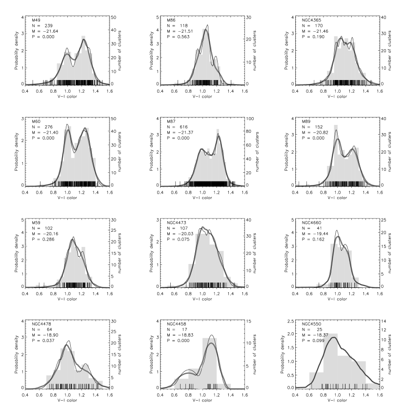
Figure 1.— Each plot shows the color distribution of globular clusters, together with the number of clusters used to create the distribution, the absolute magnitude of the parent galaxy based on the apparent magnitude as reported in RC3 and surface brightness fluctuations distance measurements for that galaxy, and the $p$ statistic from the KMM test. The filled grey area shows the histogram, and the lines show the distribution as estimated by a variable width Epanechnikov kernel with reference kernel widths which under-smooth (thin) and over-smooth (thick) the distribution. The ticks along the bottom represent the measured colors of the clusters in the sample.

Figure 1 displays the color distributions of each galaxy. The light grey shaded area shows the distribution using a traditional histogram. The histogram is not the ideal representation of the data; bin sizes narrow enough to detect fine structure will also display significant noise, and the choice of phase can also have a significant effect on the appearance. Simonoff (1996) describes and compares a variety of alternatives for estimating the underlying probability distribution, including the variable width Epanechnikov kernel.

For any given value, one of the simplest ways to measure the density of points at that value is to count the number of points within some distance $h$ of that value:

$$\hat{f}(x)=\sum_{i=1}^{n}\frac{1}{h}K(\frac{x-x_{i}}{h})$$

where

$$K(u)=\left\{\begin{array}[]{ll}\frac{1}{2}&\mbox{if $-1<u\leq 1$,}\\ 0&\mbox{otherwise.}\end{array}\right.$$

The appropriate choice of $h$ is a function both of the form of the underlying distribution and the density of data points; smaller values of $h$ are warranted when there are a larger number of data points. Use of an unnecessarily large value for $h$ will result in an overly smooth estimate of $f(x)$. One can accommodate the varying density of data points by substituting $h(x)=h_{\nu}\times f(x_{i})^{-\frac{1}{2}}$ for $h$. Clearly, an estimate of $f(x)$ must be made to apply this method, but an iterative process beginning with a crude (e.g., uniform) estimate provides stable results in few iterations. A second improvement that can be made is in the choice of the function $K(u)$. It can be shown that an estimate made using the Epanechnikov kernel,

$$K(u)=\left\{\begin{array}[]{ll}\frac{3}{4}(1-u^{2})&\mbox{if $-1<u\leq 1$,}\\ 0&\mbox{otherwise,}\end{array}\right.$$

minimizes the mean integrated square difference between $f(x)$ and $\hat{f}(x)$, provided that $f^{\prime\prime}$ is continuous, $f^{\prime\prime\prime}$ is square integrable, and $K(u)\geq 0$ (Simonoff 1996).

In figure 1, we present the color distributions using a simple histogram and approximations made using two values of reference kernel width, $h_{\nu}$. The thick line is the smoothing using a reference kernel width that would be optimal for a Gaussian distribution with a standard deviation equal to that of the data, and estimated using a constant kernel width. This value will over-smooth the data when applied with a variable kernel width and $\hat{f}(x)<1$, particularly if the distribution is not Gaussian; features seen in this smoothing are very likely to be real. A Kolmogorov-Smirnov (K-S) test comparing this smoothed distribution to the data confirms that it is significantly over-smoothed. The thin line shows the smoothing using a kernel width such that the smoothed curve can be excluded by a K-S test at the 50% level, giving an indication of what the true distribution may be. However, features seen in this line cannot be reguarded as having been reliably detected.

The KMM algorithm (Ashman, Bird, & Zepf 1994) provides a statistical test for comparing the likelihood of the underlying distribution being a single or double Gaussian. The KMM algorithm returns a likelihood ratio test statistic, which is a measure of the improvement in the fit of a two Gaussian model over a single Gaussian one. From this we calculate the $p$ value, the probability of measuring this statistic from a single Gaussian distribution. Low $p$ values reject the hypothesis that the examined distribution resulted from single Gaussian distribution. They do not necessarily reject other (possibly unimodal) models for the distribution, however. Because the presence of contaminating objects outside the main distribution significantly reduces the effectiveness of the KMM algorithm, we have removed objects with colors far from the main distribution (which are probably contaminating background galaxies) from our sample before applying the KMM algorithm to our data (see Ashman et al. 1994 for a more complete discussion of the effects of such a truncation).

Table 1 presents the various physical properties of each galaxy, including the absolute $B$ magnitude (calculated using SBF distances and RC3 apparent magnitudes), $B-V$ color, and Hubble type; the $V$ magnitude cutoff and the total number of clusters considered in the color distribution; and the $p$ value statistic and distribution locations from the KMM algorithm (mode 1 and mode 2).

4. Discussion

For four of the eight data sets where a reasonably large number of clusters have been detected $(N>100)$, two peaks are clearly identifiable even where the data are over-smoothed. Furthermore, in each of these four cases the locations of the peaks are consistently near $V-I=1.01$ and $V-I=1.26$. NGC 4365, NGC 4473, and M59 show single peaks, broader than the individual peaks in galaxies with bimodal distributions; the data are consistent with the base distribution being either a single broad peak or two peaks to close to be resolved. Although a single Gaussian distribution for these galaxies cannot be excluded, the relatively low $p$ value and best peak values (for the two Gaussian fit) close to 1.01 and 1.26 are suggestive of bimodality. M86 features a large population of globular clusters, but the distribution appears smoothly unimodal with a peak of $V-I\simeq 1.03$. The width and color of the peak are comparable to the width and color of the blue peak in the bimodal galaxies. The difference seems to be its lack of a red peak. In other properties, such as its luminosity and X-ray emission, it is similar to other bright galaxies in the sample. The only other remarkable feature is that M86 is bluer than any of the bright galaxies. This may indicate that the processes which result in a detectable red peak in the GC population also redden the star light of the galaxy as a whole. We do not emphasize the remaining four populations $(N<100)$ both because of the reduced overall statistics and the fact that the small number of clusters increases the effect of contamination by background galaxies on the overall appearance of the distribution.

While the positions of the modes of the color distribution appear uniform, the relative contribution of each peak to the distribution does not. The lack of a red peak in M86, and the strength of the red peak in the remainder of the bright galaxies, is a dramatic illustration of this variation.

In the model where the red population if supposed to from with the host galaxy, and the blue population is collected from neighbors, the mass of the galaxy is reguarded as the cause for the high metallicity of the clusters which originated with the host galaxy, so one expect a significant variation in the position of the red peak with galaxy mass. Our data set shows no such trend, although the range of magnitudes may be too small for such a trend to be detected. Why the red peak should show such consistency is equally unclear in the merger model of formation, as the distribution of red clusters should vary depending in the details of the merger history of the galaxy. It is possible, though, that the breadth of the red peak hides multiple populations formed though mergers, which typically result in a similar overall peak.

References

- (1) Ashman, K. M., Bird, C. M., & Zepf, S. E. 1994, AJ, 108, 2348
- (2) Ashman, K. M., & Zepf, S. E. 1992, ApJ, 384, 50
- (3) Ashman, K. M., & Zepf, S. E., 1998 Globular Cluster Systems (Cambridge, Cambridge University Press)
- (4) Cohen, J. G., Blakeslee, J. P., & Ryzhov, A.. 1998, ApJ, 496, 808
- (5) Cohen, J. G., & Ryzhov, A. 1998, ApJ, 486, 230
- (6) Cote, P., Marzke, R. O., & West, M. J. 1998, ApJ, 501, 554
- (7) Couture, J., Harris, W. E., & Allwright, J. W. B., 1991, ApJ, 273, 97
- (8) de Vaucouleurs, G., de Vaucouleurs, A., Corwin Jr., H. G., Buta, R. J., Paturel, G., & Fouque, P. 1991, Third Reference Catalogue of Bright Galaxies, version 3.9 (RC3)
- (9) Forbes, D. A., Grillmair, C. J., Williger, G. M., Elson, R. A. W., Brodie, J. P. 1998, MNRAS, 293, 325
- (10) Grillmair, C. J., Forbes, D. A., Brodie, J. P., & Elson, R. A. W., 1999, AJ, 117, 167
- (11) Geisler, D., Lee, M. G., & Kim, E. 1996, AJ, 111, 1529
- (12) Harris, W. E., Harris, G. L., & McLaughlin, D. E., 1998, AJ, 115, 1801
- (13) Holtzman, J. A., Burrows, C. J., Casertano, C., Hester, J. J., Trauger, J. T., Watson, A. M., & Worthey, G. 1995, PASP, 107, 1065
- (14) Holtzman, J. A., Watson, A. M., Mould, J. R., Gallagher, J. S., III, Ballester, G. E., Burrows, C. J., et al. 1996, AJ, 112, 416
- (15) Kissler-Patig, M., & Gebhardt, K., 1998, AJ116, 2237
- (16) Kissler-Patig, M., Kohle, S., Hilker, M., Richtler, T., Infante, L., & Quintana, H. 1997, A&A319, 470
- (17) Kissler-Patig, M., Richtler, T., Storm, J., Della Valle, M., A&A, 327, 503
- (18) Krist, J. 1997, The Tiny Tim Users Manual, Version 4.4 (Baltimore: STScI)
- (19) Kundu, A., & Whitmore, B. C. 1998, AJ, 116, 2841
- (20) Neilsen, E. H., Jr., Tsvatanov, Z. I., & Ford, H. C., 1998 in Proceedings of the Ringberg workshop on M87, ed. H. J. Röser, & K. Meisenheimer (Berlin: Springer), in press
- (21) Ostrov, P., Geisler, D., & Forte, J. C., 1993, AJ, 105, 1762
- (22) Secker, J., Geisler, D., McLaughlin, D., & Harris, W. E. 1995, AJ, 109, 1019
- (23) Simonoff, J. S. 1996, in Smoothing Methods in Statistics (New York: Springer-Verlag)
- (24) Whitmore, B. C., Sparks, W. B., Lucas, R. A., Macchetto, F. D., Biretta, J. A., 1995, ApJ, 454, 73
- (25) Zepf, S. E., & Ashman, K. M., 1993, MNRAS, 264, 611
- (26) Zepf, S. E., Carter, D., Sharples, R. M., & Ashman, K. M., 1995, ApJ, 445, 19