Observational Tests of the Mass-Temperature Relation for Galaxy Clusters

Abstract

We examine the relationship between the mass and x-ray gas temperature of galaxy clusters using data drawn from the literature. Simple theoretical arguments suggest that the mass of a cluster is related to the x-ray temperature as $M\propto T_{\rm x}^{3/2}$. Virial theorem mass estimates based on cluster galaxy velocity dispersions seem to be accurately described by this scaling with a normalization consistent with that predicted by the simulations of Evrard, Metzler, & Navarro (1996). X-ray mass estimates which employ spatially resolved temperature profiles also follow a $T_{\rm x}^{3/2}$ scaling although with a normalization about 40% lower than that of the fit to the virial masses. However, the isothermal $\beta$-model and x-ray surface brightness deprojection masses follow a steeper $\propto T_{\rm x}^{1.8-2.0}$ scaling. The steepness of the isothermal estimates is due to their implicitly assumed dark matter density profile of $\rho(r)\propto r^{-2}$ at large radii while observations and simulations suggest that clusters follow steeper profiles (e.g., $\rho(r)\propto r^{-2.4}$).

1 Introduction

The relationship between the mass and x-ray temperature of galaxy clusters is a necessary bridge between theoretical Press-Schechter models, which give the mass function (MF) of clusters, and the observed x-ray temperature function (TF) (e.g., Edge et al. (1990); Henry & Arnaud (1991); Henry (1997); Markevitch (1998)). Theoretical arguments suggest that the virial mass of a galaxy cluster is simply related to its x-ray temperature as $M\propto T_{\rm x}^{3/2}$. These arguments are supported by simulations which show a tight correlation between mass and temperature (e.g., Evrard, Metzler, & Navarro (1996); Bryan & Norman (1998); Eke, Navarro, & Frenk (1998)). This suggests that the M–T relationship may also be a relatively accurate and easy way to estimate cluster mass. However, the M–T relationship first needs to be calibrated using masses estimated by some other means.

The oldest method of measuring cluster mass is the virial mass estimate based on dynamical analysis of the observed velocity dispersion of the cluster galaxies. The existence of the x-ray emitting ICM of galaxy clusters allows an independent mass estimate but requires knowledge or assumptions about both the x-ray temperature and surface brightness profiles. More recently, strong and weak gravitational lensing by clusters has provided a third independent mass estimate. If clusters are dynamically relaxed and relatively unaffected by non-gravitational process, these three methods should give the same results. In this paper, we concentrate on virial and x-ray mass estimates.

In Section 2, we discuss the theoretical basis of the M–T relation and the results of cluster simulations. We then compare this relation with those using masses based on galaxy velocity dispersions (Section 3), x-ray mass estimates of clusters with spatially resolved x-ray temperature profiles (Section 4.1), and isothermal x-ray mass estimates ($\beta$-model estimates in Section 4.2 and surface brightness deprojection in Section 4.3). In Section 5, we discuss the results and present conclusions.

2 Theory and Simulations

For gas that shock heats on collapse to the virial temperature of the gravitational potential, the average x-ray temperature

$$T_{\rm x}\propto\frac{M_{\rm vir}}{r_{\rm vir}}\propto M_{\rm vir}^{2/3}$$ (1)

where $r_{\rm vir}$ is the virial radius, the boundary separating the material which is close to hydrostatic equilibrium from the matter which is still infalling. The coefficient of this relationship is a complicated function of cosmological model and density profile of the cluster (see e.g., Lilje (1992)). However, because the infall occurs on a gravitational timescale $t_{\rm grav}\propto\rho^{-1/2}$, the virial radius should occur at a fixed value of the density contrast, defined as:

$$\delta=\frac{\overline{\rho(r)}}{\rho_{c}(z)}=\frac{M(<r)}{\frac{4}{3}\pi\rho_{c}(z)r^{3}}$$ (2)

where $\rho_{c}(z)$ is the critical density. For an $\Omega_{0}=1$ universe, $\delta_{\rm vir}=18\pi^{2}\approx 178$ but drops to lower density contrasts for lower values of $\Omega_{0}$ (e.g., Lacey & Cole (1993)). Since we do not have a priori knowledge of the actual value of $\delta_{\rm vir}$, we scale all of our results to $\delta$ = 200, which should contain only virialized material, and has been used previously by other authors (e.g., Carlberg et al. (1996); Navarro, Frenk, & White (1995)).

Evrard et al. (1996) (hereafter EMN) present a M–T relation which seems to well describe simulated clusters in six different cosmological models (two $\Omega_{0}=0.2$ and four $\Omega_{0}=1$ models, see their Table 1 for details). EMN assume that $M\propto T_{\rm x}^{3/2}$ and then fit the coefficient of the relationship at various density contrasts. For $\delta\approx 200$, the coefficient depends only weakly on $\Omega_{0}$, with a difference of $\approx 5$% between the $\Omega_{0}=0.2$ and $\Omega_{0}=1$ models while the difference rises to $\approx 40$% at $\delta=2500$.

From EMN’s Equation 9 and fitting the normalization using their Table 5 (excluding the $\delta=2500$ values but including both $\Omega_{0}=0.2$ and $\Omega_{0}=1$ points), the expression for mass as a function of temperature and density contrast is:

$$M(\delta,T_{\rm x})=(1.81\pm 0.23)\times 10^{14}\delta^{-0.266\pm 0.022}\left(\frac{T_{\rm x}}{{\rm keV}}\right)^{3/2}\ h^{-1}\ {\rm M_{\odot}}$$ (3)

where h is the Hubble constant in units of 100 km s^-1 Mpc^-1. Note that Equation 3 shows that clusters in the EMN simulations have dark matter density profiles $\rho(r)\propto r^{-2.4}$ in accordance with the effective slope of the universal density profile of Navarro, Frenk, & White (1996) in the relevant range of radii.

Other simulations using different cosmological models and codes generally give normalizations similar to Equation 3 to within $\lesssim 20$%. Eke et al. (1998) give masses and gas temperatures at a density contrast of 100 for their simulations of an $\Omega_{0}=0.3$ $\Omega_{\Lambda}=0.7$ model which are well described by Equation 3. Bryan & Norman (1998) give the M–T at $\delta=250$ for simulations using variety of cosmological models. Like EMN they find the normalization is fairly insensitive to the model used although their normalizations are about 20% higher. Lastly, Metzler & Evrard (1997) examine the differences between simulations of galaxy clusters with and without galactic winds. The M–T relation in the wind models is slightly steeper due to the energy injection, with a power law index $\sim 1.6$ and has temperatures about 20% higher at the low mass end.

A redshift dependence is introduced into the normalization of the M–T relation by the definition of density contrast since the critical density is a function of $\Omega$ and the redshift of formation (see e.g., Lilje (1992); Eke, Cole, & Frenk (1996); Voit & Donahue (1998)). This should not substantially affect our results as the samples considered consist mainly of low redshift ($z\lesssim 0.1$) objects and/or have scatter in the mass estimates considerably greater than the effect introduced by the redshift dependence.

Since we have restricted ourselves to low density contrasts and redshifts, we will not discuss gravitational lensing mass estimates. Lensing estimates are usually limited to high density contrasts $\delta\geq 3000$ (even for weak lensing) and to moderate-to-high redshifts. However, Hjorth, Oukbir, & Van Kampen (1998) have reported good agreement between the EMN relation and their sample of eight lensing clusters. They assume $M\propto T_{\rm x}^{3/2}$ and an $\Omega_{0}=1$ cosmology. Their best fit normalization is 0.82 $\pm$ 0.38 (rms dispersion) times the EMN normalization.

3 Virial Theorem Mass Estimates

Assuming that the galaxies are distributed similarly to the total mass, the virial mass of a cluster depends on the line of sight projected velocity dispersion of the galaxies, $\sigma_{p}$, and the virial radius, $r_{vir}$:

$$M_{vir}=\frac{3}{G}\sigma_{p}^{2}r_{vir}.$$ (4)

If the entire system is not included in the observational sample, as is common for galaxy clusters, Equation 4 overestimates the mass. The usual form of the virial theorem (2U + T = 0) should be modified to include the surface term (2U + T = 3PV) since the surface pressure reduces the amount of mass needed to keep the system in equilibrium (see Girardi et al. (1998); Carlberg et al. (1997)).

Girardi et al. (1998) (hereafter G98) have derived virial masses for 170 nearby clusters ($z\leq 0.15$) using data compiled from the literature and the ENACS data set Katgert et al. (1998). They define the virial radius to be $r_{vir}=0.002\sigma_{p}\ h^{-1}$ Mpc where $\sigma_{p}$ is in km s^-1 and consider only galaxies within this radius in the mass estimation. Their quoted masses are generally smaller than previous estimates by $\lesssim 40\%$ which they attribute to stronger rejection of interlopers and a correction factor of $\sim 19\%$ accounting for the surface term.

We have cross-correlated the G98 catalog with two catalogs of ASCA temperatures (Fukazawa (1997); Markevitch (1998)) to obtain a subsample of 30 clusters with at least 30 redshifts within $r_{vir}$. Fukazawa and Markevitch excluded the center of the clusters to minimize the effect of cooling flows on the derived temperature. In cases of multiple measurements, the temperatures generally agree within their quoted errors (usually $\lesssim$ 10%), and we have preferentially used the Fukazawa temperatures. This sample has few low temperature clusters, so we have analyzed the archival ASCA data of three additional G98 clusters (see Table Observational Tests of the Mass-Temperature Relation for Galaxy Clusters). Cooling flow effects are not important for these three clusters. Table Observational Tests of the Mass-Temperature Relation for Galaxy Clusters lists clusters in the final sample along with their adopted x-ray temperature (column 2), G98 virial radius (column 3), and virial mass (column 4).

The assumption that $r_{vir}=0.002\sigma_{p}$ is quite approximate, and the actual relation between $r_{vir}$ and $\sigma_{p}$ depends on the cosmological model. The density contrast of the G98 virial masses ($=M_{vir}/(4/3\pi r_{vir}^{3}\rho_{c})$) is generally less than 200 with a mean (and standard deviation) of $97\pm 23$. Assuming the dark matter density $\rho(r)\propto r^{-2.4}$ in the outer parts of the clusters, which both the EMN simulations and Girardi data (at least the galaxy distribution) seem to follow, we have rescaled their masses to $\delta=200$. Effectively this is just a change of normalization such that the rescaled masses are smaller than $M_{vir}$ by about 15% (with a standard deviation of about 5%).

Figure 1 shows the distribution of rescaled virial masses versus temperature for this subsample. A power law fit using the BCES bisector method of Akritas & Bershady (1996), which takes into account the errors in both variables and the possibility of intrinsic scatter, gives $M\propto T_{\rm x}^{1.71\pm 0.20}$ (all quoted errors are 1$\sigma$ unless otherwise stated), marginally inconsistent with the EMN relation. The seven most severe of the outliers in this plot are A119, A754, A1656 (Coma), A2256, A2319, A3558, and A2029. Except for A2029, all are known to contain complex velocity or temperature structure. We have marked these six clusters in gray in Figure 1. Removing these six clusters from the fit gives $M\propto T_{\rm x}^{1.53\pm 0.13}$ and a normalization consistent with the EMN relation (see Table 1). Further outlier removal or permutations of the temperatures (i.e. using Markevitch instead of Fukazawa temperatures) does not cause significant differences in the fit (e.g., power law index is changed by $\pm 0.05$). Given the relatively large scatter, more clusters with well measured temperatures, especially cooler/less massive clusters, are needed to further constrain the relationship between virial mass and x-ray temperature.

3.1 The Velocity Dispersion–Temperature Relation

To first order, $M_{vir}\propto\sigma^{3}$ since $M_{vir}\propto\sigma^{2}r_{vir}$ and $r_{vir}\propto\sigma$. Therefore, the virial mass–temperature relation is related to the more extensively discussed velocity dispersion–temperature ($\sigma$–$T_{\rm x}$) relation (e.g., Lubin & Bahcall (1993); Bird, Mushotzky, & Metzler (1995); Wu, Fang, & Xu (1998) and references therein). Figure 2 shows the $\sigma$ – $T_{\rm x}$ relation for our G98 subsample. Excluding the same six clusters as above as fit gives $\sigma\propto T_{\rm x}^{0.54\pm 0.03}$. This is consistent with the observed $M_{vir}\propto T_{\rm x}^{1.5\pm 0.1}$.

If galaxies and gas are both in equilibrium with the cluster potential and gravity is the only source of energy, $\sigma\propto T_{\rm x}^{1/2}$ (e.g., Bird et al. 1995). Our results are marginally steeper than this and consistent with many previous estimates (e.g., 0.61 $\pm$ 0.13 from Bird et al. 1995). However, our fit is shallower than the fit G98 give in their paper (0.62 $\pm$ 0.04) possibly due to improved x-ray temperatures since they use Einstein and Ginga temperatures from David et al. (1993) and White, Jones, & Forman (1997). However, our fit is definitely shallower than the 0.67 $\pm$ 0.09 found by Wu et al. (1998). While they draw a much larger sample (94 clusters) from the literature, their sample is heterogeneous and the quality of their data is unclear. In contrast, we are using only G98 derived velocity dispersion with greater than 30 member redshifts and precise ASCA temperatures.

3.2 Scatter in Virial Mass Estimator

The scatter in the virial mass estimator is expected to be quite large because of shot noise due to the finite number of galaxies in a cluster and projection effects due to contamination by background and foreground galaxies. The scatter in the observed virial mass–temperature relation is then a combination of the dispersion in the virial mass estimator (with respect to the true cluster mass) and any intrinsic dispersion in the M–T relation.

Figure 3 shows a histogram of the ratio of the rescaled virial masses ($M_{200}(G98)$) to the mass expected from the best fit relation ($M_{fit}$). The mean (or median) is approximately 1.0 with a standard deviation of 0.31. Figure 3 excludes the six outliers that were not fitted, including these clusters increases the standard deviation to 0.59. The expected scatter in the virial mass estimator has not been widely reported in the literature, but Fernley & Bhavsar (1984) find that in their simulations of galaxy clusters the ratio of the virial mass to true mass is $0.97\pm 0.36$ (1$\sigma$ standard deviation) after removing contaminating background and foreground galaxies. This predicted scatter is close to the observed scatter around the fit and suggests the dispersion in the virial mass – temperature relationship is primarily due to the scatter in the virial mass estimator.

This is further supported by the distribution of $M_{200}(G98)/M_{fit}$ as a function of the number of redshifts ($n_{z}$) used to calculate the virial mass (see Figure 4 which also includes clusters with less than 30 redshifts). The scatter is about a factor of 2 lower for clusters with $n_{z}\geq 80$. This is not surprising as a larger number of redshifts increases the accuracy of the virial mass estimator by decreasing the shot noise. Together with the results in Figure 3, this further indicates that the M-T relation must have very small intrinsic scatter.

4 X-ray Mass Estimates

X-ray mass estimates are based on the assumptions that the ICM is in hydrostatic equilibrium and supported solely by thermal pressure. With the further assumption of spherical symmetry, the gas density, temperature, and pressure are related to the mass by:

$$\frac{dP_{g}}{dr}=\rho_{g}\frac{GM(<r)}{r^{2}}$$ (5)

$$P_{g}=\frac{\rho_{g}kT_{x}}{\mu m_{p}}.$$ (6)

where k is Boltzmann’s constant, and $\mu m_{\rm p}$ is the mean molecular weight of the gas. The enclosed mass at a radius, r is then:

$$M(<r)=-\frac{kT_{\rm x}(r)}{G\mu m_{\rm p}}r\left[\frac{d\ log\ \rho_{g}(r)}{d\ log\ r}+\frac{d\ log\ T_{\rm x}(r)}{d\ log\ r}\right],$$ (7)

which depends on both the gas density and temperature profiles. The gas density is usually assumed to follow a $\beta$ profile:

$$\rho_{g}(r)=\rho_{g}(0)\left[1+\left(\frac{r}{r_{\rm c}}\right)^{2}\right]^{-3\beta/2}.$$ (8)

Historically, x-ray detectors have either had good spatial or spectral resolution but not both. Measuring the actual temperature profiles of clusters has really only become practical with the advent of ASCA and its ability to obtain spatially resolved spectra. The combination of using ROSAT to obtain $\rho_{g}(r)$ and ASCA to obtain $T_{\rm x}(r)$ can yield cluster masses with unprecedented accuracy. However, estimating the temperature profile is complicated by the spatial and energy of the ASCA PSF, and mass estimates have only been reported for a few of the best observed clusters. The difficulty of measuring the temperature profiles means that there are far larger samples of clusters for which only the average x-ray temperature and isothermal mass estimates are available.

4.1 Mass Estimates with Spatially Resolved Temperature Profiles

No large catalog of clusters with masses measured using spatially resolved temperature profiles has been published. Therefore, we have searched the literature (including conference proceedings) to obtain a sample of 12 clusters with masses measured using known temperature profiles. These clusters are presented in Table Observational Tests of the Mass-Temperature Relation for Galaxy Clusters with the adopted average x-ray temperature and 90% confidence limits (column 2 or table notes), largest radius in which the mass was given (column 5), the mass within that radius (column 6), and the reference from which the data was taken (column 10). If given, we have used global temperature values given by the respective authors. Otherwise, we have taken them from catalogs of ASCA temperatures as in Section 3. The formal errors on these mass estimates are small as they are well constrained by the density and temperature profiles. However, the systematic uncertainties (i.e. uncertainties in the ASCA PSF and effective area) are much more difficult to quantify. For fitting purposes, we have chosen not to weight the fit with any mass errors, only with the errors in temperature.

Several of the clusters used warrant some comments. The masses for A496 and A2199 from Mushotzky et al. (1994) were derived without ASCA PSF corrections. However, the corrections are not large for these clusters as they are relatively cool and only the central field-of-view of the telescope was used. A2256 is known merger, but Markevitch & Vikhlinin (1997) argue that the subcluster is physically well separated along the line of sight and has not disturbed the bulk of the primary cluster’s gas. Although this cluster was considered an outlier in the virial mass fit, this can be attributed due to contamination of the optical velocity dispersion measurement.

As with the virial masses, we have rescaled the masses to a density contrast of 200 assuming the dark matter density profile $\rho(r)\propto r^{-2.4}$. On average, the effect of rescaling is to increase the masses by an average of 20% with a standard deviation of $\approx$25%. There is some support for using this profile. Markevitch et al. (1996) and Markevitch & Vikhlinin (1997) report similar profiles for A2163 and A2256. While other authors in Table Observational Tests of the Mass-Temperature Relation for Galaxy Clusters do not give density profiles, some (e.g., Ohashi (1997); Sarazin, Wise, & Markevitch (1998)) contain plots of the mass as a function of radius which are consistent with the $\rho(r)\propto r^{-2.4}$ profile. Lastly, the clusters themselves seem to obey this profile. Figure 6 show the density contrast (effectively the average density) as a function of radius. We normalize the radius to EMN’s $r_{200}$, the radius at which the density contrast is 200, so that we are comparing similar scales in different clusters but this makes little difference. An unweighted fit indicates that $\rho(r)\propto r^{-2.4\pm 0.1}$.

In Figure 5, we plot the rescaled masses versus temperature. Excluding A3526 (Centaurus), the best fit is $M\propto T_{\rm x}^{1.48\pm 0.12}$ but with a normalization about 40% lower than that of the EMN relation. Given the heterogeneous nature of the sample, the dispersion around this fit is surprisingly small ($\lesssim$ 10% in mass) indicating that the intrinsic correlation between temperature and mass is quite tight. Using a different density profile to extrapolate the mass to a density contrast of 200 has the tendency to increase the dispersion in this fit (i.e. about 25% for $\rho(r)\propto r^{-2}$) but does not have much effect on the power law index or normalization of the fit.

The lower normalization than that found using the EMN relation or virial masses may reflect systematics in the masses derived using the temperature profiles, or it could be a problem with the simulations and systematics in the virial mass determinations. Aceves & Perea (1998) have found that the virial mass estimate can either overestimate or underestimate the mass depending on the aperture of the region sampled. However, a direct comparison of the virial mass and x-ray masses for the 9 clusters with temperature profiles masses ($M_{200}(T(r))$) and G98 virial masses ($M_{200}(G98)$) (Figure 8) shows no clear trend. Further simulations and future observations of clusters with temperature profiles and virial masses will be need to explore this issue further.

4.2 The Isothermal $\beta$-model

The most often used x-ray mass estimator has been the isothermal $\beta$-model which assumes that the gas is isothermal and that the gas density follows Equation 8. Equation 7 then becomes:

$$M(<r)=1.13\times 10^{14}\beta\frac{T_{\rm x}}{{\rm keV}}\frac{r}{{\rm Mpc}}\frac{(r/r_{\rm c})^{2}}{1+(r/r_{\rm c})^{2}}M_{\odot}$$ (9)

assuming $\mu=0.59$. The $\beta$-model mass can be written in terms of density contrast (Equation 2) as:

$$M(\delta,\beta,T_{\rm x})=1.1\times 10^{15}\delta^{-1/2}\beta^{3/2}\left(\frac{T_{\rm x}}{{\rm keV}}\right)^{3/2}\left(1-0.01\frac{\delta r_{c}^{2}}{\beta T_{\rm x}}\right)^{3/2}h^{-1}M_{\odot}$$ (10)

We derive $\beta$-model masses using the data of Fukazawa (1997) (hereafter F97). In his study of the metal abundances and enrichment in the ICM, F97 presents a catalog of 38 clusters with temperatures, core radii, and $\beta$ parameters derived from ASCA data (see Table Observational Tests of the Mass-Temperature Relation for Galaxy Clusters columns 2, 7, and 8). F97 estimated the $\beta$ parameter from the ASCA GIS data using a Monte-Carlo method to take into account the spatial and energy dependence of the GIS PSF and estimated temperatures by excluding the central region of the x-ray emission to minimize cooling flow biases.

The F97 data has the advantage of being a homogeneous sample, although ASCA is not the best instrument for surface brightness fitting due to its complicated PSF. However, the ASCA GIS $\beta$-model fits are rather insensitive to the presence of cooling flows due to the high bandpass of the GIS. The clusters are also at low redshifts and so subtend a large area of the detector minimizing the effect of the poor resolution of the GIS. We compared the F97 $\beta$ values with those of derived from ROSAT studies (primarily using the PSPC) of David et al. (1995), Cirimele et al. (1997), and various others taken from the literature via the compilation of Arnaud & Evrard (1998) (see Figure 7 and Table Observational Tests of the Mass-Temperature Relation for Galaxy Clusters column 9). In general, they agree fairly well although ROSAT $\beta$ values are higher by an average of about 5%.

In Figure 5, we plot the estimated $\beta$-model mass at $\delta=200$ (using Equation 10) versus x-ray temperature. The relationship ($M\propto T_{\rm x}^{1.78\pm 0.05}$) is steeper than that seen using the EMN simulations, virial masses, or temperature profile masses. In addition, the relative normalization with respect to the other mass estimators is a function of density contrast. Increasing the density contrast shifts the $\beta$-model masses lower with respect to the EMN (or virial mass) relation and closer to the temperature profile masses while decreasing the density contrast has the opposite effect.

The isothermal $\beta$-model implicitly assumes a dark matter density profile of $\rho(r)\propto r^{-2}$ in the outer parts of clusters. The density profiles of clusters in the EMN simulations and clusters with measured temperature profiles generally seem to follow a steeper profile $\rho(r)\propto r^{-2.4}$ (see Section 4.1 and Figure 6). Therefore, the dark matter density profile implied by the isothermal $\beta$ model is probably not an accurate representation of clusters, and, despite the agreement of the $\beta$-profile with the observed gas density distribution, the different dark matter density profiles means that agreement between the isothermal $\beta$ model estimate and other mass estimates will be a function of radius (hence density contrast). The $\beta$-model masses underestimate the cluster mass at small radii and overestimate it at large radii. This has been pointed out previously by Bartelmann & Steinmetz (1996) and Markevitch et al. (1998). The different density profiles explain the relative steepness of the $M_{\beta}-T_{\rm x}$ relationship. For an individual cluster, $M_{\beta}/M(T(r))\propto r^{0.4}$. At any given density contrast, $r\propto T_{\rm x}^{1/2}$ and $M(T(r))\propto T_{\rm x}^{3/2}$, so the $\beta$ model mass within that overdensity would be $\propto T_{\rm x}^{1.7}$ similar to the fit given above.

4.2.1 Gas Density Profiles

Even if the underlying assumptions of the isothermal $\beta$-model are flawed, Equation 8 should still provide a good fit to the gas density distribution (see Suto, Sasaki, & Makino (1998) for a detailed discussion). The EMN relation is basically a $\beta$-model with $\beta=0.68$ for all clusters (depending on density contrast) regardless of x-ray temperature. However, the F97 data show a definite correlation of $\beta$ with $T_{\rm x}$ (see Figure 9). This indicates that the gas profile becomes shallower at lower masses. The relationship closely resembles that of the Metzler & Evrard (1997) models with galactic winds, although with a normalization 20% lower.

The variation of $\beta$ with $T_{\rm x}$ is unlikely to be an artifact of the F97 fitting procedure. As we noted in the previous section the F97 $\beta$ values generally agree with ROSAT values. The correlation of $\beta$ and $T_{\rm x}$ has also been noted previously in Einstein data David, Forman, & Jones (1991), and, more recently, Mohr & Evrard (1997) have found a similar trend for $\beta$ defined in a non-parametric and non-azimuthally averaged fashion using PSPC data. Arnaud & Evrard (1998) also note the behavior of $\beta$ with $T_{\rm x}$ and the discrepancy between the $\beta$-model and the expected EMN masses in their sample of clusters compiled from the literature. In fact, redoing the proceeding analysis with their sample gives virtually identical results.

4.3 Surface Brightness Deprojection

Another method for determining the mass of a cluster is x-ray image deprojection. The constraint of the observed surface brightness profile means that the profiles for the variables in Equation 5 & 6 can be determined by specifying one of them. The usual procedure is to divide the surface brightness emission into annuli. The outer pressure must be set in the outermost annuli (assumed to be due to gas not detected because its surface brightness is too low). The observed emissivity in the outer shell determines the temperature and hence the density. This procedure is then stepped inward and repeated. For more detailed discussion see Arnaud (1988), White et al. (hereafter WJF) and references therein.

WJF present an analysis of 207 clusters using an x-ray image deprojection analysis of Einstein IPC and HRI data to estimate the masses of clusters. WJF choose the functional form of the gravitational potential as two isothermal spheres, representing the central galaxy and general cluster potentials. These are parameterized by a velocity dispersion and core radius. For the central galaxy, these are fixed at 350 km s^-1 and 1 h^-1 kpc. The velocity dispersion of the cluster potential is taken from the literature or interpolated from the x-ray temperature or luminosity using an empirical relation. The core radius is a free parameter in the analysis which, with the outer pressure, is constrained to produce a flat temperature profile. Therefore, the derived gravitational mass depends on the velocity dispersion, x-ray surface brightness distribution, and temperature.

WJF determine the mass within the radius that they have x-ray data, which may be fairly small, while the EMN relation is only valid in the outer parts of the cluster (i.e. low values of density contrast). As with the G98 clusters, we can rescale the mass to a $\delta=200$, at least for the WJF clusters which have data in the outer parts of the cluster. We have rescaled the clusters with data at density contrasts ($=M_{WJF}/(4/3\pi r_{WJF}^{3}\rho_{c})$) less than 2000 to $\delta=200$ assuming $\rho(r)\propto r^{-2}$ as is the case for an isothermal sphere.

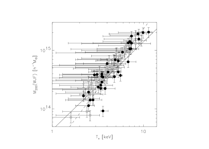
Figure 10: Mass–Temperature relation for WJF clusters using clusters with data for $\delta\leq 2000$. The solid circles are clusters which did not have any interpolated input data. The solid line is the theoretical EMN relation. The dashed line is a fit to the data. The error bars represent the 90% confidence intervals.

In Figure 10, we show the resulting $M_{200}$ versus $T_{\rm x}$ relation. Although the lower $T_{\rm x}$ error bars are quite large, allowing the the points to be statistically consistent with the EMN relation, the relation is obviously steeper. Fitting this relation using the BCES method gives a $M\propto T_{\rm x}^{2.06\pm 0.10}$ somewhat steeper than than found from the F97 data. The scatter in mass around this relation is also larger, about 50%.

Although WJF interpolated $\sigma$ or $T_{\rm x}$ for many clusters, using only the 45 clusters with data at $\delta<2000$ which did not have interpolated data does not alter our results. Also, the results reported using a subsample of 19 clusters with better determined parameters by White & Fabian (1995) are consistent with the WJF results. Furthermore, a recent deprojection analysis by Peres et al. (1998) of 45 clusters with ROSAT PSPC or HRI data gives a similar relationship as the WJF data, although the Peres et al. data are generally at higher density contrasts ($\gtrsim 3000$) making the extrapolation to $\delta=200$ even more uncertain.

Interpretation of the deprojection results is difficult as the derived gravitational masses are a combination of optical (the velocity dispersion) and x-ray data (the core radius and temperature). However, like the $\beta$-model masses the WJF masses follow a steeper relation due to the assumption of a potential which has a density profile which behaves as $\rho(r)\propto r^{-2}$. The large scatter is probably due to the use of the velocity dispersion to set the depth of the potential well.

5 Conclusions

We have examined the relationship between various galaxy cluster mass estimators and x-ray gas temperature. The resulting relationships generally agree to within $\lesssim 40$% in mass but with systematic offsets between different types of mass estimators. Using G98 virial masses and ASCA temperatures, we find good agreement with the EMN M–T relation after removing a few outliers. X-ray mass estimates using spatially resolved temperature profiles scale similarly but with a normalization about 40% lower. We note that the Hjorth, Oukbir, & Van Kampen (1998) lensing estimate mentioned at the end of Section 2 lies between these two estimates.

Mass estimates based on the assumption of isothermality like the $\beta$-model follow a steeper scaling relation due to the implicit assumption that the dark matter density scales $\rho(r)\propto r^{-2}$ at large radii while observational and numerical evidence suggests that clusters follow steeper profiles (i.e. $\rho(r)\propto r^{-2.4}$). As a consequence, the $\beta$ model underestimates the mass at low radii and overestimates it at large radii.

The intrinsic dispersion in the true M–T relationship is probably quite small. The scatter in the virial mass – temperature relation is consistent with most of the scatter being due to the dispersion in the virial mass estimator. The small scatter of the masses of clusters with spatially resolved temperature profiles also indicates that the dispersion in the M–T relation is probably $\lesssim$ 10%. More insight may be gained through simulations of projection effects on various mass estimators, but the most comprehensive study of these effects Cen (1997) is limited to fairly low masses clusters ($\lesssim 4\times 10^{14}h^{-1}M_{\odot}$ corresponding to $T_{\rm x}\lesssim 4$ keV). Simulations covering a larger mass range are necessary to better constrain the scatter in the M–T relation.

Our results also show that galaxy clusters seem to be affected by nongravitational processes such as energy injection by galactic winds. We find that $\beta$, the asymptotic slope of the gas density profile, is a function of temperature. The dependence is consistent with models of energy injection by galactic winds which tend to make the gas profile shallower in less massive clusters Mohr & Evrard (1997). The steepening of the $\sigma$–$T_{\rm x}$ relation is also consistent with energy injection by galactic winds (Bird et al. 1995). The good agreement between the virial and temperature resolved mass estimates and a $T_{\rm x}^{3/2}$ scaling law indicates that any temperature changes ($\Delta T$) due to energy injection must be small. However, meaningful constraints on $\Delta T$ are difficult given the relatively few clusters in this regime.

In the future, more optical virial mass estimates for cooler clusters and larger samples of clusters with resolved temperature profiles will enable better constraints on the M–T relation. Better x-ray data will allow the effect of energy injection on the apparent temperature and the spatial distribution of the ICM to be disentangled. Future x-ray observations (e.g., with AXAF) will produce both the gas density and temperature maps of clusters and allow maps of the gas entropy to be constructed which should produce new constraints on energy injection histories and entropy variations within the cluster population. Such entropy maps can then be compared with those produced from simulations of various heating mechanisms.

Figure 1: Virial Mass-Temperature relation. The solid line is the theoretical EMN relation while the dashed line is a fit to the G98 virial masses (rescaled to an density contrast of 200) and ASCA temperatures. The error bars represent the 90% confidence intervals for temperature and 68% confidence for mass. The gray circles indicate clusters excluded from the fit (named in the plot).

Figure 2: Velocity Dispersion-Temperature relation. The solid line is $\sigma\propto T_{\rm x}^{1/2}$. The dashed line is a fit to the data excluding the clusters marked in gray. The error bars represent the 90% confidence intervals for temperature and 68% confidence for velocity dispersion.

Figure 3: Histogram of virial to best fit masses excluding outliers.

Figure 4: Ratio of virial to best fit masses as function of number of redshifts used to calculate virial mass.

Figure 5: Mass–Temperature Relation. Filled circles are clusters with masses measured using spatially resolved temperature profiles rescaled to an density contrast of 200. The dashed line is a fit to this data. Gray diamonds are isothermal $\beta$-model masses within an overdensity of 200 for the F97 sample. The dotted line is the corresponding fit. The solid line is the theoretical EMN relation. Error bars are 90% confidence limits.

Figure 6: Density profiles of clusters with resolved temperature profiles as a function of radius, normalized to the EMN’s $r_{200}$. The solid line represents a fit to the data, $\delta\propto(r/r_{200})^{-2.4\pm 0.1}$.

Figure 7: Comparison F97 ASCA GIS $\beta$ values to ROSAT $\beta$ values. The circles are taken from David et al. (1995). The squares are from Cirimele et al. (1997), and the diamonds are taken from references listed in Arnaud & Evrard (1998).

Figure 8: Comparison of viral and temperature resolved mass estimates.

Figure 9: Relation between $\beta$ and $T_{\rm x}$ for F97 data. The dashed line is a fit to the data ($\beta\propto T^{0.26\pm 0.03}$).

Table 1: Fitting Results $M_{200}=c_{0}\times 10^{13}\ T_{\rm x}^{c_{1}}\ h^{-1}M_{\odot}$

Sample	$c_{0}$	$c_{1}$	Comments
EMN	$4.42\pm 0.56$	1.5
G98	$2.94\pm 0.80$	$1.71\pm 0.20$	all clusters
G98	$3.97\pm 0.76$	$1.53\pm 0.13$	excluding outliers
$M(T_{\rm x}(r))$	$2.72\pm 0.47$	$1.48\pm 0.12$
F97	$2.18\pm 0.14$	$1.78\pm 0.05$
WJF	$2.02\pm 0.29$	$2.06\pm 0.10$

Table 2: Cluster Data

Name	$T_{\rm x}$	$r_{\rm vir}$	$M_{\rm vir}$	$r_{\rm x}$	$M_{\rm x}$	$r_{c}$	$\beta$	$\beta_{ROSAT}$	Ref.
	keV	$h^{-1}$ Mpc	10${}^{14}h^{-1}M_{\odot}$	$h^{-1}$ Mpc	10${}^{14}h^{-1}M_{\odot}$	$h^{-1}$ Mpc
(1)	(2)	(3)	(4)	(5)	(6)	(7)	(8)	(9)	(10)
2A0335+096	3.01$\pm$0.07	$\cdots$	$\cdots$	0.50	1.10	0.023	0.60	$\cdots$	3
A0085	6.31$\pm$0.25	1.94	9.88${}_{-1.68}^{+2.25}$	$\cdots$	$\cdots$	0.086	0.60	0.62$\pm$0.03	10
A0119	5.59$\pm$0.27	1.36	2.50${}_{-0.74}^{+0.90}$	$\cdots$	$\cdots$	0.231	0.60	0.56$\pm$0.04	11
A0194	2.63$\pm$0.15	$\cdots$	$\cdots$	$\cdots$	$\cdots$	0.069	0.45	$\cdots$
A0262	2.15$\pm$0.06	1.05	1.32${}_{-0.25}^{+0.30}$	$\cdots$	$\cdots$	0.032	0.50	0.53$\pm$0.03	10
A0399	7.00$\pm$0.40	2.23	13.45${}_{-2.63}^{+2.74}$	$\cdots$	$\cdots$	$\cdots$	$\cdots$	$\cdots$	1
A0400	2.31$\pm$0.14	1.20	2.49${}_{-0.62}^{+0.73}$	$\cdots$	$\cdots$	0.051	0.45	$\cdots$
A0401	8.00$\pm$0.40	2.30	13.69${}_{-2.50}^{+2.76}$	$\cdots$	$\cdots$	$\cdots$	$\cdots$	$\cdots$	1
A0426	6.79$\pm$0.12	2.05	9.08${}_{-1.52}^{+2.13}$	$\cdots$	$\cdots$	0.020	0.45	$\cdots$
A0478	6.90$\pm$0.35	$\cdots$	$\cdots$	$\cdots$	$\cdots$	0.077	0.70	$\cdots$
A0496	4.13$\pm$0.08	1.37	3.20${}_{-0.95}^{+1.04}$	0.50	1.50	0.035	0.55	$\cdots$	4
A0539	3.24$\pm$0.09	1.26	2.01${}_{-0.42}^{+0.52}$	$\cdots$	$\cdots$	0.082	0.60	0.65$\pm$0.03	10
A0754	9.50$\pm$0.60	1.32	4.23${}_{-0.72}^{+1.04}$	$\cdots$	$\cdots$	$\cdots$	$\cdots$	$\cdots$	1
A1060	3.24$\pm$0.06	1.22	1.90${}_{-0.33}^{+0.38}$	1.00	1.80	0.040	0.55	0.61	5,9
A1656	8.38$\pm$0.34	$\cdots$	4.97${}_{-0.57}^{+0.68}$	$\cdots$	$\cdots$	0.208	0.75	0.75$\pm$0.03	9
A1795	5.88$\pm$0.14	1.67	5.86${}_{-1.22}^{+1.33}$	1.00	3.00	0.068	0.65	0.74$\pm$0.02	4,10
A2029	9.10$\pm$1.00	2.33	6.82${}_{-2.30}^{+2.40}$	0.96	4.71	$\cdots$	$\cdots$	$\cdots$	1,7
A2063	3.68$\pm$0.11	1.33	3.04${}_{-0.48}^{+0.59}$	$\cdots$	$\cdots$	0.067	0.60	0.67$\pm$0.04	10
A2107	3.78$\pm$0.19	1.24	2.62${}_{-0.77}^{+0.81}$	$\cdots$	$\cdots$	$\cdots$	$\cdots$	$\cdots$	2
A2142	9.70$\pm$1.30	2.26	17.84${}_{-3.49}^{+3.99}$	$\cdots$	$\cdots$	$\cdots$	$\cdots$	$\cdots$	1
A2147	4.91$\pm$0.28	$\cdots$	$\cdots$	$\cdots$	$\cdots$	0.109	0.50	$\cdots$
A2163	13.83$\pm$0.76	$\cdots$	$\cdots$	1.00	10.70	$\cdots$	$\cdots$	$\cdots$	8
A2199	4.10$\pm$0.08	1.60	5.71${}_{-1.21}^{+1.56}$	0.50	1.28	0.040	0.60	0.62$\pm$0.02	4,11
A2256	7.08$\pm$0.23	2.70	23.12${}_{-3.43}^{+3.95}$	1.50	6.00	0.228	0.75	0.81$\pm$0.01	6,9
A2319	8.90$\pm$0.34	3.09	39.54${}_{-5.12}^{+5.85}$	$\cdots$	$\cdots$	0.135	0.55	$\cdots$
A2634	3.70$\pm$0.28	1.40	4.31${}_{-0.98}^{+1.35}$	$\cdots$	$\cdots$	0.123	0.50	0.58$\pm$0.02	11
A2670	4.45$\pm$0.20	1.70	5.56${}_{-0.58}^{+0.72}$	$\cdots$	$\cdots$	$\cdots$	$\cdots$	$\cdots$	2
A3266	8.00$\pm$0.50	2.21	11.70${}_{-1.65}^{+1.96}$	$\cdots$	$\cdots$	$\cdots$	$\cdots$	$\cdots$	1
A3376	4.00$\pm$0.40	1.38	3.64${}_{-0.68}^{+0.78}$	$\cdots$	$\cdots$	$\cdots$	$\cdots$	$\cdots$	1
A3391	5.40$\pm$0.60	1.33	3.61${}_{-1.35}^{+2.20}$	$\cdots$	$\cdots$	$\cdots$	$\cdots$	$\cdots$	1
A3395	5.00$\pm$0.30	1.70	5.69${}_{-1.33}^{+1.58}$	$\cdots$	$\cdots$	$\cdots$	$\cdots$	$\cdots$	1
A3526	3.68$\pm$0.06	$\cdots$	$\cdots$	0.50	0.80	0.038	0.50	$\cdots$	3
A3558	5.12$\pm$0.20	1.95	11.54${}_{-0.91}^{+1.02}$	$\cdots$	$\cdots$	0.075	0.50	0.61	9
A3571	6.73$\pm$0.17	2.09	8.17${}_{-2.19}^{+2.40}$	$\cdots$	$\cdots$	0.086	0.60	$\cdots$
A3667	7.00$\pm$0.60	1.94	11.75${}_{-1.26}^{+1.60}$	$\cdots$	$\cdots$	$\cdots$	$\cdots$	$\cdots$	1
A4059	3.97$\pm$0.12	$\cdots$	$\cdots$	0.50	1.50	0.075	0.65	$\cdots$	3
AWM4	2.38$\pm$0.17	$\cdots$	$\cdots$	$\cdots$	$\cdots$	0.034	0.55	0.47
AWM7	3.75$\pm$0.09	1.73	5.77${}_{-1.50}^{+1.80}$	1.00	2.00	0.062	0.55	0.53$\pm$0.01	5,9
HCG51	1.23$\pm$0.06	$\cdots$	$\cdots$	$\cdots$	$\cdots$	0.058	0.55	$\cdots$
HCG62	1.05$\pm$0.02	$\cdots$	$\cdots$	$\cdots$	$\cdots$	0.003	0.40	$\cdots$
HYDRA-A	3.57$\pm$0.10	$\cdots$	$\cdots$	$\cdots$	$\cdots$	0.036	0.60	$\cdots$
MKW3S	3.68$\pm$0.09	$\cdots$	$\cdots$	1.00	2.00	0.047	0.65	$\cdots$	3
MKW4	1.71$\pm$0.09	1.05	1.15${}_{-0.26}^{+0.35}$	$\cdots$	$\cdots$	0.009	0.45	$\cdots$
MKW4S	1.95$\pm$0.17	$\cdots$	$\cdots$	$\cdots$	$\cdots$	0.023	0.40	$\cdots$
MKW9	2.23$\pm$0.13	$\cdots$	$\cdots$	$\cdots$	$\cdots$	0.025	0.45	$\cdots$
NGC2300	0.88$\pm$0.03	$\cdots$	$\cdots$	$\cdots$	$\cdots$	0.024	0.40	$\cdots$
NGC5044	1.07$\pm$0.01	$\cdots$	$\cdots$	$\cdots$	$\cdots$	0.009	0.50	$\cdots$
NGC507	1.26$\pm$0.07	$\cdots$	$\cdots$	$\cdots$	$\cdots$	0.014	0.45	$\cdots$
OPHIUCHUS	10.26$\pm$0.32	$\cdots$	$\cdots$	$\cdots$	$\cdots$	0.113	0.60	$\cdots$
S753	2.23$\pm$0.12	1.07	1.31${}_{-0.50}^{+0.67}$	$\cdots$	$\cdots$	$\cdots$	$\cdots$	$\cdots$	2
TRIAUST	10.05$\pm$0.69	$\cdots$	$\cdots$	$\cdots$	$\cdots$	0.126	0.60	0.63$\pm$0.02	9
VIRGO	2.58$\pm$0.03	1.26	2.04${}_{-0.21}^{+0.28}$	$\cdots$	$\cdots$	0.007	0.40	0.46	9

References. — (1) $T_{\rm x}$ from Markevitch (1998) (2) $T_{\rm x}$ derived for this paper (3) $M_{\rm x}$ & $r_{\rm x}$ from Ohashi (1997) (4) $M_{\rm x}$ & $r_{\rm x}$ from Mushotzky et al. (1994) (5) $M_{\rm x}$ & $r_{\rm x}$ from Loewenstein & Mushotzky (1996) (6) $M_{\rm x}$ & $r_{\rm x}$ from Markevitch & Vikhlinin (1997) (7) $M_{\rm x}$ & $r_{\rm x}$ from Sarazin, Wise, & Markevitch (1998), their value of $T_{\rm x}=8.69_{-0.36}^{+0.28}$ is used in Section 4.1 (8) $M_{\rm x}$ & $r_{\rm x}$ from Markevitch et al. (1996) (9) $\beta_{ROSAT}$ from Arnaud & Evrard (1998) (10) $\beta_{ROSAT}$ from David, Jones, & Forman (1995) (11) $\beta_{ROSAT}$ from Cirimele, Nesci, & Trevese (1997)

References

- Aceves & Perea (1998) Aceves, H., & Perea, J. 1998, in Observational Cosmology: The development of galaxy systems, eds. G. Giuricin et al., ASP Conference Series, in press
- Akritas & Bershady (1996) Akritas, M. G., & Bershady, M. A. 1996, ApJ, 470, 706
- Allen & Fabian (1998) Allen, S. W., & Fabian, A. C. 1998, MNRAS, 297, L57
- Arnaud (1988) Arnaud, K. A. 1988, in Cooling Flows in Clusters and Galaxies, ed. A. Fabian, 31
- Arnaud & Evrard (1998) Arnaud, M., & Evrard, A. E. 1998, preprint, astro-ph/9806353
- Bartelmann & Steinmetz (1996) Bartelmann, M., & Steinmetz, M. 1996, MNRAS, 283, 431
- Bird, Mushotzky, & Metzler (1995) Bird, C. M., Mushotzky, R. F., & Metzler, C. A. 1995, ApJ, 453, 40
- Briel, Henry, & Boehringer (1992) Briel, U. G., Henry, J. P., & Boehringer, H. 1992, A&A, 259, L31
- Bryan & Norman (1998) Bryan, G. L., & Norman, M. L. 1998, ApJ, 495, 80
- Carlberg et al. (1996) Carlberg, R. G., Yee, H. K. C., Ellingson, E., Abraham, R., Gravel, P., Morris, S., & Pritchet, C. J. 1996, ApJ, 462, 32
- Carlberg et al. (1997) Carlberg, R. G., et al. 1997, ApJ, 485, L13
- Cen (1997) Cen, R. 1997, ApJ, 485, 39
- Cirimele et al. (1997) Cirimele, G., Nesci, R., & Trevese, D. 1997, ApJ, 475, 11
- David, Forman, & Jones (1991) David, L. P., Forman, W., & Jones, C. 1991, ApJ, 380, 39
- David et al. (1995) David, L. P., Jones, C., & Forman, W. 1995, ApJ, 445, 578
- David et al. (1993) David, L. P., Slyz, A., Jones, C., Forman, W., Vrtilek, S. D., & Arnaud, K. A. 1993, ApJ, 412, 479
- Edge et al. (1990) Edge, A. C., Stewart, G. C., Fabian, A. C., & Arnaud, K. A. 1990, MNRAS, 245, 559
- Eke, Cole, & Frenk (1996) Eke, V. R., Cole, S., & Frenk, C. S. 1996, MNRAS, 282, 263
- Eke, Navarro, & Frenk (1998) Eke, V. R., Navarro, J. F., & Frenk, C. S. 1998, ApJ, 503, 569
- Evrard, Metzler, & Navarro (1996) Evrard, A. E., Metzler, C. A., & Navarro, J. F. 1996, ApJ, 469, 494
- Fernley & Bhavsar (1984) Fernley, J. A., & Bhavsar, S. P. 1984, MNRAS, 210, 883
- Fukazawa (1997) Fukazawa, Y. 1997, Ph.D. thesis, University of Tokyo
- Girardi et al. (1998) Girardi, M., Giuricin, G., Mardirossian, F., Mezzetti, M., & Boschin, W. 1998, ApJ, 505, 74
- Henry (1997) Henry, J. P. 1997, ApJ, 489, L1
- Henry & Arnaud (1991) Henry, J. P., & Arnaud, K. A. 1991, ApJ, 372, 410
- Hjorth, Oukbir, & Van Kampen (1998) Hjorth, J., Oukbir, J., & Van Kampen, E. 1998, MNRAS, 298, L1
- Katgert et al. (1998) Katgert, P., Mazure, A., Den Hartog, R., Adami, C., Biviano, A., & Perea, J. 1998, A&AS, 129, 399
- Lacey & Cole (1993) Lacey, C., & Cole, S. 1993, MNRAS, 262, 627
- Lilje (1992) Lilje, P. B. 1992, ApJ, 386, L33
- Loewenstein & Mushotzky (1996) Loewenstein, M., & Mushotzky, R. F. 1996, ApJ, 471, L83
- Lubin & Bahcall (1993) Lubin, L. M., & Bahcall, N. A. 1993, ApJ, 415, L17
- Markevitch (1998) Markevitch, M. 1998, ApJ, 504, 27
- Markevitch et al. (1998) Markevitch, M., Forman, W. R., Sarazin, C. L., & Vikhlinin, A. 1998, ApJ, 503, 77
- Markevitch et al. (1996) Markevitch, M., Mushotzky, R., Inoue, H., Yamashita, K., Furuzawa, A., & Tawara, Y. 1996, ApJ, 456, 437
- Markevitch & Vikhlinin (1997) Markevitch, M., & Vikhlinin, A. 1997, ApJ, 491, 467
- Metzler & Evrard (1997) Metzler, C., & Evrard, A. E. 1997, preprint, astro-ph/9710324
- Mohr & Evrard (1997) Mohr, J. J., & Evrard, A. E. 1997, ApJ, 491, 38
- Mushotzky et al. (1994) Mushotzky, R., Loewenstein, M., Arnaud, K., & Fukazawa, Y. 1994, in AIP Conference Proceedings, Vol. 336, Dark Matter, ed. S. S. Holt & C. L. Bennett (College Park, MD 1994: AIP), 231
- Navarro, Frenk, & White (1995) Navarro, J. F., Frenk, C. S., & White, S. D. M. 1995, MNRAS, 275, 720
- Navarro, Frenk, & White (1996) Navarro, J. F., Frenk, C. S., & White, S. D. M. 1996, ApJ, 462, 563
- Ohashi (1997) Ohashi, T. 1997, in ASCA/ROSAT Workshop of Clusters of Galaxies, ed. T. Ohashi (Hakone-Yumato: Japan Society for the Promotion of Science), 201
- Peres et al. (1998) Peres, C. B., Fabian, A. C., Edge, A. C., Allen, S. W., Johnstone, R. M., & White, D. A. 1998, MNRAS, 298, 416
- Sarazin, Wise, & Markevitch (1998) Sarazin, C. L., Wise, M. W., & Markevitch, M. L. 1998, ApJ, 498, 606
- Suto, Sasaki, & Makino (1998) Suto, Y., Sasaki, S., & Makino, N. 1998, ApJ, 509, 544
- Voit & Donahue (1998) Voit, G. M., & Donahue, M. 1998, ApJ, 500, L111
- White & Fabian (1995) White, D. A., & Fabian, A. C. 1995, MNRAS, 273, 72
- White, Jones, & Forman (1997) White, D. A., Jones, C., & Forman, W. 1997, MNRAS, 292, 419
- Wu, Fang, & Xu (1998) Wu, X.-P., Fang, L.-Z., & Xu, W. 1998, A&A, 338, 813