Dynamics of Line-Driven Winds from Disks in Cataclysmic Variables
I. Solution Topology and Wind Geometry

Abstract

We analyze the dynamics of 2-D stationary, line-driven winds from accretion disks in cataclysmic variable stars. The driving force is that of line radiation pressure, in the formalism developed by Castor, Abbott, & Klein for O stars. Our main assumption is that wind helical streamlines lie on straight cones.

We find that the Euler equation for the disk wind has two eigenvalues, the mass loss rate and the flow tilt angle with the disk. Both are calculated self-consistently. The wind is characterized by two distinct regions, an outer wind launched beyond four white dwarf radii from the rotation axis, and an inner wind launched within this radius. The inner wind is very steep, up to $80\arcdeg$ with the disk plane, while the outer wind has a typical tilt of $60\arcdeg$. In both cases the ray dispersion is small. We, therefore, confirm the bi-conical geometry of disk winds as suggested by observations and kinematical modeling. The wind collimation angle appears to be robust and depends only on the disk temperature stratification. The flow critical points lie high above the disk for the inner wind, but close to the disk photosphere for the outer wind. Comparison with existing kinematical and dynamical models is provided. Mass loss rates from the disk as well as wind velocity laws are discussed in a subsequent paper.

1 Introduction

Accretion disks are ubiquitous in astrophysical systems ranging from new-born stars to compact objects, like white dwarfs, neutron stars and black holes, both stellar and galactic. Due to their high temperatures and large surface areas, disks appear to be among the most luminous objects in the Universe. Strong dissipative processes which accompany accretion around compact objects can eleviate the radiation energy density in and above the disk, leading naturally to radiation-driven winds, similar to winds from hot stars. Observational signatures of such winds have been unambigously detected in cataclysmic variables (CVs) (Heap et al. 1978; Krautter et al. 1981; Klare et al. 1982; Córdova & Mason 1982) and in active galactic nuclei, hereafter AGNs (Arav, Shlosman, & Weymann 1997, and refs. therein), but their understanding proved to be challenging for theorists. In this and the following paper (Feldmeier, Shlosman, & Vitello 1999; hereafter Paper II) we focus on different aspects of disk winds in CVs, such as their 2-D geometry, solution topology, mass loss rates and velocity profiles. AGN disks will be discussed elsewhere.

Theoretical understanding of winds from accretion disks is hampered by their intrinsically multi-dimensional character and by the richness of various physical processes supplementing the basic hydrodynamics of the flow. A number of different driving mechanisms for disk winds have been predicted and analyzed, from magnetic torques to X-ray disk irradiation (i.e., Compton-heated and thermally-driven winds) to resonance line pressure (e.g., Blandford & Payne 1982; Begelman, McKee, & Shields 1983; Córdova & Mason 1985; Woods et al. 1996). Disks in non-magnetic CVs with high accretion rates, $\gtrsim 10^{-9}\,{\rm M}_{\odot}\,{\rm yr}^{-1}$, have an energy output which peaks in the (far-)ultraviolet, similarly to O, B and WR stars. Their spectra exhibit features which bear similarity to those found in hot and massive stars, and which are attributed to winds driven by radiation pressure in resonance and subordinate lines of abundant chemical elements, so-called line-driven winds (LDWs). Observational evidence in favor of LDWs winds from hot stars and disks includes but is not limited to the P Cygni line profiles of C iv, N v and Si iv, ionization levels, high terminal velocities and their correlation with the luminosity, and UV line behavior during continuum eclipse in CVs.

Pioneering works by Lucy & Solomon (1970), Castor (1974) and Castor, Abbott, & Klein (1975; CAK in the following) have shown that O star winds result from scattering of radiation in the resonance lines of abundant elements. Elegantly formulated theory of the LDWs from O stars by CAK, Cassinelli (1979), Abbott (1980, 1982), Pauldrach, Puls, & Kudritzki (1986) and others (for a textbook account, see Lamers & Cassinelli 1999), was successfully applied to individual objects. Further refinements of this theory by Owocki & Rybicki (1984, 1985) and Owocki, Castor, & Rybicki (1988) addressed the issue of stability of the flow.

First application of the LDWs to accretion disks (Shlosman, Vitello, & Shaviv 1985; Vitello & Shlosman 1988) emphasized the non-spherical ionizing continuum and driving force as well as a bi-conical geometry of the outflow. Under a broad range of conditions disk atmospheres in CVs and AGNs become dynamically unstable because the line opacity effectively brings them into a super-Eddington regime. Continuum photons absorbed by the UV resonance lines and re-emitted isotropically contribute to the momentum transfer to the wind. This process can be described as a resonant scattering which conserves the number of photons throughout the wind and results in terminal wind velocities of the order of the escape speed at the base of the flow.

The dynamics and radiation field of disk LDWs employed by Shlosman et al. (1985) and by Vitello & Shlosman (1988) were oversimplified. Both were approximated by a 1-D planar model allowing for divergence of the flow streamlines and geometrical dilution of the radiation field. Nineteen resonance lines in the range of $500-1,600$ Å were included in the calculation of the self-consistent radiation force. It was noted that disk LDWs are more restrictive than stellar winds and their development is strongly governed by the ionization structure in the wind.

Subsequently, a variety of 2-D kinematical models for disk winds in CVs supplemented by a 3-D radiation transfer in the Sobolev approximation were explored (Shlosman & Vitello 1993; Vitello & Shlosman 1993). Calculations using an alternative Monte Carlo radiation transfer method, albeit with frozen-in ionization, gave similar results (Knigge, Woods, & Drew 1995). Constrained by synthetic line profiles and by calculated effects of varying basic physical parameters, such as accretion and mass loss rates, temperature of the boundary layer, rotation, and inclination angle, the available phase space for wind solutions was sharply reduced. Wind resonant scattering regions exhibiting a strongly bi-conical character regardless of the assumed velocity and radiation fields were identified and mapped. This allowed to match the observed line shapes from a number of CVs and to put forward a number of predictions, which were verified in high-resolution HST observations (Shlosman, Vitello, & Mauche 1996; Mauche et al. 1999). Most importantly, rotation was positively identified as the dominant factor shaping the UV line profiles in CVs confirming that the disk and not the white dwarf is the wind source.

The above 1-D dynamical and 2-D kinematical modelings suffered from uniqueness problems which can be removed only by invoking the 2-D dynamics. Recent successful attempts by Proga, Stone, & Drew (1998; PSD hereafter) to model the 2-D time-dependent radiation hydrodynamics of disk LDWs was a major breakthrough in our understanding of this phenomenon. (The model of Murray & Chiang 1996 for CV winds, on the other hand, does not provide specifics for the wind geometry and hence we avoid discussing it here.) It confirmed basically that kinematical models of disk winds have sampled the correct parameter range and provided the scaling laws between different wind characteristics, e.g., between mass loss rate and accretion luminosity, and delineated the phase space for possible time-dependent solutions. A number of empirical relationships were put forward which require a physical explanation.

In this paper we focus on the 2-D geometry of a disk LDW in the presence of a realistic radiation field in CVs. We analyze solutions of the wind Euler equation, emphasising differences in the solution topology with that of CAK stellar winds. In the subsequent Paper II we address issues related to the mass loss rates and velocity laws of CV winds. The possible contribution to wind-driving by magnetic stresses is ignored here (e.g., Blandford & Payne 1982; Pudritz & Norman 1986; Emmering, Blandford, & Shlosman 1992), as are jet-like outflows seen in other disk systems (Livio 1997).

This paper is organized as follows. Section 2 reviews the relevant aspects of CAK theory for LDWs from O stars. Section 3 addresses the 2-D geometry of disk LDWs, as well as the radiation field above the CV disk. Section 4 deals with an analytic solution for vertical winds above an isothermal disk, and Section 5 analyzes the solution topology and flow geometry for tilted winds above a disk with a realistic temperature stratification. Section 6 compares our results with other models and observations, and Section 7 summarizes our work.

2 CAK theory for O stars

2.1 The stellar line force

The CAK theory for line-driven winds from O stars forms the basis for our model of CV winds, and is therefore briefly summarized here. CAK assume a line-distribution function per unit $\nu$ and $\kappa$, from UV to IR,

$$N(\nu,\kappa)={1\over\nu}\;{1\over\kappa_{0}}\;\left({\kappa_{0}\over\kappa}\right)^{2-\alpha},$$ (1)

where $\nu$ is the line frequency and $\kappa$ [${\rm cm^{2}\,g^{-1}}$] the mass absorption coefficient normalized to $\kappa_{0}$, where the latter refers roughly to the strongest driving line in the flow (Owocki et al. 1988). For the power exponent, $0<\alpha<1$ holds, where the lower limit corresponds to purely optically thin lines, and the (unrealistic) upper limit to purely optically thick lines. Puls, Springmann, & Lennon (1999) derive $\alpha=2/3$ from Kramers’ formula applied to resonance lines of hydrogenic ions. Similar values of $\alpha$ are obtained from detailed NLTE calculations for dense O supergiant winds (Pauldrach 1987; Pauldrach et al. 1994). On the other hand, for low-density winds, e.g., of B stars near-the-main sequence, $\alpha=1/2$ may be more appropriate (Puls, Springmann, & Owocki 1998). We shall, therefore, consider both cases $\alpha=1/2$ and $2/3$ to study the effect of $\alpha$ on the structure of disk winds.

Using eq. (1), the CAK force from all lines can be written in a general way applicable for both geometries (e.g., Owocki & Puls 1996),

$${\bf g}_{\rm L}=\kappa_{0}\,v_{\rm th}\;{\Gamma(\alpha)\over 1-\alpha}\;{1\over c^{2}}\int d\omega\;I_{\gamma}\;\mathbf{\hat{\gamma}}\;\tau_{\gamma}^{-\alpha},$$ (2)

by means of the Sobolev approximation (Sobolev 1957). $\Gamma(\alpha)$ is the complete Gamma function, $d\omega$ is a solid angle centered about $\mathbf{\hat{\gamma}}$, and $I_{\gamma}$ is the frequency-integrated intensity in this direction. The line optical depth in direction $\mathbf{\hat{\gamma}}$ is given by

$$\tau_{\gamma}={\kappa_{0}\,v_{\rm th}\,\rho\over\mathbf{\hat{\gamma}}\cdot\nabla(\mathbf{\hat{\gamma}}\cdot{\bf v})},$$ (3)

with gas density $\rho$, and $\mathbf{\hat{\gamma}}\cdot\nabla(\mathbf{\hat{\gamma}}\cdot{\bf v})$ being the gradient along $\mathbf{\hat{\gamma}}$ of the velocity component in direction $\mathbf{\hat{\gamma}}$. Note that $\kappa_{0}\,v_{\rm th}$ is independent of the ion thermal speed $v_{\rm th}$, and so is the line force. Assuming spherical symmetry, and adopting the ‘radial streaming’ approximation of CAK, i.e., $\tau_{\gamma}\equiv\tau_{r}$, eq. (2) simplifies to

$$g_{\rm L}=(\kappa_{0}\,v_{\rm th})^{1-\alpha}\;{\Gamma(\alpha)\over 1-\alpha}\;{F\over c^{2}}\;\left({dv/dr\over\rho}\right)^{\alpha},$$ (4)

with frequency-integrated, radial flux $F$.

2.2 Stellar Euler equation

For an isothermal, spherically symmetric stellar wind, the stationary Euler equation in dimensionless form can be written as,

$$\left(1-{A^{2}\over W}\right)W^{\prime}=-1-{4A^{2}\over U}+EW^{\prime\alpha},$$ (5)

where, after CAK, we introduced a radial coordinate $U=-R_{\ast}/r$, with $R_{\ast}$ being the stellar radius. The sound speed, $A$, and the flow speed, $V=\sqrt{W}$, are normalized to the photospheric escape speed from the reduced stellar mass, $M(1-\Gamma)$, where $\Gamma$ is the Eddington factor. The normalized wind acceleration is given by $W^{\prime}=dW/dU=$ $r^{2}vv^{\prime}/GM(1-\Gamma)$. Note that the gravitational acceleration is normalized to $-1$, whereas CAK normalize it to $-1/2$. The constant $E$ in (5) is given by

$$E={\Gamma(\alpha)\over 1-\alpha}\;\left[{\kappa_{0}\,v_{\rm th}\over 4\pi GM(1-\Gamma)}\right]^{1-\alpha}\;{L/c^{2}\over\dot{M}^{\alpha}},$$ (6)

where $L$ is the stellar luminosity and $\dot{M}$ is the mass loss rate, $\dot{M}=4\pi r^{2}\rho v$. Global solutions to (5) exist only above a certain, critical $E_{\rm c}$, called an eigenvalue of the problem, i.e., below a maximum allowable mass loss rate. In the zero-sound speed limit, $A=0$, the differential equation (5) separates into an algebraic equation,

$$P\equiv W^{\prime}+1-EW^{\prime\alpha}=0,$$ (7)

and a trivial differential equation $W^{\prime}=const$, which leads to the CAK velocity law, $v=v_{\infty}\sqrt{1-R_{\ast}/r}$, where $v_{\infty}$ is the flow terminal velocity. The Euler equation in the form (7) is particularly simple and its terms have a straightforward physical meaning, namely inertia, gravity and line force.

2.3 The stellar wind topology: critical point of the flow

We now consider solutions to eq. (5) with finite $A$. According to CAK, for sufficiently large values of $E$ there are two solutions in the supersonic regime, $W>A^{2}$, termed ‘shallow’ (small $W^{\prime}$) and ‘steep’ (large $W^{\prime}$) solutions, whereas in the subsonic, photospheric regime, $W<A^{2}$, only the shallow solutions exist. On the other hand, only the steep solutions reach infinity. Namely, the term $-4A^{2}/U$ (the thermal pressure force due to geometrical expansion) becomes infinite for $r\rightarrow\infty$, and must be balanced by $W^{\prime}\rightarrow\infty$ along the branch of steep solutions. CAK concluded therefore that the true, unique wind solution has to switch from the shallow to the steep branch at a ‘critical’ point (see Fig. 1). Of course, a non-zero pressure term at infinity is unphysical because it requires an infinite amount of energy in the flow and is purely a result of the imposed isothermal conditions in the wind.

The subsonic region has an extent of a few percent of the stellar radius for O star winds, while the pressure force $-4A^{2}/U$ becomes important only beyond a few $100\,R_{\ast}$. In the intermediate regime, i.e., almost everywhere, the simplified eq. (7) with $A=0$ holds to a good approximation, and therefore $W^{\prime}=const$. This happens since both gravity and line force are $\propto r^{-2}$. Solution curves in the $(W^{\prime},U)$ plane are essentially straight lines, bending over due to thermal pressure both at $U=-1$ and 0. As a result, the critical point is a saddle point in the $(W^{\prime},U)$ plane (Bjorkman 1995). The usual mathematical definition of a critical point refers, however, to the $(W,U)$ plane or a topologically equivalent plane.

For $A=0$, the critical point lies on an extended ridge, and its position becomes ill-defined (Fig. 1a). In this limit, every point of the critical solution is a critical point. For $A>0$, however, CAK find the critical point to lie at $r_{\rm c}={3\over 2}R_{\ast}$ (Fig. 1b). Inclusion of further correction terms to the line force, especially due to the finite size of the stellar disk, breaks the $r^{-2}$ dependence of the line force, pushes the two almost degenerate critical solutions $W^{\prime}(U)$ apart, and shifts the critical point towards the sonic point (Fig. 1c). Pauldrach et al. (1986) find then $r_{\rm c}\lesssim 1.1\,R_{\ast}$.

A critical point is the information barrier for LDWs, and plays a role similar to the sonic point in thermal winds or nozzle flows (Abbott 1980). How can the pressure mismatch of a shallow solution at $r\gtrsim 300\,R_{\ast}$ be communicated upstream to the critical point at $1.1\,R_{\ast}$? We speculate that it is not really the outer boundary mismatch which forces the flow through a critical point. Instead, the truly distinguishing property of the critical solution should be its correspondence to the maximum mass loss rate in the wind. Work is underway to identify the feedback mechanism between the wind and the photosphere which drives the wind from any shallow to the unique critical solution. This issue will be addressed elsewhere. In the present paper, we assume that the true disk wind solution is the one with the maximal allowable mass loss rate. Additional justification comes from the fact that only the shallow solutions for the disk wind connect to the disk photosphere. However, their terminal speeds are much smaller than the white dwarf escape speed, in sharp contrast to observed CV winds. The solution we are searching for should therefore switch to the steep branch (with large $v_{\infty}$) at some critical point, i.e., should be the solution of maximum mass loss rate.

The flow critical point (subscript ‘c’) is defined by the singularity condition, $\partial P/\partial W^{\prime}_{\rm c}=0$ (i.e., merging of a shallow and a steep solution). Together with the Euler equation, this implies

$$W^{\prime}_{\rm c} = {\alpha\over 1-\alpha},$$ (8a)

$$E_{\rm c} = {1\over\alpha^{\alpha}(1-\alpha)^{1-\alpha}}.$$ (8b)

The eigenvalue $E_{\rm c}$ determines the maximum mass loss rate, and $W^{\prime}_{\rm c}$ determines the terminal speed. They are further discussed in Paper II. Furthermore, from the Euler equation, $P=0$, also $dP/dU=0$ must hold everywhere. This leads to the regularity condition, $\partial P/\partial U_{\rm c}+W^{\prime}_{\rm c}\;\partial P/\partial W_{\rm c}=0$ (if $W_{\rm c}^{\prime\prime}<\infty$), which determines the position of the critical point.

3 Disk wind geometry and radiation field in CVs

3.1 Flow geometry, gravity and centrifugal force

The central assumption throughout this paper is that the helical streamline of a fluid parcel in the wind is contained within a straight cone. While this is certainly an idealization, and a major restriction of this model, justifaction comes firstly from the related kinematical model of Shlosman & Vitello (1993); and secondly from the numerical 2-D hydrodynamic simulations of PSD, which showed that the escaping mass-loss carrying streamlines are well approximated by straight lines in the $(r,z)$ plane, $r$ and $z$ being cylindrical coordinates.

We denote the angle between the wind cone and the radial direction ${\bf\hat{r}}$ in the disk plane by $\lambda$. This angle is calculated self-consistently using the Euler equation, and is not assumed a priori. The footpoint radius of a streamline in the disk is $r_{0}$, and $x$ is the distance along the cone (cf. Fig. 2). We search for the solutions of the Euler equation in the $[\lambda(r_{0}),x]$ plane, for a streamline starting at arbitrary $r_{0}$. The $\lambda(r_{0})$ dependence leads to the appearance of a new eigenvalue problem for the disk wind, and derivation of this function is the focus of the present paper.

Since LDWs are highly supersonic, we neglect the pressure forces, and furthermore assume that the azimuthal velocity is determined by angular momentum conservation above the disk, and by Keplerian rotation in the disk plane. The tilt angle $\lambda$ has to be a monotonically decreasing function of $r_{0}$ to avoid streamline crossing, which would violate the assumption of a pressureless gas. The only remaining velocity component is $v_{x}$, which points upwards along the cone. The dynamical problem has therefore been reduced to solving the Euler equation for $v_{x}$.

In a frame rotating with the angular velocity ${\bf\Omega}$ of a fluid parcel positioned at radius vector ${\bf r}$, there are three fictitious forces (e.g., Binney & Tremaine 1987). The Coriolis acceleration, $-2\;{\bf\Omega}\times\dot{\bf r}$, has no component along ${\bf\hat{x}}$, and the same is true for the inertial force of rotation, $-\,\dot{\bf\Omega}\times{\bf r}$. We introduce the effective gravity function, which is the component of gravity minus centrifugal force along the straight line in direction ${\bf\hat{x}}$, and is given by $-(G\,M_{\rm wd}/r_{0}^{2})\,g(X,\lambda)$, with $M_{\rm wd}$ being the mass of the white dwarf, and

$$g(X,\lambda)={X+\cos\lambda\over(1+2X\cos\lambda+X^{2})^{3/2}}-{\cos\lambda\over(1+X\cos\lambda)^{3}},$$ (9)

and $X\equiv x/r_{0}$. In the following, all lengths written in capital letters are normalized to the footpoint radius, $r_{0}$, in the disk. Close to the disk, $X\ll 1$, and $g\simeq X$, while for $X\gg 1$, $g\simeq X^{-2}$. For a vertical ray, $\lambda=90\arcdeg$, $g$ has its maximum at $X=1/\sqrt{2}$, while for a horizontal ray, $\lambda=0$, the maximum is at $X=1/2$.

Equation (9) shows an important difference between stellar and disk winds. The stellar gravity is always decreasing with distance, while for the disk an effective gravity ‘hill’ must be overcome before the wind can escape. This effect of disk LDWs will be discussed in Section 5.

3.2 Radiation field above the disk

Next, we evaluate the line force in eq. (2). Besides the initial growth of effective gravity with height, the opacity-weighted flux integral is the central property which distinguishes disk winds from stellar winds. Pereyra, Kallman, & Blondin (1997) give an analytical approximation for this integral above an isothermal disk. Unfortunately, an error was introduced with a change of integration variable, which led to an artificial, linear dependence of the vertical flux on $z$, even as $z\rightarrow 0$. PSD solve this integral numerically (cf. Icke 1980), using approximately 2,000 Gaussian integration points.

In the general spirit of the radial streaming approximation of CAK, we replace the integral in eq. (2) by $\bar{\tau}^{-\alpha}{\bf F}$, thus introducing an equivalent optical depth, $\bar{\tau}$. We first calculate the frequency-integrated flux $d{\bf F}(r,z)$ at location $(r,z)$ from a flat ring of radius $q$, radial width $dq$, and isotropic intensity $I(q,0)$,

$$d{\bf F}(r,z)=\left(\begin{array}[]{c}dF_{r}\\ dF_{z}\end{array}\right)=2\pi\,I(q,0)\,q\,dq\,{z\over B^{3/2}}\left(\begin{array}[]{c}r\bigl{[}r^{2}+z^{2}-q^{2}\bigr{]}\\ z\bigl{[}r^{2}+z^{2}+q^{2}\bigr{]}\end{array}\right),$$ (10)

where

$$B=\bigl{(}r^{2}+z^{2}-q^{2}\bigr{)}^{2}+4z^{2}q^{2}.$$ (11)

For an isothermal disk with isotropic intensity, we integrate eq. (10) over $q$, to obtain the disk flux

$${\bf F}(r,z)={\pi\,I\over 2}\;{1\over\sqrt{B}}\left.\left(\begin{array}[]{c}{\displaystyle z\over\displaystyle r}\bigl{[}r^{2}+z^{2}+q^{2}\bigr{)}]\\ -r^{2}-z^{2}+q^{2}\end{array}\right)\right|_{q=\,r_{\rm wd}}^{r_{\rm d}},$$ (12)

where $r_{\rm d}$ is the outer disk radius. For the nonmagnetic systems considered here, we identify the inner disk radius with $\,r_{\rm wd}$, the white dwarf radius. We do not include contributions to the radiative flux from the white dwarf and the boundary layer. Generally, of course, accretion disks are not isothermal. We, therefore, consider two complementary cases with $T(r_{0})\propto r_{0}^{-1/2}$ (termed ‘Newtonian’ disk in the following) and $T(r_{0})\propto r_{0}^{-3/4}\;\left(1-\sqrt{\,r_{\rm wd}/r_{0}}\right)^{1/4}$ (Shakura & Sunyaev 1973; SHS hereafter). Observations show that the brightness temperature stratification of CV disks is consistent with both these distributions (Horne & Stiening 1985; Horne & Cook 1985; Rutten et al. 1993).

For the Newtonian disk, we find

$${\bf F}(r,z)=\pi\,I(r)\,r^{2}\,{z\over r^{2}+z^{2}}\left.\left(\begin{array}[]{l}{\displaystyle 3r^{2}-z^{2}-q^{2}\over\displaystyle 2r\sqrt{B}}-{\displaystyle r\over\displaystyle z^{2}+r^{2}}\ln\;C\\ \phantom{0}\\ {\displaystyle 3z^{2}-r^{2}+q^{2}\over\displaystyle 2z\sqrt{B}}-{\displaystyle z\over\displaystyle z^{2}+r^{2}}\ln\;C\end{array}\right)\right|_{q=\,r_{\rm wd}}^{r_{\rm d}},$$ (13)

where

$$C={\displaystyle\bigl{(}z^{2}-r^{2}\bigr{)}q^{2}+\bigl{(}z^{2}+r^{2}\bigr{)}^{2}+\bigl{(}z^{2}+r^{2}\bigr{)}\sqrt{B}\over\displaystyle q^{2}}.$$ (14)

The surface flux above the SHS disk can only be integrated numerically, from eq. (10). Yet, this has the advantage that $\bar{\tau}$ can be introduced for each ring individually. More specifically, $\bar{\tau}$ is calculated along the flux direction of a given ring at the position of the wind parcel. If the flux (13) is used instead, $\bar{\tau}$ is calculated along the disk flux direction. Typical differences in the resulting value for the tilt angle $\lambda_{\rm c}$ (see below) are $5\arcdeg$ to $10\arcdeg$ for the two approaches. Corrections due to the $\tau^{-\alpha}$ weighting in the azimuthal integral are even smaller.

Figures 3 and 4 show isocontours for the $z$- and $r$-components of the flux (13) above the Newtonian disk. For sufficiently large tilt angles, the flux along the streamlines has a maximum larger than $\pi I(r_{0},0)$ at some $X$. This is due to the increasing visibility of the inner, hot disk regions. We denote this regime, where the flux has a maximum, the ‘panoramic’ regime, to be distinguished from the planar ‘disk’ regime, where $F_{z}\simeq\pi I$, and the ‘far field’ regime, where $F\propto X^{-2}$.

We now introduce the normalized flux, ${\bf{\tilde{F}}}(r,z)={\bf F}(r,z)/\pi I(r_{0},0)$, along a streamline, which is independent of disk luminosity. To quantify the flux increase above the disk, Fig. 5 shows the projected, normalized flux ${\tilde{F}}_{x}=$ ${\bf\hat{x}}\cdot{\bf{\tilde{F}}}$ as function of $X$, for different footpoint radii $r_{0}$ and for both types of non-isothermal disks. Note that the initial increase of ${\tilde{F}}_{x}$ with $X$ due to the wind’s exposure to the central disk region is rather mild, a factor of a few only, because the central region has a small area. In Section 5 we discuss how the maximum in ${\tilde{F}}_{x}$ controls the base extent of the wind above the disk, as well as the height of the wind critical point.

In deriving the above fluxes, the intensity was assumed to be isotropic. Using instead the Eddington limb darkening law, $I_{\theta}=\text@frac{2}{5}I_{0}\left(1+\text@frac{3}{2}\cos\theta\right)$, with polar angle $\theta$, the vertical flux in the planar disk regime above an isothermal disk becomes larger by a factor of 8/7, i.e., limb darkening should not significantly affect the wind properties. However, limb darkening can be more important in the UV spectral regime due to the Wien part of the spectrum, and the correction factors could become somewhat larger there (Diaz, Wade, & Hubeny 1996).

4 Vertical wind above an isothermal disk

As an analytically tractable case, we consider first a vertical (or cylindrical) wind with $\lambda=90\arcdeg$, or ${\bf\hat{x}}={\bf\hat{z}}$, above an infinite, isothermal disk with a flux ${\bf F}=\pi I\;{\bf\hat{z}}$. We again adopt the ‘radial streaming’ approximation in (2), i.e., $\bar{\tau}=\tau_{z}$. Note that $\tau_{z}$ has no contributions from either azimuthal velocity gradients, $\partial v_{\phi}/\partial r$, or from geometrical expansion terms, $\propto v_{\phi}$, the latter describing photon escape along the tangent to the helical streamline.

The density $\rho$ which enters $\tau$ is replaced by introducing the mass loss rate from one side of a disk annulus, $d\dot{M}$. Since the mass which streams upwards between two cylinders is conserved (using again coordinate $x$),

$$d\dot{M}(r_{0})=2\pi\,r_{0}\,dr_{0}\,v_{x}(r_{0},x)\,\rho(r_{0},x).$$ (15)

For simplicity, we apply the zero sound speed limit, $A=0$, for the rest of this paper, and neglect the force due to electron scattering because of small $\Gamma$ above the geometrically-thin disk. The Euler equation becomes

$$0=P(W^{\prime},X)=W^{\prime}+g-E\,W^{\prime\alpha},$$ (16)

where $g={X/(1+X^{2})^{3/2}}$ for $\lambda=90\arcdeg$, and $W^{\prime}=2V\,{dV/dX}$. Here $d/dX=r_{0}\;d/dx$, and $V$ is the flow speed normalized to the local escape speed at the footpoint $r_{0}$ on the disk. Normalizing instead to the escape speed from the white dwarf leads to unwanted, explicit appearances of $r_{0}$ in the Euler equation. The constant $E(r_{0})$ for a streamline starting at $r_{0}$ on the disk is defined as (compare with eq. 6)

$$E(r_{0})={\Gamma(\alpha)\over 1-\alpha}\;\left({\kappa_{0}\,v_{\rm th}\over 2\pi G\,M_{\rm wd}}\right)^{1-\alpha}\;{2\pi\,r_{0}^{2}\,F_{z}(r_{0},z=0)/c^{2}\over(r_{0}\;d\dot{M}(r_{0})/dr_{0})^{\alpha}}.$$ (17)

Similarly to the stellar case, eq. (16) for the disk wind has solutions only above a critical value $E_{\rm c}$, the eigenvalue of the problem, i.e., below a maximum allowable mass loss rate. Unlike the point star case, however, $P$ in eq. (16) is a function of $X$ even when $A=0$. As a result, the degeneracy in the position of the critical point does not exist here, and one has a well-defined critical point, irrespective of $A$.

There exists an additional difference between the stellar and disk LDWs. In Fig. 1c, the finite cone correction factor causes the critical point in the stellar wind to move upstream, and, for vanishing sound speed, the critical point and the sonic point both are found in the stellar photosphere. For the disk case, however, only the sonic point falls towards the photosphere, whereas the critical point stays at finite height. Namely, from the regularity condition $\partial P/\partial X=0$ (since $P$ does not depend on $W$), the critical point of the disk wind lies at the location of maximal gravity, at $X_{\rm c}=1/\sqrt{2}$.

This explains why Vitello & Shlosman (1988) find no critical point in the disk regime, $X\ll 1$, for a vertical wind with a constant ionization. The variable wind ionization introduces additional gradients into the driving force, shifting the critical point towards the disk photosphere. For the solution discussed here, vertical ionization gradients are not mandatory.

The conditions $P=0$ and $\partial P/\partial W^{\prime}=0$ lead to

$$W^{\prime}_{\rm c} = \;{\alpha\over 1-\alpha}\;g_{\rm c},$$ (18a)

$$E_{\rm c} = {1\over\alpha^{\alpha}(1-\alpha)^{1-\alpha}}\;g_{\rm c}^{1-\alpha},$$ (18b)

where $g_{\rm c}=2/(3\sqrt{3})$. This defines the wind solution of maximum allowable mass loss rate. The effective gravity hill imposes a ‘bottleneck’ on the flow, i.e., the maximum of $g(X)$ defines the minimum, constant eigenvalue $E_{\rm c}$, or the maximum allowable $\dot{M}$, for the critical solution which extends from the disk photosphere to arbitrary large $X$. Larger values of $E$ correspond to shallow solutions and hence to smaller mass loss rates. Smaller values of $E$ correspond to stalling wind solutions. Note that $E_{\rm c}$ in eq. (18b) is independent of $r_{0}$, in accordance with eq. (16).

5 Tilted disk winds

With all pre-requisites at hand, we can now solve the general eigenvalue problem for a tilted wind above a non-isothermal disk. The density $\rho$ in (3) is replaced by the conserved mass-loss rate between two wind cones,

$$d\dot{M}(r_{0})=2\pi r_{0}dr_{0}\;(1+X\cos\lambda)\left[1-{\displaystyle Xr_{0}\,(d\lambda/dr_{0})\over\displaystyle\sin\lambda}\right]\;\sin\lambda\;v_{x}(r_{0},x)\;\rho(r_{0},x).$$ (19)

The term ($1+X\cos\lambda$) describes the density drop due to the increasing radius of the cone, and [$1-Xr_{0}\,(d\lambda/dr_{0})/\sin\lambda]$ describes the density drop due to the geometrical divergence of neighboring cones. The factor $\sin\lambda$ stems from the quenching of the flow at small $\lambda$.

5.1 Disk Euler equation

The geometrical expansion term $\nabla\mathbf{\hat{\gamma}}$ in the directional derivative $\mathbf{\hat{\gamma}}\cdot\nabla(\mathbf{\hat{\gamma}}\cdot{\bf v})$ has contributions from the azimuthal curvature of helical streamlines and from the cone divergence $d\lambda/dr_{0}$. Close to the disk, where the mass loss rate of the wind is established, both contributions are small. For azimuthal curvature terms, this is shown in Appendix A. With regard to cone divergence, the argument is a posteriori, i.e., we find below that $d\lambda/dr_{0}$ is small. Two neighboring wind rays launched at, e.g., $r_{0}\sim 5\,r_{\rm wd}$ intersect at a normalized distance $X_{\rm i}\sim-10$ below the disk. Generally, $X_{\rm i}$ is larger by a factor of 10 than $X_{\rm c}$, the distance between the disk plane and the critical point. By analogy with spherically symmetric stellar winds, where $\mathbf{\hat{\gamma}}\cdot\nabla(\mathbf{\hat{\gamma}}\cdot{\bf\hat{r}}\,v_{r})=$ $\mu^{2}\,dv_{r}/dr+(1-\mu^{2})\,v_{r}/r$, with $\mu=\mathbf{\hat{\gamma}}\cdot{\bf\hat{r}}$, the geometrical expansion term $\propto v_{x}\,\nabla(\mathbf{\hat{\gamma}}\cdot{\bf\hat{x}})$ for disk winds should be $\propto v_{x}/[r_{0}(X-X_{\rm i})]$. Whereas the geometrical expansion term for O star winds, $(1-\mu^{2})\,v_{r}/r$, is of the same order as the gradient term, $\mu^{2}\,dv_{r}/dr$, it is much smaller for disk winds. On the other hand, far from the disk, the expansion term may become important. However, we find from solving the Euler equation that it has only a marginal influence on the terminal wind velocity. Azimuthal terms for helical streamlines are unimportant far from the disk, where the wind is essentially radial. We, therefore, neglect all geometrical expansion terms in the following. Appendix A also shows that gradients in the azimuthal velocity can be neglected in the line force. Finally, we assume that the gradient of $v_{x}$ points in the ${\bf\hat{x}}$-direction. This is a reasonable assumption since the velocity gradients develop roughly in the flux direction, as is also shown below. The normalized Euler equation for a conical disk wind, and for vanishing sound speed, is then

$$0=P(W^{\prime},X)=W^{\prime}+g-E\,f\,W^{\prime\alpha},$$ (20)

with auxiliary function $f$,

$$f(r_{0},X)\equiv\left[(1+X\cos\lambda)\;\Bigl{(}\sin\lambda-Xr_{0}\,{d\lambda\over dr_{0}}\Bigr{)}\right]^{\alpha}\;\int\limits_{\,r_{\rm wd}}^{r_{\rm d}}d{\tilde{F}}\,\mu^{1+2\alpha}.$$ (21)

Here, $d{\tilde{F}}=|d{\bf{\tilde{F}}}|$ (see eq. 10), and $\mu$ is the cosine of the angle between $d{\bf{\tilde{F}}}$ and the wind cone. Again, $W^{\prime}=2V\,{dV/dX}$), where the velocity $V$ is normalized to the local escape speed; $E(r_{0})$ is defined in eq. (17). Note that the flux integral in (21) introduces a further dependence of $f$ on $r_{0}$. Furthermore, due to the weighting with $\mu^{2\alpha}$ in the integral, the disk flux vector and the wind cone do not generally point in the same direction. For disk winds as considered here, good alignment between radiative flux and wind flow is expected, however. In cases where such an alignment is not possible, e.g., for atmospheres irradiated from above, ablation winds at large tilt angle with the radiative flux were recently suggested (Gayley, Owocki, & Cranmer 1999).

5.2 Wind tilt angle as an eigenvalue and solution topology

The critical point conditions for a specific streamline are, from eq. (20)

$$W^{\prime}_{\rm c} = {\alpha\over 1-\alpha}\;g_{\rm c},$$ (22a)

$$E_{\rm c} = {1\over\alpha^{\alpha}(1-\alpha)^{1-\alpha}}\;{g_{\rm c}^{1-\alpha}\over f_{\rm c}},$$ (22b)

$$0 = (1-\alpha)\;{g^{\prime}_{\rm c}\over g_{\rm c}}-{f^{\prime}_{\rm c}\over f_{\rm c}}.$$ (22c)

The tilted disk wind is essentially a 2-D phenomenon, and hence we expect two eigenvalues of the Euler equation, with respect to $E$ and $\lambda$. Finding the critical solution of maximum mass loss at a given footpoint $r_{0}$ implies minimizing $E$ in eq. (22b) with respect to the position of the ‘critical’ point $(X_{\rm c},\lambda_{\rm c})$. We show now that $(X_{\rm c},\lambda_{\rm c})$ is a saddle point of $g^{1-\alpha}/f$. We consider first the $X$ coordinate, and recall from the analysis of the vertical disk wind that the maximum of $g^{1-\alpha}$ has determined the eigenvalue $E_{\rm c}$. From eq. (22b), the relevant function now is $g^{1-\alpha}/f$. This means that the maximum of $g^{1-\alpha}/f$ with respect to $X$ for a fixed $\lambda$ serves as a bottleneck of the flow, i.e., the stringentest condition on the wind between the photosphere and infinity. It, therefore, defines the maximum allowable mass loss rate. Next, we analyze the mass loss rate along a streamline by varying its tilt angle $\lambda$. To obtain the maximum mass loss rate, we look for the minimum of $g^{1-\alpha}/f$ as a function of $\lambda$. This particular $\lambda_{\rm c}$ plays the role of a second eigenvalue of the Euler equation, besides $E_{\rm c}$. Note that due to the dependency of $f$ on $r_{0}$, the wind tilt will change with $r_{0}$. The eigenvalue $E_{\rm c}$ is thus given by

$$E_{\rm c}={1\over\alpha^{\alpha}(1-\alpha)^{1-\alpha}}\;\min\limits_{\lambda}\;\max\limits_{X}\;{g^{1-\alpha}\over f}.$$ (23)

This is the definition of a saddle point of $g^{1-\alpha}/f$. Isocontours of this function are shown in Fig. 6 for the SHS disk. The existence of the saddle point in $g^{1-\alpha}/f$ underlines the 2-D nature of disk LDWs. Because the saddle point opens in the $X$-direction, the wind escapes to large $X$.

Furthermore, the critical solution of maximum mass loss passes also through a saddle point of the Euler function $P$ in the $(W^{\prime},X)$ plane, in complete analogy with O star winds. The regularity condition, eq. (22c), determines the loci $X_{\rm c}$ of these critical points, shown by the heavy lines in Fig. 6. On the left branch of these curves, which passes also through the saddle point of $g^{1-\alpha}/f$ (if the latter exists), lie critical points of the saddle or X-type. Here, $W^{\prime}(X)$ can switch from a shallow (small $W^{\prime}$) to a steep (large $W^{\prime}$) solution. On the other hand, the right branch of the regularity curves, which passes through the minimum of $g^{1-\alpha}/f$, consists of critical points of the focal type (Holzer 1977; Mihalas & Mihalas 1984). They correspond to solutions which do not extend from the disk photosphere to large radii, and are ignored in our discussion.

Figure 7 shows a good overall alignment of the wind ray of maximum mass loss rate with the radiative disk flux vector, at least up to the critical point. This is (i) because the eigenvalue $E_{\rm c}$ depends linearly on $f$, but only with a small power of $1-\alpha$ on $g$, and (ii) because only $f$ has a maximum as function of $\lambda$, whereas $g$ falls off monotonically.

5.3 Inner and outer disk winds

Up to this point we ignored the possibility of multiple saddle points of $g^{1-\alpha}/f$. We now address this issue. As shown in Fig. 6, for $r_{0}\lesssim 4\,r_{\rm wd}$ the function $g^{1-\alpha}/f$ has only one saddle at a large height, e.g., $X_{\rm c}\simeq 4.4$ for $\alpha=2/3$. However, for $r_{0}\gtrsim 4\,r_{\rm wd}$, a second saddle exists at smaller $X_{\rm c}$, which lies on a different branch of the regularity curve. We name these two types of saddles the high and low saddle, according to their height $X_{\rm c}$ above the disk. The effective gravity ‘hill’ separates the two saddle points.

¿From Fig. 6, the low saddle corresponds to a larger mass loss rate than the high saddle. For $r_{0}\gtrsim 4\,r_{\rm wd}$, the solution of maximum mass loss is therefore determined by the low saddle. For smaller $r_{0}$, however, only the high saddle exists, and determines the wind solution then. These two cases define the outer and inner disk wind, respectively. Clearly, the assumption of straight streamlines is a severe one for the inner wind with high-lying critical points.

The tilt angle of the outer wind is around $60\arcdeg$, namely $\lambda_{\rm c}=65\arcdeg$ at $r_{0}=4\,r_{\rm wd}$, and $55\arcdeg$ at $20\,r_{\rm wd}$. This is largely independent of $\alpha$. For the inner wind, the tilt is larger, $\lambda_{\rm c}=80\arcdeg$ for $\alpha=2/3$ and $70\arcdeg$ for $\alpha=1/2$. Furthermore, the critical point, $X_{\rm c}$, for the inner wind is much higher above the disk than the critical point for the outer wind. As mentioned above, these critical points fall on the opposite slopes of the effective gravity hill. For the outer disk wind, the position $X_{\rm c}$ of the critical point is moving closer to the wind sonic point with increasing $r_{0}$. The reason for this is the larger gradient of the disk radiative flux in the $x$-direction for larger $r_{0}$. As a result, the line force can balance gravity at lower $X$.

Figure 8 shows critical wind solutions $W^{\prime}(X)$ above the SHS disk, for different $r_{0}$. The decelerating solution branches, $W^{\prime}<0$, are discussed in Appendix B. The critical point topology of Fig. 8 can be compared with that of the CAK stellar wind flow in Fig. 1. (Note, that $W^{\prime}$ has a slightly different definition for the stellar and disk wind cases.) From Fig. 8, we can also derive a condition for the existence of a stationary, outer wind solution, further clarifying the role of the effective gravity hill. The plus signs at the critical points in the figure indicate where the Euler function $P>0$, i.e., where drag forces (gravity and inertia) overcome the driving forces (line and centrifugal force), and correspondingly for the minus signs. Hence, $\partial^{2}P/\partial X_{\rm c}^{2}<0$ at the low saddle, or, using eq. (22), $(1-\alpha)\,g_{\rm c}^{\prime\prime}/g_{\rm c}<f_{\rm c}^{\prime\prime}/f_{\rm c}$ (resp. ‘$>$’ at the high saddle). This means, the maximum of $f$ must be sufficiently broad to allow for a stationary solution with a low saddle. Note that the critical point for a vertical wind above an infinite, isothermal disk, where $f=1$, corresponds necessarily to a low saddle.

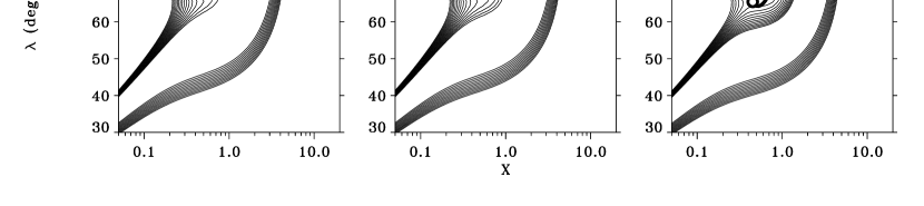
Figure 9: Isocontours of $g^{1-\alpha}/f$, normalized to $(2/3\sqrt{3})^{1-\alpha}$; from 0.855 to 0.885 in steps of $2\times 10^{-3}$ at the low saddle; from 1.05 to 1.15 in steps of $10^{-2}$ at the high saddle. At $r_{0}=4$, 4.03, and $4.15\,r_{\rm wd}$ (left to right panel). Heavy lines are solutions to the regularity condition. Circles mark the critical wind solution of maximum mass loss rate. Within the footpoint range from $r_{0}=4$ to $4.15\,r_{\rm wd}$, the wind switches from $\lambda_{\rm c}=80\arcdeg$ to $\lambda_{\rm c}=65\arcdeg$ via a growing regularity curve of ellipsoidal shape.

In order to fully understand the geometry of disk LDWs, we consider also the transition region between the inner and outer winds. As discussed above, the low saddle does not exist below $r_{0}\lesssim 4\,r_{\rm wd}$. Fig. 9 shows $g^{1-\alpha}/f$ in the neighborhood of this footpoint radius. At $r_{0}=4\,r_{\rm wd}$, only the high saddle exists and determines the wind solution. At $r_{0}=4.03\,r_{\rm wd}$, an inner regularity curve of elliptical shape has formed, but not yet the low saddle point of $g^{1-\alpha}/f$. The mass loss rate is maximal at the smallest $\lambda$ along the curve, i.e., at its lower tip, which determines the wind solution in this transition regime. Finally, by $r_{0}=4.15\,r_{\rm wd}$, a low saddle has formed at $\lambda_{\rm c}=65\arcdeg$. The wind tilt stays at this value $\lambda_{\rm c}$, which corresponds to the maximum mass loss rate. In total, the wind tilt switches continuously from the high to the low saddle over a narrow range of $0.1\,r_{\rm wd}$ in the footpoint radius.

5.4 Overall disk wind geometry

Table 1 lists important parameters of the wind above SHS and Newtonian disks, i.e., the tilt angle, $\lambda$, the normalized mass loss rate from a disk annulus, $\dot{m}$, and the critical point location, $X_{\rm c}$. The mass loss rate $\dot{m}$ is normalized to a vertical wind above an isothermal disk. The shallow maxima of the function ${\tilde{F}}_{x}$ in Fig. 5 are responsible for $\dot{m}=O(1)$. Implications of these mass loss rates are discussed in Paper II. From the table, one finds the ray dispersion in the outer wind, at intermediate footpoint radii from 4 to $10\,r_{\rm wd}$,

$${d\lambda\over dr_{0}}\simeq-{1\arcdeg\over\,r_{\rm wd}}.$$ (24)

Further in or out the ray dispersion is even smaller. Actually, since $d\lambda/dr_{0}$ enters the Euler equation (20), the full wind problem can be solved only iteratively. However, the dependence of the eigenvalues $E_{\rm c}$ and $\lambda_{\rm c}$ on $d\lambda/dr_{0}$ is weak, and we assume throughout that eq. (24) holds.

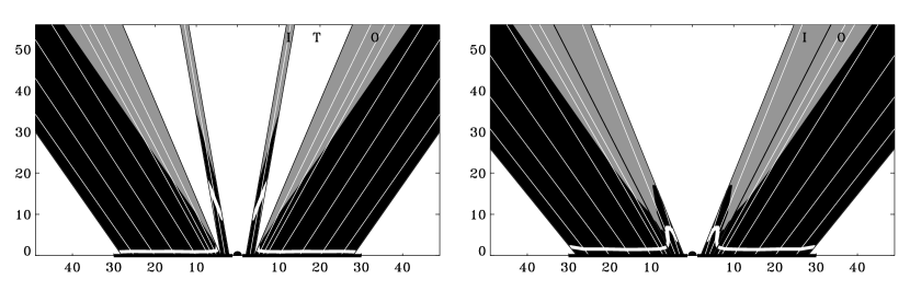
Figure 10: Wind geometry above the SHS disk ($r_{\rm d}=30\,r_{\rm wd}$) according to Table 1, for $\alpha=2/3$ (left panel) and 1/2 (right panel). Black regions indicate the accelerating LDW, and thin white lines show a few wind cones. Grey areas indicate decelerating wind (Appendix B), for a ray dispersion $d\lambda/dr_{0}=-1\arcdeg/\,r_{\rm wd}$. ‘I’ and ‘O’ mark the inner and outer wind, ‘T’ is the transition region. Heavy, white lines are locations of flow critical points. The innermost region of the disk, at $r_{0}<2\,r_{\rm wd}$, is not treated due to uncertainties in the radiation field.

The overall geometry of the disk wind is shown in Fig. 10. For $\alpha=2/3$, the critical points are at $x_{\rm c}\sim 10-20\,r_{\rm wd}$ for the inner wind, then move towards the disk photosphere and stay at $x_{\rm c}\simeq\,r_{\rm wd}$, independent of footpoint radius $r_{0}$ in the outer wind. For $\alpha=1/2$, on the other hand, the critical points lie somewhat higher for the outer wind, at $x_{\rm c}\simeq 2\,r_{\rm wd}$, but again independent of radius. While the division between the inner and outer wind persists (namely high-lying vs. low-lying saddle, or critical points on opposing sides of the gravity hill), the transition in $\lambda$ between the two regions is smooth for $\alpha=1/2$, and the inner tilt reaches a maximum of $\lambda=70\arcdeg$.

The innermost disk region, $1-2\,r_{\rm wd}$, is left out in Fig. 10. The details of the disk wind and its very existence here are subject to great uncertainties in the radiation field which depends on the properties of the transition layer and the white dwarf itself. The outer boundary of the disk LDW is set by the radius where the disk temperature falls below $10^{4}$ K and the wind driving becomes inefficient, in analogy with stellar winds (Abbott 1982; Kudritzki et al. 1998). For the SHS disk with $L_{\rm d}=10\,{\rm L}_{\odot}$, this should happen around $30\,r_{\rm wd}$.

6 Discussion

We compare here our theoretical model of LDWs from accretion disks in CVs with those available in the literature, kinematical and dynamical ones. We ignore the radial wind models, with the white dwarf being the wind base, because they are in a clear contradiction with current observations (e.g., review by Mauche & Raymond 1997). An alternative source of gas is the disk itself. Kinematical models which account for this source of material subject to the line-driving force successfully explained the observed bipolarity of the outflow, and reproduced the inclination-dependent line profiles (Shlosman & Vitello 1993). Their weak point was the absence of a unique solution. The 1-D dynamical models in a simplified disk radiation field revealed some major differences between the stellar and disk winds, e.g., the bi-polarity and the existence of a gravity hill (Vitello & Shlosman 1988).

More sophisticated 2-D kinematical models, supplemented with a 3-D radiation transfer in Sobolev approximation, showed the importance of rotation in shaping the lines (Vitello & Shlosman 1993; Shlosman et al. 1996). Finally, the 2-D hydrodynamical model of a disk wind in a realistic radiation field and with the line-force parameterized by the CAK approximation has addressed the issue of flow streamlines and mass loss rates in the wind (PSD). Our comparison, therefore, is focused on these models.

Vitello & Shlosman (1993) set up a kinematical disk wind model assuming straight flow lines in order to fit the C iv P Cygni line profiles of three CVs observed with the IUE. The fit parameters included the inner and outer terminating radius of the wind base, and the corresponding tilt angles of the wind cone. The best fit appeared to be indifferent to the mass loss rate, within the range of $10^{-1}$ to $10^{-2}$ of the accretion rate. In the present work, which accounts for wind dynamics, we find lower mass loss rates more justified and discuss various implications of these rates on the wind models in Paper II. The tilt of the innermost wind cone in Vitello & Shlosman was rather steep, $\lambda=80\arcdeg$, while at the outer disk edge $\lambda=25\arcdeg$. A similar work by Knigge et al. (1995), but using Monte Carlo radiation transfer in the wind, gave similar results. In the present work, the tilt angle $\lambda$ is calculated self-consistently from the Euler equation, resulting in a similar inner tilt as found from kinematical models, while the outer tilt differs by a factor of 2 between the two approaches.

The most advanced numerical modeling of CV winds from the SHS disk so far was performed by PSD, using the time-dependent Zeuss 2-D code. We find a number of similarities between their and our results, but differences exist as well. Our comparison with PSD is limited to their models 2–5, i.e., without a central luminous star. These models agree with ours on the overall wind geometry. This includes the streamline shapes and the run of the wind opening angle with height. The streamlines in PSD appear to form straight lines in the $(r,z)$ plane, in striking similarity with the previous kinematical models. In addition, the change in the wind opening angle with distance from the rotation axis seems to be weak in PSD. The mass loss rates are consistent between both models, and so are the wind optical depths, which can approach unity even for very strong resonance lines (Paper II).

While PSD also find two markedly distinct flow regions, the inner and outer, their inner wind, at $r_{0}\lesssim 4\,r_{\rm wd}$, appears as the sole and only outflow. The outer disk region, at radii $\gtrsim 4\,r_{\rm wd}$, exhibits a time-dependent irregular flow, resulting in no mass loss. In contrast, in our model, mass loss from the SHS disk is dominated by the inner wind and the innermost part of the outer wind, as is discussed in Paper II. Interestingly, our outer wind seems to be more robust than the inner wind. For the latter, the balance of driving and drag forces which leads to a high saddle on the far side of the gravity hill is rather a delicate one. Setting, for example, the centrifugal force arbitrarily to zero causes the high saddle solution to vanish, whereas the low saddle remains almost unchanged.

PSD suggest that the irregular behavior of the outer flow is a consequence of the different $X$-dependence of gravity and disk flux, with the gravity preventing the wind from developing. We find instead that at radii $r_{0}\gtrsim 4\,r_{\rm wd}$, where a low saddle exists, the fast increase in the projected disk flux, ${\tilde{F}}_{x}(X)$, results in a sufficiently strong growth of the line force which drives the wind past the gravity hill. For the inner wind regions, on the other hand, where no lower saddle branch exists, the wind indeed must overcome the gravity barrier without the appropriate radiation flux increase with $X$.

Based on our analysis of the disk wind we may provide some insight into the erratic behavior of the flow PSD observe at larger radii. It is possible that mass overloading of the flow causes spatial and temporal fluctuations of the streamline divergence $d\lambda/dr_{0}$, wherefore the wind stalls on characteristic length scales of the vertical gravity, $r_{0}$. We conjecture that fluctuations on such scales may be self-amplifying, or, in other words, result in a locally converging flow with $d\lambda/dr_{0}>0$. However, if such an instability exists, it is expected to be most pronounced in the inner disk regions. Namely, with increasing $r_{0}$, the flux increases faster with $X$, which moves the critical point closer to the sonic point. Mass overloading seems therefore less likely in the outer wind regions, in contrast to the findings of PSD. A linear stability analysis of our stationary wind model with respect to harmonic perturbations of $d\lambda/dr_{0}$ would also be interesting, but is beyond the scope of the present work.

Furthermore, we cannot confirm the dependence of $\lambda$ on the disk luminosity as in the PSD model. We find that the eigenvalue $\lambda_{\rm c}$ for each streamline is determined from the positions of the saddle points of the function $g^{1-\alpha}/f$. Both $g$ and $f$ are independent of the disk luminosity, $f$ specifically so because it is normalized to the flux at the streamline footpoint (eq. 21). Therefore, $\lambda_{\rm c}$ depends only on the radial temperature stratification in the disk.

One important issue neglected in our modeling is the saturation of the line force at some value when all the driving lines become optically thin. If this thick-to-thin transition occurs before the flow reaches its critical point, the wind solution is lost, since the drag forces overcome the driving forces. However, this still leaves the possibility that a more complicated wind dynamics is established, where the decelerating flow at some larger radius starts again to accelerate (i.e., jumps from a $W^{\prime}_{-}$ to a $W^{\prime}_{+}$ solution). We leave this question open for future scrutiny, and note here that the mass loss rates derived from the present eigenvalues $E$ are upper limits.

The present work is based on the CAK theory for stellar winds. Over the years, questions have been raised concerning the physical meaning of the CAK critical point (Thomas 1973; Lucy 1975; Cannon & Thomas 1977; Abbott 1980; Owocki & Rybicki 1986; Poe, Owocki, & Castor 1990). Most interesting for the present context is the inclusion of higher order corrections to the diffuse line force in the Sobolev approximation, which shift the critical point still closer to the sonic point (Owocki & Puls 1998; see also Fig. 1). This proximity of the sonic and critical points may not be coincidental, and one can speculate whether or not the sonic point determines the mass loss rate instead of the critical point. However, we find for the disk wind model that the sonic and critical points occasionally lie far apart, e.g., for a vertical wind above an isothermal disk, or a tilted wind close to the rotation axis (‘inner wind’).

These fundamental issues impair our understanding of LDWs from stars and disks, and therefore must be addressed in the future.

7 Summary

We discuss an analytical model for 2-D stationary winds from accretion disks in cataclysmic variable stars. All parameters chosen are typical for high-accretion rate disks in novalike CVs. We solve the Euler equation for the wind, accounting for a realistic radiation field above the disk, which drives the wind by means of radiation pressure in spectral lines. Some key assumptions are that each helical streamline lies on a straight cone; that the driving line force can be parameterized according to CAK theory; and that the thermal gas pressure in the supersonic wind can be neglected. Our results can be summarized as follows.

The disk wind solutions are characterized by two eigenvalues, the mass loss rate and the flow tilt angle, $\lambda_{\rm c}$, with the disk. The additional eigenvalue $\lambda_{\rm c}$ for each streamline reflects the 2-D nature of the model. We find that the wind exhibits a clear bi-conical geometry with a small ray dispersion. Specifically, two regions, inner and outer, can be distinguished in the wind, launched from within and outside $4\,r_{\rm wd}$, respectively. The tilt angle for the outer wind is $\lambda\sim 60\arcdeg$ with the disk. At these angles, the wind flow and radiative disk flux are well aligned. For the inner wind, the tilt angle is larger, up to $80\arcdeg$. We emphasize that the disk wind tilt angle (i.e., the wind collimation) depends solely upon the radial temperature stratification in the disk, unless there is an additional degree of freedom such as central luminosity associated with nuclear burning on the surface of the white dwarf.

A major distinction between stellar and disk winds is the existence of maxima in both the gravity and the disk flux along each streamline. The latter flux maximum appears to be a crucial factor in allowing the wind to pass over the gravity ‘hill’. The flux increase is more pronounced further away from the rotation axis. As a result, the critical point of the outer wind lies close to the disk photosphere and to the sonic point. In fact, it lies upstream of the top of the gravity hill, and this proximity of the critical and sonic points is typical of LDWs from O stars as well. On the other hand, for the inner wind, the increase in radiation flux with height is smaller, and the critical point lies far away from the sonic point, beyond the gravity hill.

Comparing our analytical models with the 2-D numerical simulations of Proga et al. (1998), we find an overall good agreement in the streamline shape, tilt angle, and mass loss rate, but our wind baseline is wider.

Appendix A Line force due to gradients in the azimuthal velocity

We estimate here the importance of azimuthal velocity terms for the line force in $x$-direction. Assuming Keplerian rotation within the disk, and angular momentum conservation above the disk, one has

$${\displaystyle\partial v_{\phi}/\partial z\over\displaystyle\partial v_{x}/\partial x} = -{\displaystyle 1\over\displaystyle\sqrt{2}}\;{\displaystyle 1\over\displaystyle\tan\lambda}\;{\displaystyle 1\over\displaystyle 1+X\cos\lambda}\;{\displaystyle\sqrt{W}\over\;\displaystyle W^{\prime}},$$

$${\displaystyle\partial v_{\phi}/\partial r\over\displaystyle\partial v_{x}/\partial x} = -{\displaystyle 1\over\displaystyle\sqrt{2}}\;{\displaystyle 1-X\cos\lambda\over\displaystyle(1+X\cos\lambda)^{2}}\;{\displaystyle\sqrt{W}\over\;\displaystyle W^{\prime}},$$ (A1)

$$-{\displaystyle v_{\phi}/r\over\displaystyle\partial v_{x}/\partial x} = -{\displaystyle\sqrt{2}\over\displaystyle(1+X\cos\lambda)^{2}}\;{\displaystyle\sqrt{W}\over\;\displaystyle W^{\prime}}.$$

Here, the singularity of $\tan^{-1}\lambda$ at $\lambda=0$ is a result of neglecting the pressure terms in the Euler equation. Note that $\partial v_{\phi}/\partial r$ changes sign at $X=1/\cos\lambda$. From (A), gradients in $v_{\phi}$ are comparable to gradients in $v_{x}$ when $\sqrt{W}/W^{\prime}\sim 1$. The main question is for their influence on the mass loss rate. Because, in the CAK model, $\dot{M}$ is determined by the conditions at the critical point, we calculate $\sqrt{W}/W^{\prime}$ at the latter. We consider first a vertical wind from an isothermal disk. Since $W^{\prime}$ grows monotonically up to and somewhat beyond the critical point (see Fig. 8), and because $W=\int W^{\prime}dX$, one has $\sqrt{W_{\rm c}}/W^{\prime}_{\rm c}<$ $(3/2)^{3/4}\sqrt{1-\alpha/\alpha}\sim 1$. Here, $X_{\rm c}=1/\sqrt{2}$ and eq. (18a) were used. Alternatively, the critical points of the outer wind above a non-isothermal disk typically lie close to the disk, hence $g(X)\simeq X$. Using eq. (22a), $\sqrt{X_{\rm c}/W^{\prime}_{\rm c}}\sim\sqrt{1-\alpha/\alpha}\sim 1$. Both disk cases give, therefore, essentially the same result. We conclude that $v_{\phi}$-terms can be important everywhere between the disk photosphere and the critical point, and hence can modify $\dot{M}$.

To find their effect on $\dot{M}$, we include $v_{\phi}$-terms in the evaluation of the line force, eq. (2), in an approximate manner. Only the disk regime is considered, in which case the radiation intensity is roughly isotropic and the radiation flux has a $z$-component only. The azimuthal part of the solid angle integral in (2) is approximated by a 4-point quadrature at angles $n\pi/2$ with ${\bf\hat{r}}$, where $n=0,1,2,3$. This leads to a correction factor of the approximate form ${1\over 4}\bigl{(}2+|1+S|^{\alpha}+|1-S|^{\alpha}\bigr{)}$ to the line force, $EfW^{\prime\alpha}$. Here, $S$ is a linear combination of the expressions in eq. (A), with coefficients $<1$ from angle integration. In the disk regime, $S_{\rm c}\sim 1$ from eq. (A). This coincides with the borderline between an increase and a decrease in $\dot{M}$ due to inclusion of $v_{\phi}$-terms, which lies at $S_{\rm c}=1.25$ for $\alpha=1/2$ and at $S_{\rm c}=1.18$ for $\alpha=2/3$. A detailed, numerical calculation of the above angle integral is required to decide, which of both cases actually occurs. Since, however, $S_{\rm c}$ is close to unity, the influence on the mass loss rate is limited to a 10% effect. We, therefore, neglect $v_{\phi}$-terms in calculating the line force.

Appendix B Disk wind deceleration

In Figure 6, isocontours which cross through the low saddle point loop into one another at some larger height, $X_{\rm d}$. At $X>X_{\rm d}$, one has $E>E_{\rm c}$ from the figure, i.e., the allowed maximum mass loss rate in this region is smaller than that at the saddle. At these distances, inertia and gravity overcome the line force plus centrifugal force, and the wind decelerates, $W^{\prime}<0$. As is shown in Paper II, the wind speed always exceeds the local escape speed at $X_{\rm d}$, which implies that the decelerating wind reaches infinity at a positive speed.

Due to the deceleration, the velocity law becomes non-monotonic, and the line transfer is no longer purely local, because global couplings occur between distant resonance locations. We neglect these couplings here, and simply replace $W^{\prime\alpha}$ in the line force by $|W^{\prime}|^{\alpha}$. For a wind ray launched at $r_{0}=5\,r_{\rm wd}$, Fig. 8 shows that a single, decelerating branch, $W^{\prime}_{-}<0$, accompanies the critical, accelerating solution $W^{\prime}_{+}$ of maximum mass loss rate. It is suggestive that at $X_{\rm d}$ the solution curve jumps from the $W^{\prime}_{+}$ to the $W^{\prime}_{-}$ branch, and extends thereupon to infinity.

The discontinuity in $W^{\prime}$ introduces a kink in the velocity law. Such kinks propagate at sound speed (Courant & Friedrichs 1948; actually, for LDWs, at some modified, radiative-acoustic speed, see Abbott 1980 and Cranmer & Owocki 1996) and are therefore inconsistent with the assumption of stationarity. It seems plausible, however, that the discontinuity in $W^{\prime}$ is an artifact of the Sobolev approximation, since the latter becomes invalid at small $dv/dx$, i.e., as $W^{\prime}\rightarrow 0$. An exact line transfer should instead give a smooth transition from $W^{\prime}_{+}$ to $W^{\prime}_{-}$. We find indeed cases of ‘almost’ smooth transitions, where both $dW^{\prime}_{+,-}/dX_{\rm d}\rightarrow-\infty$, e.g., in the top panel of Fig. 8.

Table 1: Tilt angle $\lambda_{\rm c}$, normalized mass loss rate $\dot{m}_{\rm c}$, and position $X_{\rm c}$ of the critical point for different disk wind models. Underlined numbers indicate the transition from the inner to the outer wind.

	SHS Disk						Newtonian Disk
	$\alpha=2/3$			$\alpha=1/2$			$\alpha=2/3$			$\alpha=1/2$
$r_{0}/r_{\rm wd}$	$\lambda_{\rm c}[\arcdeg]$	$\dot{m}_{\rm c}$	$X_{\rm c}$	$\lambda_{\rm c}$	$\dot{m}_{\rm c}$	$X_{\rm c}$	$\lambda_{\rm c}$	$\dot{m}_{\rm c}$	$X_{\rm c}$	$\lambda_{\rm c}$	$\dot{m}_{\rm c}$	$X_{\rm c}$
2	80	0.42	4.4	68	0.62	1.9	78	0.64	4.3	65	0.94	1.2
3	80	0.60	4.4	72	1.02	2.3	78	0.90	4.7	65	1.45	0.82
4	80	0.86	4.4	69	1.60	1.7	65	1.23	0.32	63	1.78	0.58
5	64	1.37	0.26	63	2.23	0.52	64	1.32	0.26	62	2.10	0.43
6	62	1.48	0.19	61	2.69	0.35	63	1.37	0.23	61	2.23	0.38
7	61	1.60	0.16	60	3.08	0.27	63	1.37	0.21	61	2.37	0.34
10	58	1.82	0.11	58	3.84	0.18	62	1.48	0.17	60	2.69	0.28
15	57	2.10	0.08	55	5.41	0.12	61	1.54	0.15	58	3.08	0.23
20	56	2.26	0.06	53	6.57	0.10	60	1.60	0.13	58	3.31	0.2
25	55	2.45	0.05	52	8.16	0.08	60	1.67	0.13	57	3.31	0.3
28	55	2.59	0.04	51	8.16	0.10	58	1.35	0.2	57	2.44	0.2

Figure 1: Saddle point topology of stellar CAK winds in the $(W^{\prime},U)$ plane, for (a) a point star and zero sound speed; (b) a point star and finite sound speed; (c) an extended star and finite sound speed. Filled dots mark the sonic points (at $U\simeq-1$) and the critical points.

Figure 2: Adopted flow geometry for a CV disk wind. The streamlines are helical lines, and are assumed to lie on straight cones.

Figure 3: Isocontours of the frequency-integrated, vertical flux component $F_{z}$ above a Newtonian disk. The disk extends from 1 to $30\,r_{\rm wd}$. Normalization is $I(r_{0}=5\,r_{\rm wd},z=0)=1$.

Figure 4: Same as Fig. 3, including normalization, here for the radial flux component $F_{r}$. Dotted lines indicate an inward flux.

Figure 5: Normalized, projected flux ${\tilde{F}}_{x}(r_{0},X)$ for SHS (top panel) and Newtonian (bottom panel) disks, at footpoint radii $r_{0}=20$, 10, 5, and $2\,r_{\rm wd}$ (top to bottom curves). The tilt angle with the disk plane is $90\arcdeg$ (full lines) and $60\arcdeg$ (dashed lines).

Figure 6: Isocontours of $g^{1-\alpha}/f$, normalized to $(2/3\sqrt{3})^{1-\alpha}$, over the $(X,\lambda)$ plane. Footpoints of the wind are at $r_{0}=3$, 5, and $15\,r_{\rm wd}$ (left to right panel). The isocontours have logarithmic spacing. The temperature stratification is that of the SHS disk ($r_{\rm d}=30\,r_{\rm wd}$, $\alpha=2/3$). Heavy lines are solutions to the regularity condition (22c).

Figure 7: Radiative flux vector above the SHS disk ($r_{\rm d}=30\,r_{\rm wd}$). The straight line indicates a wind cone at eigenvalue $\lambda=61\arcdeg$ (cf. Table 1). The ‘$+$’ sign marks the critical point.

Figure 8: Critical wind solutions $W^{\prime}(X)$ at zero sound speed, above the SHS disk ($r_{\rm d}=30\,r_{\rm wd}$, $\alpha=2/3$). At $r_{0}=3\,r_{\rm wd}$: high saddle; at $r_{0}=5$ and $15\,r_{\rm wd}$: low saddle. The branches $W^{\prime}<0$ are decelerating wind solutions, and are discussed in Appendix B. ‘$+$’ and ‘$-$’ signs refer to the sign of the Euler function $P$ in eq. (20). For comparison with the critical point topology of a spherically symmetric, stellar wind, see Fig. 1.

References

- (1)
- (2) Abbott, D. C. 1980, ApJ, 242, 1183
- (3) Abbott, D. C. 1982, ApJ, 259, 282
- (4) Arav, N., Shlosman, I., & Weymann, R. J. (eds.) 1997, ASP Conf. Series 128, Mass Ejection from Active Galactic Nuclei (San Francisco: ASP)
- (5) Begelman, M. C., McKee, C. F., & Shields, G. A. 1983, ApJ, 271, 70
- (6) Binney, J., & Tremaine, S. 1987, Galactic Dynamics (Princeton: University Press), 664
- (7) Bjorkman, J. E. 1995, ApJ, 453, 369
- (8) Blandford, R. D., & Payne D. G. 1982, MNRAS, 199, 883
- (9) Cannon, C. J., & Thomas, R. N. 1977, ApJ, 211, 910
- (10) Cassinelli, J. P. 1979, ARA&A, 17, 275
- (11) Castor, J. I. 1974, MNRAS, 169, 279
- (12) Castor, J. I., Abbott, D. C., & Klein R. I. 1975, ApJ 195, 157 (CAK)
- (13) Córdova, F. A., & Mason, K. O. 1982, ApJ, 260, 716
- (14) Córdova, F. A., & Mason, K. O. 1985, ApJ, 290, 671
- (15) Courant, R., & Friedrichs, K. O. 1948, Supersonic Flow and Shock Waves (New York: Interscience Publishers)
- (16) Cranmer, S. R., & Owocki, S. P. 1996, ApJ, 462, 469
- (17) Diaz, M. P., Wade, R. A., & Hubeny, I. 1996, ApJ, 459, 236
- (18) Emmering, R. T., Blandford, R. D., & Shlosman, I. 1992, ApJ, 385, 460
- (19) Feldmeier, A., Shlosman, I., & Vitello, P. 1999, ApJ, submitted (Paper II)
- (20) Gayley, K. G., Owocki, S. P., & Cranmer, S. R. 1999, ApJ, submitted
- (21) Heap, S. R., et al. 1978, Nature, 275, 385
- (22) Holzer, T. E. 1977, J. Geophys. Res., 82, 23
- (23) Horne, K., & Cook, M. C. 1985, MNRAS, 214, 307
- (24) Horne, K., & Stiening, R. F. 1985, MNRAS, 216, 933
- (25) Icke, V. 1980, AJ, 85, 329
- (26) Klare, G., Wolf, B., Stahl, O., Krautter, J., Vogt, N., Wargau, W., Rahe, J. 1982, A&A, 113, 76
- (27) Knigge, C., Woods, J. A., & Drew, J. E. 1995, MNRAS, 273, 225
- (28) Krautter, J., Vogt, N., Klare, G., Wolf, B., Duerbeck, H. W., Rahe, J., Wargau, W. 1981, A&A, 102, 337
- (29) Kudritzki, R. P., Springmann, U., Puls, J., Pauldrach, A., & Lennon, M. 1998, ASP Conf. Series 131, Boulder-Munich II: Properties of Hot, Luminous Stars, ed. I. Howarth (San Francisco: ASP), 278
- (30) Lamers, H., & Cassinelli J. P. 1999, Introduction to Stellar Winds (Cambridge: University Press)
- (31) Livio, M. 1997, ASP Conf. Series 121, Accretion Phenomena and Related Outflows, ed. D. T. Wickramasinghe, G. V. Bicknell, L. Ferrario (San Francisco: ASP), 8
- (32) Lucy, L. B. 1975, Memoires Societe Royale des Sciences de Liege, 8, 359
- (33) Lucy, L. B., & Solomon, P. M. 1970, ApJ, 159, 879
- (34) Mauche, C. W., & Raymond J. C. 1997, Cosmic Winds and the Heliosphere, ed. J. R. Jokipii, C. P. Sonett, & M. S. Giampapa (Tucson: Univ. of Arizona Press), 111
- (35) Mauche, C. W., et al. 1999, ApJ, in preparation
- (36) Mihalas, D., & Mihalas B. 1984, Foundations of Radiation Hydrodynamics (New York: Oxford University Press)
- (37) Murray, N., & Chiang, J. 1996, Nature, 382, 789
- (38) Owocki, S. P., Castor, J. I., & Rybicki, G. B. 1988, ApJ, 335, 914
- (39) Owocki, S. P., & Puls, J. 1996, ApJ, 462, 894
- (40) Owocki, S. P., & Puls, J. 1998, ApJ, 510, 355
- (41) Owocki, S. P., & Rybicki, G. B., 1984 284, 337
- (42) Owocki, S. P., & Rybicki, G. B., 1985 299, 265
- (43) Owocki, S. P., & Rybicki, G. B., 1986 309, 127
- (44) Pauldrach, A. 1987, A&A, 183, 295
- (45) Pauldrach, A., Kudritzki, R. P., Puls, J., Butler, K., & Hunsinger, J. 1994, A&A, 283, 525
- (46) Pauldrach, A., Puls, J., & Kudritzki, R. P. 1986, A&A, 164, 86
- (47) Pereyra, N. A., Kallman, T. R., & Blondin, J. M. 1997, ApJ, 477, 368
- (48) Poe, C. H., Owocki, S. P., & Castor, J. I. 1990, ApJ, 358, 199
- (49) Proga, D., Stone, J. M., & Drew, J. E. 1998, MNRAS, 295, 595 (PSD)
- (50) Pudritz, R. E., & Norman, C. A. 1986, ApJ, 301, 571
- (51) Puls, J., Springmann, U., & Lennon, M. 1999, A&A, submitted
- (52) Puls, J., Springmann, U., & Owocki, S. P. 1998, Cyclical Variability in Stellar Winds, ed. L. Kaper, & A. W. Fullerton (Berlin: Springer), 389
- (53) Rutten, R. G., Dhillon, V. S., Horne, K., Kuulkers, E., & Van Paradijs, J. 1993, Nature, 362, 518
- (54) Shakura, N. I., & Sunyaev, R. A. 1973, A&A, 24, 337 (SHS)
- (55) Shlosman, I., & Vitello, P. 1993, ApJ, 409, 372
- (56) Shlosman, I., Vitello, P., & Mauche C. W. 1996, ApJ, 461, 377
- (57) Shlosman, I., Vitello, P., & Shaviv, G. 1985, ApJ, 294, 96
- (58) Sobolev, V. V. 1957, Soviet Astr., 1, 678
- (59) Thomas, R. N. 1973, A&A, 29, 297
- (60) Vitello, P., & Shlosman, I. 1988, ApJ, 327, 680
- (61) Vitello, P., & Shlosman, I. 1993, ApJ, 410, 815
- (62) Woods, D. T., Klein, R. I., Castor, J. I., McKee, C. F., & Bell, J. B. 1996, ApJ, 461, 767
- (63)