Excitation of warps by spiral waves in galaxies by non-linear coupling

Abstract

We present a new mechanism to explain the frequently observed and thus certainly permanent warping of spiral galaxies. We consider the possibility of non-linear coupling between the spiral wave of the galaxy and two warp waves, such that the former, which is linearly unstable and extracts energy and angular momentum from the inner regions of the galactic disk, can continuously feed the latter. We derive an expression for the coupling coefficient in the WKB approximation. We show that the coupling is too weak in the stellar disk, except at the Outer Lindblad Resonance where the spiral slows down and is efficiently coupled to warp waves. There, the spiral can be almost completely converted into “transmitted” warps, which we can observe in HI, and a “reflected” one, which we can observe as a corrugation. Our mechanism reproduces the observed amplitudes of the warp and of the corrugation, and might explain related phenomena such as the behavior of the line of nodes of the warp. Furthermore we show that the energy and momentum fluxes of observed spirals and warps are of the same order of magnitude, adding a strong point in favor of this model.

1 Introduction

Spiral galaxies often show a warping of their external parts, observed in HI. Such warps appear like an “S” or an integral sign for galaxies observed edge-on (Sancisi, 1976).

This phenomenon, known since 1957, has led to theoretical difficulties. Warps are bending waves, and we correctly understand their propagation (see Hunter, 1969a for a dispersion relation in an infinitely thin disk, and see Nelson 1976a and 1976b, Papaloizou and Lin 1995, Masset and Tagger 1995 for the dispersion relation taking into account finite thickness and compressional effects), but we do not know the mechanism responsible for their excitation. It cannot be systematically justified by tidal effects (Hunter and Toomre 1969), since we observe warping of very isolated spiral galaxies. It cannot be explained by a temporary excitation, since a warp propagates radially in the disk is not reflected at its edge, so that it should disappear over a few galactic years (Hunter, 1969b). Attempts have been made to connect the existence of warps and the properties of haloes (Sparke, 1984a, Sparke and Casertano 1988, Hofner and Sparke 1994). The mechanism proposed by Sparke and Casertano (1988) implies an ad hoc misalignment angle between the normal axis of the galactic plane and the “polar” axis of the halo. This mechanism has recently encountered self-consistency difficulties (Dubinski and Kuijken 1995). Furthermore, it relies on the dubious hypothesis of a rigid and unresponsive halo. Several explanations have also been proposed, such as the infall of primordial matter (Binney, 1992), the effect of the dynamical pressure of the intergalactic medium, etc…. For a review of all the proposed mechanisms, see Binney (1992).

Binney (1978, 1981) has considered the possibility of a resonant coupling between the vertical motion of a star and the variation of the galactocentric force, due to a halo or a bar. He concluded that a bar could be responsible for the observed warps and corrugations. Sparke (1984b) has also explored this possibility, and considered the growth of a warp from a bar or a triaxial halo. She found that a bar was unlikely to be responsible for a warp, but she emphasized that a triaxial halo could quite well reproduce observed warps.

We consider here another mechanism, the non-linear coupling between a spiral wave and two warp waves. Non-linear coupling between spirals and bars has already been found (Tagger et al. 1987 and Sygnet et al. 1988) to provide a convincing explanation for certain behaviors observed in numerical simulations (Sellwood 1985), or observed in Fourier Transforms of pictures of face-on galaxies. The relative amplitude of spiral or warp waves (the ratio of the perturbed potentials to the axisymmetric one) is about $\sim 0.1$ to $\sim 0.3$ (see Strom et al. 1976). Non-linear coupling involves terms of second order in the perturbed potential, while linear propagation is described by first order terms. Classically one would thus believe that non-linear coupling is weak at such small relative amplitudes. However in the above-mentioned works it was found that the presence of resonances could make the coupling much more efficient if the wave frequencies are such that their resonances (i.e. the corotation of one wave and a Lindblad resonance of another one) coincide. At this radius the non-linear terms become comparable with the linear ones, so that the waves can very efficiently exchange energy and angular momentum. Indeed in Sellwood’s (1985) simulations, as discussed by Tagger et al. (1987) and Sygnet et al. (1988), an “inner” spiral or bar wave, as it reaches its corotation radius, transfers the energy and angular momentum extracted from the inner parts of the disk to an “outer” one whose ILR lies at the same radius, and which will transfer them further out, and ultimately deposit them at its OLR. In this process the energy and momentum are thus transferred much farther radially than they would have been by a single wave, limited in its radial extent by the peaked rotation profile.

We will show here that a similar mechanism, now involving one spiral and two warp waves is not only possible (by the “selection rules” associated with their parity and wavenumbers), but also very efficient if the same coincidence of resonances occurs. This allows the spiral wave, as it reaches its OLR (and from linear theory deposits the energy and momentum extracted from the inner regions of the disk) to transfer them to the warps which will carry them further out.

Unlike Tagger et al. (1987) and Sygnet et al. (1988), we will throughout this paper restrict our analysis to gaseous rather than stellar disks, described from hydrodynamics rather than from the Vlasov equation. The reason is that our interest here lies mainly in the excitation of the warps, which propagate essentially in the gas (indeed the outer warp is observed in HI, and the corrugation is most likely (Florido et al. 1991) due to the motion of the gaseous component of the galactic disk). On the other hand, the spiral wave propagates in the stellar as well as the gaseous disk. The difference is important only in the immediate vicinity of Lindblad resonances, where the spiral wave is absorbed; as a consequence, its group velocity vanishes at the resonances. Since the group velocity of the waves will appear as an important parameter, we will choose to keep the analytic coupling coefficient derived from the hydrodynamic analysis, but we will introduce, for the spiral density wave, the group velocity of a stellar spiral. From the physics involved this will appear as a reasonable approximation; furthermore it should only underestimate the coupling efficiency, since it does not include the resonant stellar motions near the resonance.

On the other hand, we will show that non-linear coupling is efficient only in a narrow annulus close to the OLR of the spiral, over a scale length similar to the one of Landau damping. We will thus conclude that the two processes are in direct competition, with the spiral transferring its energy and momentum, in part to the stars by Landau damping, and in part to the warps which will transfer them further outward, the exact repartition between these mechanisms presumably depending on detailed characteristics of the galactic disk.

The paper is organized as follows: in a first part we will introduce the notations, and the selection rules relative to the coupling. In a second part, we will derive the coupling coefficient from the hydrodynamic equations expanded to second order in the perturbed quantities, and we will try and simplify it. In a third part, we will analyze the efficiency of the coupling, together with the locations where it may occur. In the last sections we will compare our predictions to the observations, and we will propose some possible observational tests of our mechanism.

Some of the computations are tedious and lengthy. For the sake of clarity, they are developed in appendices, so as to retain in the main text only the principal results and the physical discussions.

2 Formalism and selection rules

2.1 Notations

We develop all our computations in the well-known shearing sheet approximation, which consists in rectifying a narrow annulus around the corotation radius of the spiral wave into a Cartesian slab. The results given by an exact computation taking into account the cylindrical geometry of the galaxy would differ by some metric coefficients, but would not differ physically from the shearing sheet predictions, so that the main conclusions would remain valid. We call $x$ the radial coordinate, with its origin at the corotation of the spiral, and oriented outward. We call $y$ the azimuthal coordinate, oriented in the direction of the rotation, and $z$ the vertical one, so as to construct a right-oriented frame $xyz$.

The hydrodynamic quantities are the density $\rho$, the speed components $(U,V,W)$, and the gravitational potential $\phi$. We assume that the disk is isothermal, with a uniform temperature, in order to avoid unnecessary complexity. Thus we can write: $P=a^{2}\rho$, where $P$ is the pressure and $a$ the isothermal sound speed.

The perturbed quantities are denoted with subscripts $1$, $2$ or $S$ referring to the wave involved (one of the two warps or the spiral wave), and equilibrium quantities with a subscript $0$.

The epicyclic frequency is denoted by $\kappa$, the rotation frequency by $\Omega$, Oort’s first constant by $A=\Omega^{\prime}r/2$, and we have the relation:

$$\kappa^{2}=4\Omega(\Omega+A)$$

We call $\mu$ the vertical characteristic frequency of the disk. We have:

$$\mu^{2}=2\Omega^{2}-\kappa^{2}$$

(see Hunter and Toomre, 1969). This frequency plays the same role for bending waves as $\kappa$ does for spiral waves; it should not be confused with the frequency $\nu_{z}$ of the vertical motion of individual particles, which is usually much higher. Indeed individual particles move vertically in the potential well of the disk, giving them the high frequency $\nu_{z}$. On the other hand, when one considers motions of the whole disk, the potential well moves together with the disk and exerts no restoring force. This leaves only a weaker restoring force, giving the vertical frequency $\mu$ as discussed e.g. in Hunter and Toomre (1969) or Masset and Tagger (1995).

For each of the three waves we consider, we denote by $\omega$ its frequency in the galactocentric frame, $m$ its azimuthal wavenumber ($m=2$ for a two-armed spiral, and $m=1$ for an “integral-sign” warp), $\tilde{\omega}=\omega-m\Omega(r)$ its frequency in a local frame rotating with the matter. In the peculiar case of the shearing sheet, we note $k_{y}=m/r$ where $r$ is the distance to the galactic center, and $k_{y}$ the azimuthal wavenumber.

We will have to perform part of our computations in the WKB approximation, i.e. assume that the radial wavevector varies relatively weakly over one radial wavelength; in practice, in the shearing sheet, this reduces to the classical “tightly wound” approximation, $k_{y}\ll k_{x}$. We will also use $q=\sqrt{k_{x}^{2}+k_{y}^{2}}$, the modulus of the “horizontal” wavevector. In the tightly wound approximation one has $q\simeq|k_{x}|$.

We also introduce $s=\rho/\rho_{0}$, and various integrated quantities:

$$\sigma=\int_{-\infty}^{+\infty}\rho(z)dz$$

the perturbed surface density,

$$\Sigma=\int_{-\infty}^{+\infty}\rho_{0}(z)dz$$

the equilibrium surface density, and:

$$Z=\frac{1}{\Sigma}\int_{-\infty}^{+\infty}z\rho(z)dz$$

the mean vertical deviation of a column of matter from the midplane, under the influence of a warp.

Figure 1: This figure summarizes our main notations relative to perturbed velocity and disk thickness.

We call $H$ the characteristic thickness of the disk. The vertical density profile in the disk is taken to be consistent (see Masset and Tagger, 1995), i.e. it must fulfill simultaneously the Poisson equation and the hydrostatic equilibrium equation, with the additional condition that the radial derivatives of the equilibrium potential do not depend on $z$ throughout the disk thickness: this condition results from the hypothesis of a disk which is geometrically thin, $H\ll r$, although we do resolve vertically the perturbed quantities along the vertical direction.

Figure 2: This figure summarizes our notations relative to waves (spiral or warps). The column of matter has a section unity. At equilibrium (or more generally without spiral wave) it contains a mass $\Sigma$, and when perturbed by a spiral wave it contains the mass $\Sigma+\sigma$.

We summarize most of our notations in figures 1 and 2 and in table 1.

Symbol	corresponding quantity
$a$	Sound speed
$\Omega$	Equilibrium angular velocity of matter
$A$	Oort’s first constant. $A=1/2rd\Omega/dr$
$\kappa$	Epicyclic frequency. $\kappa^{2}=4\Omega(\Omega+A)$
$\mu$	“Global vertical frequency”. $\mu^{2}=2\Omega^{2}-\kappa^{2}$
$\omega$	Wave frequency in galactocentric frame.
$\tilde{\omega}$	Wave frequency in rotating frame.
$\phi$	Perturbed potential.
$\rho$	Perturbed density.
$s$	Relative perturbed density ($s=\rho/\rho_{0}$).
$q$	Wave-vector modulus ($q=(k_{x}^{2}+k_{y}^{2})^{1/2}$)

Table 1: In this table we summarize the main frequencies of our system, and some other quantities related to warps or spirals.

2.2 Notion of coupling and selection rules

2.2.1 Mode coupling

As discussed in the introduction, we consider the coupling between a spiral wave and two warp waves. This coupling is necessarily a non-linear mechanism. In a linear analysis, each wave can be studied independently, by projecting perturbed quantities onto the frequency and the wavevector of each wave. In particular, combining the hydrodynamic (continuity and Euler) equations and the Poisson equation leads to the dispersion relation which reads, in the WKB limit:

$$\tilde{\omega}_{S}^{2}=\kappa^{2}-2\pi G\Sigma q_{S}+a^{2}q_{S}^{2}$$

for a spiral and:

$$\tilde{\omega}_{W}^{2}=\mu^{2}+2\pi G\Sigma q_{W}+\frac{\tilde{\omega}_{W}^{2}}{\tilde{\omega}_{W}^{2}-\kappa^{2}}a^{2}q_{W}^{2}$$

for a warp (see Masset and Tagger 1995, Papaloizou and Lin 1995).

Here we expand the hydrodynamic equations to second order in the perturbed quantities. Then the waves do not evolve independently anymore and, provided that they satisfy selection rules which will be discussed below, they can exchange energy and angular momentum.

Thus the problem we address can be described as follows:

We consider a spiral wave, with a given flux (its energy density multiplied by its group velocity), traveling outward, from its corotation to the Holmberg radius of the galaxy. We will not discuss here how this spiral has been excited and we do not try to justify its amplitude, but rather take it as an observational fact.

As it travels radially the spiral interacts with warps which are always present, at all frequencies, at a noise level associated with supernovae explosions, remote tidal excitations, etc.

Our goal is the following: can we find conditions such that, although the warps are initially at this low noise level, they can be non-linearly coupled to the spiral so efficiently that they absorb a sizable fraction of its energy and momentum flux ? And can these conditions be met commonly enough to explain the frequent (one might even say general) occurrence of warps and their main observational properties ?

We will first discuss the conditions, known as “selection rules”, for the warps to be coupled to the spiral.

2.2.2 Selection Rules

The linearized set of equations governing the wave behavior (continuity, Euler and Poisson) is homogeneous and even in $z$, so that any field of perturbations to the equilibrium state of the disk can be considered as composed of two independent parts:

• Perturbations whose perturbed density is even in $z$, and thus, due to hydrodynamic equations, whose perturbed quantities are all even in $z$ except $W$, which is odd. These perturbations are spiral waves, since they imply a perturbed density (a non-vanishing $\sigma$), and a vanishing $Z$ (so they do not raise the mid-plane of the disk).

• Perturbations whose perturbed density is odd in $z$, and thus whose perturbed quantities are all odd in $z$, except $W$, which is even. These perturbations are warps, since they imply a vanishing integrated perturbed density and a non-vanishing $Z$, which means that they involve a global motion of the mid-plane of the disk.

Furthermore, since the coefficients of the equations do not depend on time or azimuthal angle, Fourier analysis allows to separate solutions identified by their frequency and azimuthal wavenumber. On the other hand, since the coefficient do depend on the radius, Fourier analysis in $r$ (or $x$ in the shearing sheet) does not allow the definition of a radial wavenumber except in the WKB approximation. We will return to this below.

So let us consider a spiral wave for which we write:

$$\xi_{S}\propto e^{i(m_{S}\theta-\omega_{S}t)}$$

and two warp waves with:

$$\xi_{1}\propto e^{i(m_{1}\theta-\omega_{1}t)}$$

and

$$\xi_{2}\propto e^{i(m_{2}\theta-\omega_{2}t)}$$

where $\xi$ represents any perturbed quantity. Hydrodynamic equations written to second order in perturbed quantities will contain terms involving the products $\xi_{1}\xi_{2}$, $\xi_{1}\xi_{2}^{*}$, $\xi_{1}^{*}\xi_{2}$, etc.

Let us consider for instance the term $\xi_{1}\xi_{2}$ (rules for the other products are derived in a similar manner). Its behavior with time and azimuthal angle is:

$$\xi_{1}\xi_{2}\propto e^{i[(m_{1}+m_{2})\theta-(\omega_{1}+\omega_{2})t]}$$

More physically this product, which appears from such terms as $V_{1}.\nabla V_{2}$ or $\rho_{1}\nabla\phi_{2}$, can be interpreted as a beat wave. Fourier analysis in $t$ and $\theta$ will give a contribution from this term, at frequency $\omega_{1}+\omega_{2}$ and wavenumber $m_{1}+m_{2}$; thus it can interact with the spiral wave if:

$$\omega_{1}+\omega_{2}=\omega_{S}$$

and

$$m_{1}+m_{2}=m_{s}$$

As discussed above, the equations for the spiral wave are derived from the part of the perturbed quantities which is even in $z$. Our third selection rule is thus that the product $\xi_{1}\xi_{2}$ be even in $z$.

If we were in a radially homogeneous system, so that waves could also be separated by their radial wavenumber, a fourth selection rule would be:

$$k_{x1}+k_{x2}=k_{xS}.$$

Since this is not the case, we will write a coupling coefficient which depends on $x$. This coefficient would vanish by radial Fourier analysis if the waves had well-defined radial wavenumbers, unless these wavenumbers obeyed this fourth selection rule. We will rather find here that the coefficient varies rapidly with $x$ and gives a coupling very localized in a narrow radial region. This is not a surprise since it also occurred in the interpretation by Tagger et al. (1987) and Sygnet et al. (1988), in terms of non-linear coupling between spiral waves, of the numerical results of Sellwood (1985). The localization of the coupling, as will be described later, is associated with the presence of the Lindblad resonances. We will find that, in practice, it results in an impulsive-like generation of the warp waves, in a sense that will be discussed in section 4.2.2.

Let us mention here that we have undertaken Particle-Mesh numerical simulations in order to confirm this analysis. Preliminary results in 2D, with initial conditions similar to Sellwood (1985), do show the $m=0$ and $m=4$ spiral waves, at the exact frequencies and radial location predicted by Tagger et al. (1987) and Sygnet et al. (1988). The same absence of a selection rule for the radial wavenumber is observed. These results will be reported elsewhere, and in a second step the simulations will be applied in 3D to the physics described in this paper.

A radial selection rule would allow us to get a very simple expression for the efficiency of non-linear coupling - i.e. 0 for wave triplets that do not obey it, and 1 for triplets that do. Here we will have to rely on a more delicate integration of the coupling term over the radial extent where it acts. This will be done in section 4.2. In particular in 4.2.2, we will show that in the vicinity of the OLR of the spiral, even though its WKB radial wavenumber is divergent, the main localization of the coupling comes from an (integrable) divergence of the coupling coefficient.

Let us summarize the selection rules:

• We first have the condition $m_{1}+m_{2}=m_{S}$. This is obviously fulfilled by the most frequent warps (which have $m=1$) and spirals (with $m=2$). One should note here that, since we are computing with complex numbers but dealing with real quantities, each perturbation is associated with its complex conjugate, with wavenumber $-m$ and frequency $-\omega^{*}$. Thus we find a contribution to the warp 1 by the coupling of the spiral with the complex conjugate of warp 2, i.e. from products of the form $\xi_{S}\xi_{2}^{*}$, etc.

• We then have the parity condition, which is obviously fulfilled by odd warps and an even spiral.

• Finally the frequency selection rule:

  $$\omega_{1}+\omega_{2}=\omega_{S}$$

  gives us in principle an infinite choice of pairs of warp waves, since the latter can be presumed to form a continuous spectrum. One of our main tasks in the present work will be to determine which pair is preferentially coupled to the spiral. Our assumption of coupling between only three waves will be found valid when we find that actually one such pair is strongly favored, so that all the others can be neglected.

  The frequency condition can also be written as:

  $$\tilde{\omega}_{1}+\tilde{\omega}_{2}=\omega_{1}-\Omega+\omega_{2}-\Omega=\omega_{S}-2\Omega=\tilde{\omega}_{S}$$

  showing that it is also true in the rotating frame at any radius, if it is true anywhere.

  A second remark concerning this selection rule is that $\omega$ can have an imaginary part. One is thus restricted to two possible choices : either working in a two-time-scales approximation, where the fast scale is that of the oscillations ($\omega^{-1}$), while the slow one is both that of linear growth or damping and of non-linear evolution; or simplify the problem by only looking for permanent regimes, keeping $\omega$ real. We will retain the second possibility, and in fact consider the non-linear evolution of the waves as a function of $x$ as they travel radially, assuming that the inner part of the disk feeds the region we consider with spiral waves at a constant amplitude. This is sufficient for our main goal, which is to show that non-linear coupling is indeed possible and efficient to generate warps. On the other hand one should keep in mind that the permanent regime we will find may very well be unstable, since it is well known that mode coupling (in the classical case of a homogeneous system, much simpler than the one we consider) can lead to any type of complex time behavior, e.g. limit cycles or even strange attractors.

3 The coupling coefficient

Once we have the set of selection rules, we can derive an expression of the coupling coefficient between the spiral and the two warps. In a linear analysis, each wave propagates independently and is thus subject to a conservation law of the form:

$$\partial_{t}E+\frac{1}{r}\partial_{r}(rc_{g}E)=0$$

where $\partial_{u}$ stands for the partial derivative with respect to any quantity $u$, $E$ is the energy density of the wave, $c_{g}$ its group velocity. This relation simply means that globally the energy of the wave is conserved and advected at the group velocity $c_{g}=\partial\tilde{\omega}/\partial k_{x}$ (Mark, 1974). The $r$ and $1/r$ factors in the spatial derivative come from the cylindrical geometry of the problem. In the framework of the shearing sheet we neglect them and we may write:

$$d_{t}E\equiv\partial_{t}E+\partial_{x}(c_{g}E)=0$$

The vanishing right-hand side results from the fact that the wave does not exchange energy with other waves or with the particles, and thus is neither amplified nor absorbed. Mode coupling introduces in the right-hand side a new term describing the energy exchange between the waves. Since $E$ is quadratic in the perturbed amplitudes, and mode coupling corresponds to going one order further in an expansion in the perturbed amplitudes, this new source term will be of third order. Its derivation is lengthy and technical, and we give it in separate appendices. We summarize it in the next sections.

3.1 First step : exact expression of the coupling

The first step consists in deriving an exact expression for this coupling coefficient. To do this we integrate the hydrodynamic equations over $z$ after transforming their linearized parts to write them as variational forms. After a few transformations, we find that the total time derivative of a variational form, which involves the perturbed quantities associated with each wave (and which we will interpret as its energy density), is equal to a sum of terms involving the three waves, which we will interpret as the coupling part, i.e. the energy exchanged between the waves. This derivation is done in appendix A for the case of one of the warp waves. Let us just mention that this first step has the following features:

• The only approximations we make are that the disk is isothermal with a uniform temperature, and that the horizontal velocities in each wave, $U$ and $V$, are in quadrature, a reasonable assumption which is asymptotically true in the limit of the WKB regime.

• We fully resolve the thickness of the disk. Thus, the coupling coefficient involves integrals over $z$ of products of perturbed quantities related to each wave.

• For the sake of compactness, the derivation is made in tensor formalism. This allows us to have a restricted number a terms (in fact eight terms in the coupling coefficient), although at this step of the derivation we do not make any hypothesis on the perturbed motions associated with a spiral or a warp.

Finally, at the end of this primary step, we obtain for the time evolution of the energy density of warp 1:

$$\frac{d}{dt}\int\rho_{0}\biggl{[}(V_{1}^{i}V_{1_{i}}^{*}+a^{2}s_{1}s_{1}^{*})+\biggl{(}\frac{1}{2}s_{1}^{*}\phi_{1}+c.c.\biggr{)}\biggr{]}$$ (1)

$$=-\int\rho_{0}V_{1_{i}}^{*}V^{j}_{S}\partial_{j}V^{i*}_{2}-\int\rho_{0}V^{*}_{1_{i}}V^{j*}_{2}\partial_{j}V^{i}_{S}$$

$$+\int\rho_{0}a^{2}V^{*}_{1_{i}}s_{S}\partial^{i}s^{*}_{2}+\int\rho_{0}a^{2}V^{*}_{1_{i}}s_{2}^{*}\partial^{i}s_{S}$$

$$-\int a^{2}s_{1}^{*}\partial_{i}(\rho_{S}V^{i*}_{2})-\int a^{2}s^{*}_{1}\partial_{i}(\rho_{2}^{*}V^{i}_{S})$$

$$+\int\phi_{1}^{*}\partial_{i}(\rho_{S}V_{2}^{i*})+\int\phi_{1}^{*}\partial_{i}(\rho_{2}^{*}V_{S}^{i})+c.c.$$

where $d/dt$ means $\partial/\partial t+\partial_{x}(c_{g}.\;\;\;\;)$. The L.H.S. appears as the total derivative of the energy density of warp 1, as expected, and the R.H.S. represents the coupling term, since each of the integrals involve the perturbed quantities of the other waves (spiral and warp 2).

3.2 Second step : analytic result in the WKB approximation

Equation (1) is too complex to be used directly. We show in appendix B how it can be simplified by expanding the implicit sums, and explicitly writing the perturbed quantities associated with the warps or the spiral, and then by using in the evaluation of this term the eigenvectors (i.e. the various components of the perturbation) derived from the linear analysis. We make some assumptions:

• We assume that the spiral involves no vertical motions, i.e. $W_{S}\equiv 0$, and that horizontal motions do not depend on $z$, i.e. $\partial_{z}U_{S}=\partial_{z}V_{S}=0$. These two assumptions lead to an eigenvector which is the one of the infinitely thin disk approximation, although we vertically resolve the disk.

• Symmetrically, we assume that the vertical speed in a warp is independent of $z$, i.e. : $\partial_{z}W_{1}=\partial_{z}W_{2}=0$, so that the perturbed density is obtained by a simple vertical translation of the equilibrium density profile. This is consistent only if there is no horizontal motions. On the other hand, the compressibility of the gas disk does introduce horizontal motions in the warp wave (Masset and Tagger, 1995); thus, in order not to loose a possible coupling through these horizontal motions, we retain in the expression of the coupling coefficient the horizontal velocities due to the warps. This may be important near the Lindblad resonances of the warp, where horizontal motions can become dominant.

At the end of this second step, we get a new expression for $dE_{1}/dt$ (where $E_{1}$ is the energy density of warp 1) where we have performed the integrals over $z$, and which can be written:

$$\frac{d}{dt}E_{1}=\lambda_{1}Z_{1}Z_{2}\sigma$$ (2)

where $\lambda_{1}$ is a long expression which does not need to be reproduced here, and which depends on $x$. Equation (2) shows that warp 1 is coupled to the product of the amplitude of both warps ($Z_{1}$ and $Z_{2}$) and to the amplitude of the spiral ($\sigma$). In particular, we see that if the warp does not exist at all in the beginning (i.e. it has a vanishing amplitude), it will never grow. Thus it has to pre-exist at some noise level in order to be allowed to couple with another warp and the spiral. We see here an important difference with the harmonic generation by a single wave, since in that case the harmonic will be generated even it it does not pre-exist. Here we are rather concerned with the production of warps as “sub-harmonics” of the spiral. They cannot be spontaneously created, as this would correspond to a breaking of azimuthal symmetry.

Mathematically, we see that the L.H.S. of the expression above is second order with respect to the perturbations amplitudes, and that the R.H.S. is third order. In fact, the L.H.S. comes from the linear part of hydrodynamic equations, and has been transformed into a second order expression (a variational form), and the R.H.S., which comes from the non-linear part of the equations, has simultaneously been converted into a third order expression.

In the same manner we can derive, by swapping indices 1 and 2, an expression for the time evolution of the energy density of warp 2:

$$\frac{d}{dt}E_{2}=\lambda_{2}Z_{1}Z_{2}\sigma$$

In order to close our set of equations, we also have to follow the behavior of the spiral. In the absence of any coupling to other waves, for reasons of global conservation of energy, the time evolution equation of the spiral is given by:

$$\frac{d}{dt}E_{S}=-(\lambda_{1}+\lambda_{2})Z_{1}Z_{2}\sigma$$

We choose to neglect coupling to other waves here since they either belong to the dynamics of the spiral itself (e.g. generation of $m=4$ harmonics), and are irrelevant here since we take the spiral as an observational fact, or involve other warps: but, as mentioned above, we will find below that one pair of warps is preferentially driven by the spiral.

3.3 Final step : the simplification

The third and final step is to give an estimate of the coupling coefficients $\lambda$. This is done in appendix C. Simplifying this coefficient implies much discussion on the physics involved, e.g. the behavior of resonant terms near the Lindblad resonances, or the order of magnitude of ratios of characteristic frequencies for a realistic galactic disk, etc. These discussions are fully developed in appendix C, and lead us to the result that the coupling coefficient, anywhere in the disk, is always of the order of $\nu_{z}^{2}\tilde{\omega}_{S}$, i.e. :

$$\frac{d}{dt}E_{1}\sim\nu_{z}^{2}\tilde{\omega}_{S}Z_{1}Z_{2}\sigma$$ (3)

where $\nu_{z}$ represents the frequency of vertical oscillations of a test particle in the rest potential of the disk (it must not be confused with $\mu$, which is the frequency of global oscillations of the galactic plane, achieved when the whole disk – stars and gas– is coherently moved up and down). We see that this coefficient does not contain any dependency on 1 and 2, so that $\lambda_{1}\sim\lambda_{2}\sim\nu_{z}^{2}\tilde{\omega}$.

An important difference occurs here with the case of coupling between spirals or bars, analyzed by Tagger et al. (1987) and Sygnet et al. (1988). In that case the coupling coefficients, obtained from kinetic theory, were found to involve two resonant denominators, corresponding to the resonances of two of the waves; this made the coupling very efficient if the two denominators vanished at the same radius. We do not find such denominators here, because the warp vertical velocity (represented by $Z$ in equation 3) does not diverge at the Lindblad resonance, while the horizontal velocities associated with the spiral do. On the other hand we will recover here a similar property of strong coupling close to the resonances, because the group velocity of the waves becomes small (it goes to zero in the asymptotic limit), so that the waves can non-linearly interact for a long time. This will be discussed in more details below.

4 The coupling efficiency

We have to solve, or at least analyze, the behavior of a system of coupled differential equations which is non-linear (since the right-hand-sides are products of the unknowns). Such a system can have subtle and varied solutions, such as limit cycles or strange attractors (chaotic behavior). This goes far beyond the scope of this paper and we will restrict ourselves to looking for stationary solutions, which might prove to be unstable but still will inform us on the efficiency of the coupling mechanism. Thus we suppress the partial $t$ derivatives in the total derivative $d/dt$, making solution much simpler.

4.1 Search for a stationary solution

We can write the system of three coupled equations in a slightly different manner, by introducing the energy fluxes ($H_{i}=c_{g_{i}}E_{i}$) of the waves, and by relating density energies and amplitudes through constants $K_{i}$ derived in appendix D:

$$\left\{\begin{array}[]{l}E_{i}=\Sigma K_{i}^{2}Z_{i}^{2}\mbox{ for $i=1,2$}\\ E_{S}=K_{S}^{2}\frac{\sigma^{2}}{\Sigma}\end{array}\right.$$

(see for the derivation of $K_{i}$); the energy densities are proportional to the square of the amplitudes, while $K_{S}$ of the order of magnitude of the sound speed, as expected for an acoustic wave, and $K_{1}$ and $K_{2}$ are of the order of the “spring constant” $\tilde{\omega}_{(1,2)}^{2}$).

With these new notations we get:

$$\mbox{(I)}\left\{\begin{array}[]{l}\partial_{x}(H_{1}^{1/2})=\displaystyle\frac{\tilde{\omega}_{s}\nu_{z}^{2}}{2\Sigma^{1/2}}\frac{1}{K_{1}K_{2}K_{S}}\frac{H_{2}^{1/2}H_{S}^{1/2}}{\sqrt{c_{g_{1}}c_{g_{2}}c_{g_{S}}}}\\ \partial_{x}(H_{2}^{1/2})=\displaystyle\frac{\tilde{\omega}_{s}\nu_{z}^{2}}{2\Sigma^{1/2}}\frac{1}{K_{1}K_{2}K_{S}}\frac{H_{1}^{1/2}H_{S}^{1/2}}{\sqrt{c_{g_{1}}c_{g_{2}}c_{g_{S}}}}\\ \partial_{x}(H_{S}^{1/2})=\displaystyle-\frac{\tilde{\omega}_{s}\nu_{z}^{2}}{\Sigma^{1/2}}\frac{1}{K_{1}K_{2}K_{S}}\frac{H_{1}^{1/2}H_{2}^{1/2}}{\sqrt{c_{g_{1}}c_{g_{2}}c_{g_{S}}}}\end{array}\right.$$

In order to be able to estimate the behavior of the solutions of system (I), we must analyze the geometry and localization of the coupling.

4.2 Localization of the coupling

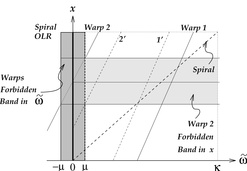
Figure 3: On this figure are presented two pairs of warps which can be coupled with the spiral. At each $x$, we see on the graph that $\tilde{\omega}_{1}+\tilde{\omega}_{2}=\tilde{\omega}_{S}$, and also that $\tilde{\omega}_{1^{\prime}}+\tilde{\omega}_{2^{\prime}}=\tilde{\omega}_{S}$. The grey band at the left arises from the dispersion relation of warps, which cannot propagate where $|\tilde{\omega}|<\mu$.

To this point we have considered the coupling between three waves: the spiral wave, and two low amplitude warp waves which satisfy the selection rules. But any pair of $m=1$ warps obeying the frequency selection rule will also obey the other ones, leaving us potentially with a continuous set of warp pairs coupled to the spiral. The question is now to determine whether one or several couples of warps can be preferentially amplified by the spiral wave, and if so, which one(s) and where. In order to clarify the situation, we present the problem graphically on figure 3. On this figure, each wave is presented by a curve (a segment in the shearing sheet approximation, but this does not lead to a loss of generality). For each curve, $x$ is given by the implicit relation $\tilde{\omega}=\omega-m\Omega(x)$, where we have taken $m_{S}=2$ and $m_{1}=m_{2}=1$. It is an easy matter to check that the slope of the curves describing the warps, at a given $x$, must be twice the slope of the curve describing the spiral. For the reason already explained in section • ‣ 2.2.2, if two warps satisfy the $\tilde{\omega}$-selection rule at some $x$, they satisfy it at any $x$. Since $x$ has its origin at the corotation of the spiral, the curve of the spiral starts from (0,0). The warps cannot propagate in the vertical forbidden band $[-\mu,+\mu]$, since their dispersion relation is (in the infinitely thin disk limit) $\tilde{\omega}_{W}^{2}=\mu^{2}+2\pi G\Sigma q$ (taking into account the finite thickness of the disk and possible compressional effects maintains the existence of such a forbidden band, see e.g. Masset and Tagger 1995). For a given warp, the forbidden frequencies can be converted into a forbidden band in $x$ as shown on figure for warp 2.

We have depicted a narrow forbidden band since $\mu$ is expected to be small compared to $\kappa$ if the rotation curve is nearly flat. In the ideal case where the rotation curve is really flat, $\kappa=\sqrt{2}\Omega$ giving $\mu=0$.

According to the expression of system (I), we see that the coupling can be strong where one or several group velocities vanish. Physically, this corresponds to the fact that the waves take a long time to propagate away from the region where coupling occurs, leaving them ample time to efficiently exchange energy and momentum.

As already mentioned, we shall now use the group velocity of a stellar spiral for the spiral wave, although we keep our purely gaseous coupling coefficient. By doing so, we avoid the tedious handling of a mixed kinetic-hydrodynamic formalism without a great loss of precision. The group velocity of the spiral vanishes near the Lindblad resonances (here at the Outer Lindblad Resonance, OLR) and the group velocity of the warp vanishes at the edge of the forbidden band, where an incident warp must be reflected .

For these reasons we have four qualitatively distinct cases to consider:

Far from the OLR of the spiral:

• We consider two warps, none of which close to its forbidden band;

• Or a pair of warps, one of which lies at the edge of its forbidden band.

At the OLR of the spiral:

• We consider two warps, none of which close to its forbidden band;

• Or a pair of warps, one of which lies at the edge of its forbidden band.

4.2.1 Far from the OLR

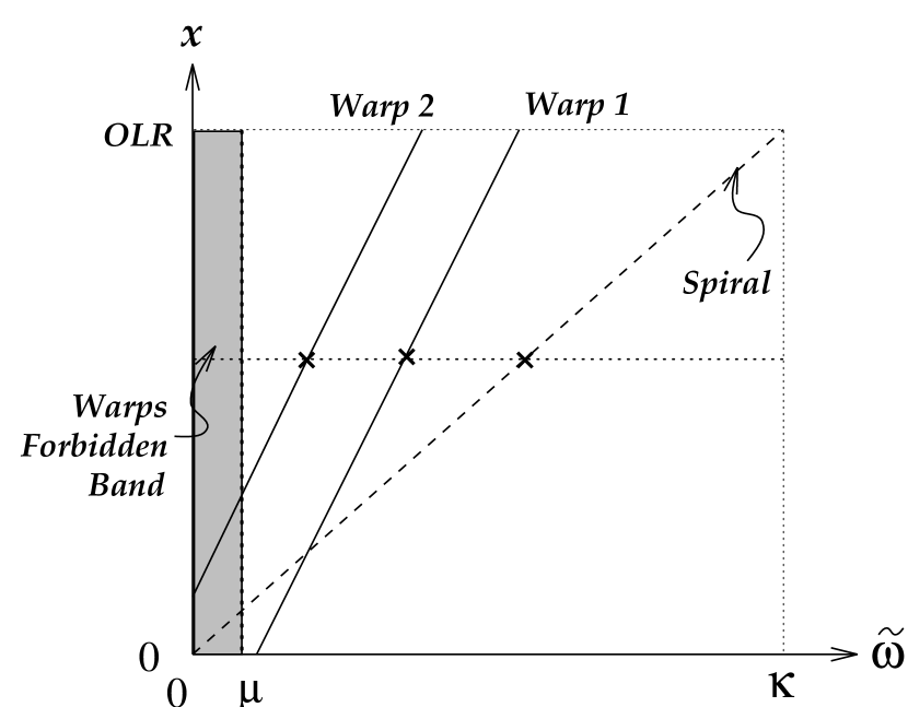
Figure 4: This figure presents the first case studied in the text. We analyze the efficiency of coupling at the radial position given by the horizontal dotted line, far from the OLR of the spiral (top of the diagram). Both warps are far from their forbidden band.

Let us analyze the first case. The graph is presented in figure 4. We choose a value of $x$ such that neither warp is close to its forbidden region. We define $H_{t}$ by $H_{t}^{1/2}=H_{1}^{1/2}+H_{2}^{1/2}$. Summing the two first lines of system (I), and after some transformations, we obtain:

$$\partial_{x}H_{t}^{1/2}=\frac{\tilde{\omega}_{S}\nu_{Z}^{2}}{2K_{1}K_{2}}\frac{1}{\sqrt{c_{g_{1}}c_{g_{2}}}}\frac{\sigma}{\Sigma}H_{t}^{1/2}$$ (4)

Our purpose is to determine whether the coupling will be sufficient in these conditions to extract the warps from the noise level. As long as the warps remain at this low amplitude, their influence on the flux of the spiral is negligible. We then assume that $\sigma/\Sigma$ is constant. This naturally leads us to define an $e$-folding length for the warps. If this length happens to be short (in a sense which will be defined below), the warps can be strongly amplified from the noise level. Here, the $e$-folding length is:

$$\lambda_{e}=\frac{2\sqrt{c_{g_{1}}c_{g_{2}}}K_{1}K_{2}}{\tilde{\omega}_{S}\nu_{Z}^{2}}\frac{\Sigma}{\sigma}$$

Taking into account the expression of $K_{i}$ given in appendix D, and noting that the group velocity of warp $i$ can be written as $c_{g_{i}}=a\kappa/Q\tilde{\omega}_{i}$, we can rewrite this as:

$$\lambda_{e}=4\frac{a}{Q\nu_{Z}^{2}}\sqrt{\biggl{(}1+\frac{\mu^{2}}{\tilde{\omega}_{1}^{2}}\biggr{)}\biggl{(}1+\frac{\mu^{2}}{\tilde{\omega}_{2}^{2}}\biggr{)}}\sqrt{\tilde{\omega}_{1}\tilde{\omega}_{2}}\frac{\Sigma}{\sigma}$$

where we have taken the typical value (see the diagram) $\tilde{\omega}_{S}=\kappa/2$.

Now let us follow these two warps in their motion outward. After traveling over a distance $\lambda_{e}$, their quadratic total flux $H_{t}$ has been amplified by a factor $e^{2}$. Will amplification at this rate be sufficient for the warps to extract a significant fraction of the flux of the spiral ? For this to occur, the spiral and the beat-wave of the warps should be able to maintain a well-defined relative phase as they travel radially, lest the coupling term oscillates and gives alternatively a positive and negative energy flux from the spiral to the warps. We meet here a condition which is the WKB equivalent of the selection rule on the radial wavenumbers: since the WKB wavenumbers of the waves do not a priori obey this selection rule, they will decorrelate over a few radial wavelengths, $k_{x}^{-1}\sim a/\Omega$, where $k_{x}$ is the radial wavenumber of any of the waves involved. Thus if $k_{x}\lambda_{e}$ is small the warps can be strongly amplified before they decorrelate from the spiral, whereas if $k_{x}\lambda_{e}$ is of the order of 1 or larger the coupling will not significantly affect them. Here, we have:

$$k_{x}\lambda_{e}=\frac{4}{Q}\underbrace{\frac{\Omega^{2}}{\nu_{z}^{2}}}_{\sim.1}\underbrace{\biggl{(}\frac{\tilde{\omega}_{1}\tilde{\omega}_{2}}{\Omega^{2}}\biggr{)}^{2}}_{\sim 1}\underbrace{\frac{\Sigma}{\sigma}}_{\sim 10}\sim\frac{4}{Q}\sim 1$$

Then the waves are in an adequate phase condition over one $e$-folding length at best, and we conclude that the warps cannot be extracted from the noise level in this first case.

Figure 5: This figure shows the second case studied in the text. We analyze the efficiency of coupling at the radial position given by the horizontal dotted line, far from the OLR of the spiral (top of the diagram). Now one of the warps is located just at the edge of its forbidden band.

The second case, illustrated in figure 5, still corresponds to coupling far from the OLR of the spiral, but with one warp near the forbidden band. It is an easy matter to check from the linear dispersion relation that the group velocity of a warp near its forbidden band is given by:

$$c_{g}(\Delta x)=\sqrt{\frac{A}{\mu}Q\kappa a\Delta x}$$ (5)

where $\Delta x$ is the distance to the forbidden band. This formula has been obtained in the WKB limit, but we do not expect very different results in the general case. This leads us to replace in the expression of $\lambda_{e}$ a term of the type: $H/\sqrt{c_{g_{2}}}$ by an integral of the type:

$$\int_{0}^{H}\frac{d(\Delta x)}{c_{g_{2}}^{1/2}(\Delta x)}$$

We have adopted the length scale $H$ because it corresponds to the range over which equation (5) is valid, close to the forbidden band.

The ratio of these two quantities is:

$$\frac{4}{3}\biggl{(}\frac{\Omega\kappa}{A\mu}\biggr{)}^{1/4}\frac{1}{Q^{3/4}}$$

and is typically of the order of $1$ (the exponent $1/4$ does not allow it to change very much). Furthermore, the coefficient $\sqrt{\tilde{\omega}_{1}\tilde{\omega}_{2}/\Omega^{2}}$ is now about $\sqrt{\mu/\Omega}$, i.e. about $1/2$. This is not sufficient to make the value of $q\lambda_{e}$ much smaller than $1$.

Thus we can conclude that far from its OLR the spiral cannot transfer its energy and angular momentum to the warps.

4.2.2 Near the OLR

We turn now the last two cases, corresponding to coupling close to the Outer Lindblad Resonance of the spiral. What does close mean here ? We said that we must study separately the behavior of coupling near the OLR because the group velocity of the spiral in a stellar disk tends to zero as its approaches the resonance. In fact it does not really vanish (Mark, 1974), but we can in a first approximation consider that it does, with a decay length scale of the order of the disk thickness. Since this behavior is associated with the resonant absorption of the spiral wave at its OLR, by beating with the epicyclic motion of the stars, we expect that it should survive even in a realistic mixture of stars and gas. From the dispersion relation for a stellar spiral given by Toomre (1969), and using the asymptotic expression of Bessel functions, one can write the group velocity of the spiral near its OLR as:

$$c_{g_{S}}\simeq a\sqrt{Q}\biggl{(}\frac{4|A|}{\kappa}\biggr{)}^{3/2}\biggl{(}\frac{r_{OLR}-r}{r}\biggr{)}^{3/2}$$

So that now the group velocity is a power $3/2$ of the distance to OLR.

We can slightly transform our expression of $\lambda_{e}$, the $e$-folding length of the preceding section, as:

$$\lambda_{e}=\frac{4a}{Q\nu_{z}^{2}}\sqrt{\tilde{\omega}_{1}\tilde{\omega}_{2}}\frac{\Sigma^{1/2}K_{S}}{H_{S}^{1/2}}c_{g_{S}}^{1/2}$$

This expression is more appropriate in this new situation, since (at least when the fluxes of the warps remain small compared to the flux of the spiral) $H_{S}^{1/2}$ is constant (while $\Sigma/\sigma$ is not) and now $c_{g_{S}}$ varies. As before, we have to see how many $e$-folding lengths are contained in a scale length of the order of $a/\Omega$, where we can use the above expression for the spiral group velocity. Then we have to replace $H/c_{g_{S}}^{1/2}$ in our previous estimate by $\int_{0}^{H}dx/c_{g_{S}}^{1/2}(x)$, leading us to multiply the number of $e$-folding lengths over a scale $H$ by:

$$\int_{0}^{1}\frac{dx}{x^{3/4}}=4$$

Furthermore, we had taken in the previous section the mean value $\tilde{\omega}_{S}=\kappa/2$. Now since we are close to the OLR we have to take $\tilde{\omega}_{S}=\kappa$. Finally, with our typical figures, instead of having only one $e$-folding length for $H_{t}^{1/2}$ over a scale length $H$, we find eight such $e$-folding lengths, i.e. near the OLR the flux of the warps can be multiplied by $e^{2\times 8}=10^{7}$. Of course this flux cannot become arbitrarily large, so that when it reaches the spiral flux we can consider that most of the spiral flux has been transferred to the warps. Even though our factor of $10^{7}$ could be reduced by many effects, we consider that mode coupling near the OLR is efficient enough to allow the warps to grow from the noise level until they have absorbed a sizable fraction of the flux of energy and angular momentum carried by the spiral from the inner regions of the galactic disk.

We now have to check in more details the effect of the localization of the coupling coefficient. Indeed from the system (I) we see that, if the amplitudes of the waves varied more rapidly than the coupling coefficient, their oscillations would reduce or even cancel over a given radial interval the efficiency of the coupling. This must be considered because the same effect which gives a vanishing group velocity for the spiral near its OLR also causes their radial wavenumber to diverge.

However, from the expression above for the group velocity of the spiral, we see that:

$$\frac{\partial k_{r}}{\partial r}\sim\frac{\partial k_{r}}{\partial\omega}\sim(r_{OLR}-r)^{-3/2}$$

so that

$$k_{r}\sim(r_{OLR}-r)^{-1/2}\quad.$$

Now the phase of the spiral, in the WKB approximation, varies as

$$\exp{(\imath\int k_{r}dr)}$$

and the integral converges, so that in fact the phase tends to a finite limit (instead of varying rapidly as one might think from the divergence of $k_{x}$). Thus in the expressions on the RHS of system (I), the quantity which gives the dominant behaviour is indeed the (integrable) divergence of the coupling coefficient, in the vicinity of the OLR. This justifies that, in our estimates, we have integrated over the variations of this coefficient, keeping the other quantities approximately constant. It also justifies our statement, in section 2.2, that the generation of the warps is impulsive-like.

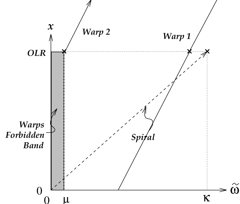
Figure 6: This figure shows the final result of our study. The coupling is strongly efficient at the OLR, and only there, and results in a conversion of the spiral into two warp waves, at $\tilde{\omega}_{2}=\mu$ and $\tilde{\omega}_{1}=\kappa-\mu$.

This does not tell us yet which couple of warps is preferentially amplified at OLR, according to their frequencies. In fact the coupling coefficient still depends on these frequencies, through the term in $\sqrt{\tilde{\omega}_{1}\tilde{\omega}_{2}}$. This factor, associated with the group velocities of the warps, further increases the efficiency for the most “external” pair: $[\omega_{1}=\kappa-\mu,\omega_{2}=\mu]$ (by a factor $\sim 2$ compared to the most central pair of warps if we assume $\mu/\Omega\sim 1/4$). This difference is amplified geometrically at each $e$-folding length, and thus finally we can consider that the pair $[\mu,\kappa-\mu]$ is preferentially emitted at the OLR. This result is illustrated in figure 6.

Now we have determined how and where the spiral is “converted” into warps. But we still have to find how the energy is distributed between the warps, and in which direction they propagate. On figure 6 we have illustrated the warp 2 with an outward-pointing arrow, since we know that it is necessarily emitted outward due to the presence of its forbidden band. But warp 1 can consist of two waves, propagating inward as well as outward, and we must now consider the detailed balance of the energy transferred to the three warps. This can be done using the conservation of angular momentum. The relation between the energy flux $H$ and angular momentum flux $J$ is, for the warps as well as the spiral (Collett and Lynden-Bell 1987):

$$J=\frac{mH}{\omega}$$

since angular momentum and energy are advected at the same velocity $c_{g}$. Angular momentum conservation gives:

$$J_{S}=J_{1}^{(+)}+J_{1}^{(-)}+J_{2}$$

where $J_{S}$ is the momentum flux lost by the spiral, while $J_{1},\ J_{2}$ are the fluxes gained by the warps, and the $(+)$ et $(-)$ upper-scripts denote respectively the warps 1 emitted outward and inward. Writing $J_{1}=J_{1}^{(+)}+J_{1}^{(-)}$, and using the the fact that the waves 1 have the same frequency, we get $J_{1}=m_{1}H_{1}/\omega=H_{1}/\omega_{1}$, giving from energy and momentum conservation the system of equations:

$$\left\{\begin{array}[]{l}\displaystyle H_{1}+H_{2}=H_{S}\\ \displaystyle H_{1}/\omega_{1}+H_{2}/\omega_{2}=2H_{S}/\omega_{S}\end{array}\right.$$

Defining $\beta_{1}$ and $\beta_{2}$ as the ratios $H_{1}/H_{S}$ and $H_{2}/H_{S}$, we find $\beta_{i}=\omega_{i}/\omega_{S}$.

Using the frequencies of the preferred pair of warps leads to:

$$\left\{\begin{array}[]{l}\displaystyle\beta_{1}=\frac{\Omega+\kappa-\mu}{2\Omega+\kappa}\\ \displaystyle\beta_{2}=\frac{\Omega+\mu}{2\Omega+\kappa}\end{array}\right.$$

A strictly flat rotation curve would give: $\beta_{1}=0.71$ and $\beta_{2}=0.29$, while a nearly flat rotation curve with $\mu/\Omega=0.25$, would give: $\beta_{1}=0.63$ and $\beta_{2}=0.37$.

Now it is an easy matter to check that the fluxes carried away by warps $1^{(+)}$ and $1^{(-)}$ are equal. The easiest way to do it is to write for the pair of warps $1$ a system similar to the one used above. This system is degenerate, but introducing a slight offset between the frequencies and making it tend to zero we find that they share equally the flux $\beta_{1}H_{S}$. Physically, this corresponds to the fact that the source of the waves is “impulsional” (very localized), so that they are emitted equally without a preferred direction in space.

From the numerical values given above, we can deduce that each of the three waves (two emitted, one reflected) carries away one third of the flux extracted from the spiral, as a very good approximation.

4.3 Detailed physics at the OLR

The situation exposed above is idealized. Two remarks modify the simple computations, but should not qualitatively alter the main physical conclusions.

• First, the group velocity of the spiral does not really vanish at the OLR. This has been investigated by Mark (1974), who showed that the group velocity of the spiral at the OLR was about a few kilometers per second (typically 10 times lower than the value it has far from the OLR). This leads us to replace the factor $4$ in our computation by about $\sim\sqrt{10}$. Nevertheless, we still have a “large” number of $e$-folding lengths in the region “just before” the OLR.

• The spiral, as it approaches its OLR, is linearly damped through Landau effect. Mark (1974) gives an absorption length by Landau damping which has typically the same order of magnitude as the $e$-folding length we find for non-linear coupling. The two processes can thus compete, the spiral losing part of it energy and momentum flux to the stars (heating them and forming an outer ring), and to non-linearly generated warps, at comparable rates. It is thus very likely that the dominant process (non-linear coupling or Landau damping) will depend on the local characteristics of the galaxy under consideration.

5 Comparison with observations

In this section we derive the expected characteristics of the warps produced by the coupling process. Let us first summarize the main results obtained in the previous section. The reader can also refer to figure 7 where the situation is depicted.

Figure 7: This figure shows the spiral wave and the three warp waves excited near its OLR by non-linear coupling. See the text for more details.

• The spiral wave travels outward until it reaches its OLR. Before it reaches it, the coupling with warps is too weak to affect the spiral.

• When it reaches the OLR (more precisely within a distance of the order of $a/\Omega$ from the OLR) the spiral slows down and is efficiently coupled with warps. This results in the “conversion” of the spiral into three warps which carry the incident flux of the spiral away from the coupling region: two warps at frequency $\kappa-\mu$, traveling respectively outward and inward, and the last warp at frequency $\mu$, which is emitted outward.

• The flux absorbed from the spiral is approximately equally shared by the three warps, for reasons of conservation of angular momentum and energy.

• In the following we will neglect the absorption of the spiral wave by Landau damping. Thus our results on the warps amplitudes will be optimistic, but still give results of the correct order of magnitude since the length scale of Landau damping and non-linear coupling are similar.

5.1 Amplitude of the warp

We will now derive a rough prediction of the warp displacement resulting from our mechanism. For each of the three warps we can write:

$$c_{g_{W}}E_{W}\simeq\frac{1}{3}c_{g_{S}}E_{S}$$

where the factor $1/3$ comes from the result (see section 4.2.2) that the three warp waves share nearly equally the flux extracted from the spiral (the rest of the flux of the spiral being absorbed by Landau damping, as discussed in section 4.3).

In order of magnitude, the flux of the spiral is given by:

$$H_{S}=c_{g_{S}}E_{S}\sim a\times a^{2}\Sigma_{disk}\biggl{(}\frac{\sigma}{\Sigma_{disk}}\biggr{)}^{2}$$

Similarly, the fluxes of the warps emitted outward are:

$$H_{W}=c_{g_{W}}E_{W}\sim a\times\tilde{\omega}_{W}^{2}\Sigma_{out}Z^{2}$$

In these expressions, $\Sigma_{disk}$ is the unperturbed surface density of the stellar disk, where the spiral propagates, and $\Sigma_{out}$ is the unperturbed surface density of the external HI disk, where the two emitted warps propagate.

Now if we adopt a radial dependence of $\Sigma_{out}$ such as given by Shostak and Van der Kruit (1984), that we will very roughly describe by :

$$\Sigma_{out}(r)=\Sigma_{0}\exp[-(r-r_{0})/d]$$

where $r_{0}$ is the radius of the optical limit of the disk, $d$ the decaying length of surface density (a sizable fraction of $r_{0}$), we can deduce an approximate radial dependence of the deviation $Z$. We find :

$$\biggl{(}{Z\over H}\biggr{)}^{2}=\biggl{(}\frac{\sigma}{\Sigma_{disk}}\biggr{)}^{2}\frac{\Sigma_{disk}}{3\Sigma_{0}}e^{(r-r_{0})/d}$$

$$\Sigma_{disk}\sim 75\;\;M_{\odot}.\rm{pc}^{-2}$$

and

$$\Sigma_{0}\sim 10^{-20}\mbox{part}.cm^{-2}$$

(see e.g. Huchtmeier and Richter 1984 or Shostak and Van der Kruit 1984).

and we take as a value for the amplitude of the spiral $\sigma/\Sigma_{disk}\sim 0.1$ (but it could be larger than this widely adopted value, see Strom et al. 1976). This leads us to:

$$Z/H\sim{1\over 2}e^{[(r-r_{0})/2d]}$$

Of course $\Sigma_{out}$ decreases progressively as the warps propagate outward, and $Z$ accordingly grows to preserve the flux.

The dependency found above is typical of what is observed in isolated spiral galaxies. It is noteworthy — and we believe that this has not yet been noticed — that the flux of the spiral waves is of the same order of magnitude as the flux of the warps. We consider this coincidence as a strong point in favor of our mechanism — independently of its details —, and a challenge to any alternate model.

5.2 Expected characteristics of the corrugation

The computations concerning the reflected warp are slightly different. One should remember that it propagates in a region where both stars and gas are present, a fact which cannot be neglected when discussing its characteristics. In a previous paper (Masset and Tagger, 1995) we discussed the propagation of warps in a two-fluid disk. We found two types of waves: the first type corresponds to waves where both fluids move essentially together, while the second type corresponds to waves where the fluids move relative to each other; assuming that the stellar disk is much warmer and much more massive than the gaseous one, in this type of wave the stars stay essentially motionless while the gas moves in their potential well. We consider that this wave, which we call the corrugation mode, will be excited much more easily than the previous ones, since it moves much less mass and thus its amplitude for a given energy must be much higher. Its dispersion relation is:

$$\tilde{\omega}^{2}=\mu^{2}+4\pi G\rho_{*}+2\pi G\Sigma_{g}q+\frac{\tilde{\omega}}{\tilde{\omega}^{2}-\kappa^{2}}{a_{g}^{2}q^{2}}$$

where the subscripts $g$ and $*$ apply to gaseous and stellar values, and where $\rho_{*}$ is the stellar density at midplane. Because of the moderate thickness of the stellar disk, the square frequency $\nu_{z}^{2}=4\pi G\rho_{*}$ is much larger than the other characteristic frequencies of the problem, and in particular larger than the frequency $\tilde{\omega}\simeq\kappa-\mu$ of the wave which can be non-linearly excited. A solution can nevertheless be found because inside the OLR of the warp the last term in the dispersion relation is negative, and can for large enough values of $q$ balance the dominant term $\nu_{z}^{2}$. Neglecting the self-gravity of the gas, and writing $\tilde{\omega}^{2}\ll 4\pi G\rho_{*}$ (a realistic assumption since the ratio of these quantities is about one tenth), we find:

$$q=\frac{\sqrt{4\pi G\rho_{*}}}{a_{g}}\frac{\sqrt{\kappa^{2}-\tilde{\omega}^{2}}}{\tilde{\omega}}$$

Assuming a $sech^{2}(z/H)$ vertical stellar density profile (i.e. the disk is dominated by the local stellar gravity, which is a reasonable assumption), this can be rewritten as:

$$\frac{\lambda}{H_{*}}=4.4\frac{a_{g}}{a_{*}}\frac{1}{\sqrt{\kappa^{2}/\tilde{\omega}^{2}-1}}$$ (6)

Taking $a_{g}/a_{*}\sim.2$, and $H_{*}$ of the order of one kiloparsec, we find an order of magnitude of one kiloparsec for the wavelength of the corrugation. This is consistent with the observed wavelength for the corrugation, in the Milky Way (Quiroga and Schlosser 1977, Spicker and Feitzinger 1986) or in other galaxies (Florido et al.  1991a). Despite the observations by Spicker and Feitzinger of a one kiloparsec corrugation in our galaxy, it seems that the typical wavelength of corrugation is rather about 2 kiloparsecs, or even larger (Florido et al.  1991b). The discrepancy of $\leavevmode\nobreak\ 2$ between observations and our estimate could be due either to the magnetic field which affects the gas motions and thus should imply the use of magnetosonic speeds instead of the acoustic speed, or to a lack of resolution of some observations. From equation (6), we find that the wavelength of corrugations increases as we approach the edge of the optical disk, in good agreement with observations.

Now let us give an order of magnitude of the expected amplitude of the corrugation. As already explained, we can write that its flux is about one third of the spiral flux. Now the flux of the corrugation is roughly given by (the index $c$ is for corrugation):

$$H_{c}=c_{g_{c}}E_{c}$$

where:

$$c_{g_{c}}=\biggl{|}\frac{\partial\tilde{\omega}}{\partial q}\biggr{|}\simeq\frac{\tilde{\omega}}{q}\simeq\frac{\kappa}{q}=\frac{\kappa H_{*}}{qH_{*}}\sim a_{*}$$

since $qH_{*}\sim 1$, and:

$$E_{c}=\frac{1}{2}\nu_{z}^{2}\Sigma_{g}Z^{2}$$

Hence:

$$Z^{2}\sim\frac{\Sigma_{*}}{\Sigma_{g}}\frac{a_{*}^{2}}{\kappa^{2}}\biggl{(}\frac{\sigma}{\Sigma_{*}}\biggr{)}^{2}$$

which gives, taking into account $H_{*}/R\sim\kappa^{2}/\nu_{z}^{2}$:

$$Z=\sqrt{\frac{\Sigma_{*}}{\Sigma_{g}}\frac{H_{*}}{R}}H_{*}\biggl{(}\frac{\sigma}{\Sigma_{*}}\biggr{)}$$

Taking $H_{*}\sim 1\mbox{ kpc}$ and $\sigma/\Sigma_{*}\sim.1\mbox{ to }.2$, we obtain an expected amplitude for the corrugation of about one hundred parsecs, which is typically the observed value. Note that, as discussed above, energy can also be given to the other modes, involving both the gas and the stars, for the reflected warp. Their expected wavelength is larger than the disk radius, so that their line of nodes should be almost straight, corresponding to the observations of Briggs (1990), and so that the corrugation can easily be detected when superimposed on such large scale bending waves.

5.3 Straight line of nodes

We have found thus far that our mechanism leads to results that fit well the observations for the amplitudes of the “outer” warps (the two waves emitted beyond the OLR of the spiral) and of the corrugation, and for the wavelength of the corrugation. We now turn to the wavelength of the outer warps. Actually the line of nodes of the observed warps is always nearly straight, leading to radial wavelengths larger than the galactic radius. This is known as the problem of the straight line of nodes, and is one of the most serious challenges to models of warps. In his work on the “Rules of Behavior of Galactic Warps”, Briggs (1990) has emphasized this remark: the line of nodes of the outside warps appears nearly straight or with a slight spirality, always almost leading. Later observations have shown that outside warps could also be slightly trailing, but always nearly straight. This can be interpreted from our mechanism, which predicts the emission of two warps outward from the OLR. In fact, the frequency of the first warp is $\mu$, leading from the dispersion relation to a wavevector $k_{x}=0$, hence a straight line of node. The second one is emitted at $\tilde{\omega}\simeq\kappa-\mu$, i.e. near its OLR. From the dispersion relation of warps taking into account the compressibility effects near the OLR (see e.g. Masset and Tagger 1995), we see that $k_{x}$ must tend to zero in order to balance the behavior of the resonant denominator, thus also leading to a straight line of nodes.

Of course this is a qualitative and simple interpretation, since we use results obtained in the framework of the WKB assumption (tightly wound waves) where $k_{x}$ is precisely not allowed to become small. Hence this discussion about the straight line of nodes is just the very beginning of a more complete work which should take into account non-WKB effects and the cylindrical geometry. This work is in progress, using the numerical code introduced in Masset and Tagger 1995. Finally, we should mention that the combination of two warps outside OLR can easily justify the large and arbitrary jump in the line of nodes across the Holmberg radius observed by Briggs, since the relative phase between warps 1 and 2 is arbitrary.

6 Discussion

6.1 Summary of the main results

We have written the non-linear coupling coefficients between a spiral and two warps, taking into account the finite thickness of the galactic disk and the three dimensional motion in a warp. The efficiency of this mechanism is too weak in the stellar disk, except at its outer edge where the spiral slows down near its OLR and can be efficiently coupled to warps and extract them from the noise level, transferring to them a sizable fraction of its energy and angular momentum (with the rest transferred to the stars by Landau damping). As a net result we can consider that the spiral is transformed into two warps. One of them receives a third of the energy of the spiral and can propagate only outward. The other receives the remaining two thirds of the energy of the spiral, and splits into one wave traveling outward and one traveling inward, which we tentatively identify as the corrugation observed in many galaxies.

Order of magnitude estimates of the respective amplitudes of the outer warp (in the HI layer) and of the inner one (the corrugation), as well as of their wavelengths, lead to values in good agreement with observations. In particular we find from the observed amplitudes that the energy and angular momentum fluxes of the spiral and the warps are comparable, a result which receives a natural explanation in our model.

The expected long wavelength of the outer warp is in agreement with the observed trend to forming a straight line of nodes. Furthermore, our mechanism justifies the phase discontinuity of the warp at crossing the Holmberg radius (since the Holmberg radius is expected to be close to the Outer Lindblad Resonance of the spiral, where our mechanism takes place).

6.2 What about the halo ?

In the preceding sections we have not mentioned the role of a massive halo. We will not discuss a misalignment between the disk and the principal plane of the halo, since such a misalignment was introduced in an ad hoc model by Sparke and Casertano (1984) in order to explain the continuous excitation of the warp in isolated galaxies. Our mechanism does not require such an hypothesis.

A typical halo is about ten times more massive than the disk. If this halo has a spherical symmetry, it does not affect the vertical restoring force and thus leaves our results unchanged. On the other hand a flattened halo would give rise to a strong restoring force for a test particle (or a disk) displaced from the equatorial plane. The vertical oscillation frequency $\mu$ would be about three times the epicyclic frequency. Hence the forbidden band of figures 4–6 would invade more than the whole disk. Our analysis would then have to be altered, but we believe that its main result would remain valid.

Indeed, in order to find two bending waves that would propagate in the vicinity of the OLR of the spiral, we might invoke the “slow” branch of the warp dispersion relation, which uses intensively the compressional behavior of the gas (let us emphasize that we have already made use of this slow branch to find the wavelength of corrugation, which is in the same manner a bending wave of the gas in the deep potential well of the stars). This would not strongly change the expected efficiency of our mechanism, and would even rather increase it slightly, since we would be dealing with slower modes. Another solution would be to consider the pair of warps $[-\mu,\kappa+\mu]$, which are both simultaneously propagating (with the former being retrograde). The efficiency of coupling with such a pair would be, in our framework (shearing sheet and steady state) exactly the same as the one we derived for the pair $[\mu,\kappa-\mu]$. Now the details of the scenario would change a little. We would have only one wave emitted outward and two inwards, but the order of magnitude of their amplitudes would not change. Note that observations of corrugation in external galaxies (Florido et al. 1991a) seem to reveal two distinct wavelength for corrugation waves.

Another matter concerns the response of the halo to the warp. A fully consistent treatment of this problem should be numerical. However, it is possible to get analytical trends by considering the halo as a thicker (and then warmer) disk than the stellar/gaseous disk. This can be done using the two-fluid dispersion relation of warps (see Masset and Tagger 1995). The two-fluid dispersion relation reveals three modes:

• A mode which involves essentially the thinner and lighter component, leaving the other one (the halo) nearly motionless. This mode is the one described in the preceding lines, and corresponds to the gaseous corrugation within the stellar disk as well as to the compressional mode of the whole disk (stars plus gas) in the rest potential of the halo.

• The classical two modes (slow and fast) of the one-fluid analysis, which involve similar motions of both fluids. This means that the halo would participate in the different warps, as well as in the spiral, and formally the problem would be the same as the one described throughout this paper, with the difference that we would have to use the total surface density, involving the projected one of the halo, and the total thickness, which is the halo thickness, of the order of $r/2$. Each of these quantities should then be multiplied by about ten. Hence the test particle frequency $\nu_{Z}$ would remain the same, since it is proportional to $\sqrt{\Sigma/H}$. We then see on equation (4) that each factor would remain unchanged, except the group velocities whose expression would probably be slightly different, but could not differ much from the sound speed; hence the e-folding length would have the same behavior and order of magnitude. Furthermore, a participating halo would give a more efficient and simple explanation to the problem of the straight line of nodes, since the wavelength of warps, for a given excitation frequency, increases with the surface density.

Figure 8: In this figure we present the three modes for bending waves in a two-fluids system (disk –denoted by a star– and halo –denoted by a h–). We have adopted the following parameters: $\Sigma_{h}/\Sigma_{*}=10$, $\mu^{2}/\kappa^{2}=0.1$, $\tilde{\omega}/\kappa=0.75$. The results (the elongation $Z_{h}$ of the halo over the elongation $Z_{*}$ of the disk, and the wavelength) are presented as a function of the ratio $a_{*}/a_{h}$. For a typical galaxy, this ratio should be about $0.2$. The solid line represents the classical infinitely thin one-fluid mode. We see that its wavelength is far greater than the disk radius (hence it could be a beginning of the justification of the straight line of nodes problem) and that the disk and halo have nearly the same elongation. The dotted line represents the one-fluid compressional mode. Its wavelength is about four times the disk radius, and we see that the halo is more warped than the disk since the halo elongation is about $1.6$ that of the disk. Finally the dashed curve represents the corrugation-like wave, i.e. here the “corrugation” of the whole disk (stars and gas) in the rest potential of the halo, which appears to be in that case nearly motionless ( $Z_{h}\ll Z_{*}$).

Figure 8 shows that the participation of the halo to the global modes (i.e. the two waves corresponding to the one-fluid ones) is as strong as or stronger than that of the disk. Furthermore the wavelengths of these modes agree with the observations of a straight line of nodes. However, this figure has been obtained in the WKB assumption and moderately thick disk formalism (Masset and Tagger 1995), which are both far too rough in this case, so that a numerical solution taking into account the halo response would be necessary.

In the same manner, if we want to estimate the coupling efficiency taking into account the halo, a problem is a determination of $\sigma/\Sigma$ for the spiral involving a participating halo. If we assume a behavior of matter independent of $z$, then $\sigma/\Sigma$ should still be about $0.2$, but once again only a numerical solution would allow us to give the real vertical profile of perturbed quantities in the spiral and in the warps. Furthermore, the problem is much more complex if we want to treat it fully correctly, since for distances to the galactic center less than the Holmberg radius we have to cope with three fluids: the halo, the stars and the gas, so the method which consists in treating the disk as a unique fluid will give only approximate results.

Nevertheless, despite the large number of allowed modes of propagation of bending waves in this realistic case, we see that global modes (i.e. involving a motion of the halo) will lead to the same efficiency as found in this paper. Numerical simulations would be needed to give an accurate evaluation of the e-folding length and to determine the fraction of incident energy that each wave carries away.

Finally, let us mention that the halo should be a collisionless fluid (i.e. star-like and not gas-like) if we still want the spiral to slow down at the OLR. Observations suggesting that the halo or outer bulge is composed of very low mass stars would confirm this hypothesis (see e.g. Lequeux et al. 1995).

6.3 Suggested observations for checking the spiral-warps coupling mechanism

In this paper we have shown that the spiral wave is converted into bending waves observed as an outer HI warp and a corrugation wave. We have already emphasized the observational fact that the fluxes of these three waves have the same order of magnitude for a typical galaxy. It would be interesting to test this coincidence with a better accuracy, and to search for a correlation between the fluxes of the spiral, the warp and the corrugation. The fluxes can be straightforwardly obtained from such observables as the disk surface density, the rotation curve (which gives values for $\kappa$ and $\mu$), the disk thickness, the perturbed surface density of the spiral (see e.g. Strom et al.  1976), and the deviation of the disk to the equatorial plane — although some of these quantities are better measured in face-on galaxies, and others in edge-on ones, making a complete set of observations in an individual galaxy a challenge. A correlation between the fluxes for a significant number of galaxies would be a strong argument for our mechanism.

Appendix A Formal derivation of the coupling coefficient

A.1 Derivation without the shear terms

We use the hydrodynamical equations (continuity and Euler) and the Poisson equation.We write the first two equations in tensor formalism, in order to avoid too lengthy expressions. The continuity equation is:

$$\partial_{t}\rho+\partial^{i}(\rho V_{i})=0$$ (7)

where the vector $V_{i}$ ($i=1,2,3$) is a tensor which represents $(U,V,W)$, and where we implicitly sum over repeated indices (Einstein’s convention).

The Euler equation is:

$$\frac{\partial V^{i}}{\partial t}+V^{j}\partial_{j}V^{i}+2\epsilon^{ijk}\Omega_{j}V_{k}=-a^{2}\frac{\partial i[\rho_{0}(1+s)]}{\rho_{0}(1+s)}-\partial^{i}\phi$$ (8)

In this expression the last term of the L.H.S. represents the Coriolis acceleration, and $\epsilon^{ijk}$ the Levi-Civita symbol. We also introduce a convenient notation, $s=\rho/\rho_{0}$. The reader can note that, in the convective derivative $(V.\nabla)V$, we have not written the shear terms. We neglect them in this first approach, and we will check their influence at the end of this section.

In the Euler equation the pressure term can be expanded to second order as:

$$-a^{2}\biggl{[}(1-s)\partial^{i}s+\frac{\partial^{i}\rho_{0}}{\rho_{0}}\biggr{]}$$

Finally, the Poisson equation is:

$$\Delta\phi=4\pi G\rho$$ (9)

We want to know the energy injection rate into warp 1 from the spiral and the warp 2. In the linear regime, we would have: $\partial_{t}E_{1}=0$. Here, we will have a non-vanishing expression due to the presence of the spiral and warp 2.

Since we treat the warp 1, we expand the hydrodynamic equations to second order in the perturbed quantities and project them onto $e^{-i\omega_{1}t}$.

For the continuity equation (7) this gives:

$$\frac{\partial\rho_{1}}{\partial t}+\partial_{i}(\rho_{0}V_{1}^{i})+\partial_{i}(\rho_{S}V_{2}^{i*})+\partial_{i}(\rho_{2}^{*}V_{S}^{i})=0$$ (10)

and for the Euler equation (8):

$$\frac{\partial V_{1}^{i}}{\partial t}+V^{j}_{S}\partial_{j}V_{2}^{i*}+V_{2}^{j*}\partial_{j}V_{S}^{i}+2\epsilon^{ijk}\Omega_{j}V_{k_{1}}=$$ (11)

$$-a^{2}\partial^{i}s_{1}-\partial^{i}\phi_{1}+a^{2}s_{S}\partial^{i}s_{2}^{*}+a^{2}s_{2}^{*}\partial^{i}s_{S}$$

Our purpose is to write the temporal derivative of an expression which can be interpreted as the energy density of the warp (energy density per unit surface). For this we multiply equation (11) by $a^{2}\rho_{1}^{*}/\rho_{0}$ and equation (10) by $\rho_{0}$, we integrate over $z$, add them and their complex conjugates. This gives:

$$\partial_{t}\int[\rho_{0}(V_{1}^{i}V_{1_{i}}^{*}+a^{2}s_{1}s_{1}^{*})]+\biggl{[}\int\rho_{0}V_{i_{1}}\partial^{i}\phi_{1}^{*}+c.c.\biggr{]}$$ (12)

$$=-\int a^{2}\rho_{0}V_{i_{1}}^{*}\partial^{i}s_{1}-\int a^{2}s_{1}\partial_{i}(\rho_{0}V_{1}^{i*})-\int\rho_{0}V_{1_{i}}^{*}V^{j}_{S}\partial_{j}V^{i*}_{2}$$

$$-\int\rho_{0}V^{*}_{1_{i}}V^{j*}_{2}\partial_{j}V^{i}_{S}+\int\rho_{0}a^{2}V^{*}_{1_{i}}s_{S}\partial^{i}s^{*}_{2}+\int\rho_{0}a^{2}V^{*}_{1_{i}}s_{2}^{*}\partial^{i}s_{S}$$

$$-\int a^{2}s_{1}^{*}\partial_{i}(\rho_{S}V^{i*}_{2})-\int a^{2}s^{*}_{1}\partial_{i}(\rho_{2}^{*}V^{i}_{S})+c.c.$$

In this tensorial notation we will freely use the rule of integration by part (i.e. transpose derivative operators with a change of sign) in the linear terms of this equation: indeed if the index $i$ is $z$, this is really an integration by parts; on the other hand if $i=x$ or $y$ the derivative is just a multiplication by $ik_{i}$ (in our WKB analysis), so that e.g. :

$$s_{1}\partial_{i}(\rho_{0}V_{1}^{i*})=-\rho_{0}V_{1}^{i*}\partial_{i}s_{1}\quad.$$

Furthermore, we must remember that the integration is only over $z$, so that we do not need to worry about boundary terms the integration by parts would introduce in an integration over $x$, and which would represent energy and momentum flux at the radial boundaries of the integration range.

However, we cannot blindly apply this simple formal integration by parts on the non-linear terms. A careful look at the details of the integration by parts for each value of the index $i$ is necessary. For the dimensions ($i\equiv y$ and $i\equiv z$) the formal integration by parts would give correct results, even on the non-linear terms. But for $i\equiv x$, an integration by part would imply a selection rule of the type $k_{x_{S}}=k_{x_{1}}+k_{x_{2}}$, and we have intentionally avoided such an hypothesis. Since we want to stay, for simplicity, in the framework of tensorial formalism, we have to perform transformations that are correct whatever the index $i$ and we do not integrate by parts the non-linear terms in this first part of the derivation.

Equation (A6) already has the form we want : the first term in its L.H.S. is the temporal derivative of the kinetic and internal energy of warp 1. We can note that the term linked to Coriolis acceleration has vanished, since the Coriolis force is always normal to the velocity and thus does not work.

The second term in the L.H.S. must be rewritten to be interpreted as the temporal derivative of the potential energy. We integrate it by parts and then use equation (10) to transform the result. We can also note that the first two terms of the R.H.S vanish together (integrating one of them by parts). We obtain:

$$\partial_{t}\int[\rho_{0}(V_{1}^{i}V_{1_{i}}^{*}+a^{2}s_{1}s_{1}^{*})]+\biggl{[}\int\phi_{1}\partial_{t}\rho_{1}^{*}+c.c.\biggr{]}$$ (13)

$$=-\int\rho_{0}V_{1_{i}}^{*}V^{j}_{S}\partial_{j}V^{i*}_{2}-\int\rho_{0}V^{*}_{1_{i}}V^{j*}_{2}\partial_{j}V^{i}_{S}+\int\rho_{0}a^{2}V^{*}_{1_{i}}s_{S}\partial^{i}s^{*}_{2}$$

$$+\int\rho_{0}a^{2}V^{*}_{1_{i}}s_{2}^{*}\partial^{i}s_{S}-\int a^{2}s_{1}^{*}\partial_{i}(\rho_{S}V^{i*}_{2})-\int a^{2}s^{*}_{1}\partial_{i}(\rho_{2}^{*}V^{i}_{S})$$

$$+\int\phi_{1}^{*}\partial_{i}(\rho_{S}V_{2}^{i*})+\int\phi_{1}^{*}\partial_{i}(\rho_{2}^{*}V_{S}^{i})+c.c.$$

The second term in the L.H.S still does not appear as the time derivative of a potential energy. We have to use the Poisson equation, which we have not used yet.

If we write $S(x^{i}-x^{i}_{0})$ for the potential created at point $x^{i}$ by a unit mass located at point $x^{i}_{0}$, then:

$$\phi=S*\rho$$

where $*$ represents the convolution operator.

Thus, $\phi_{1}=S*\rho_{1}$, $\phi_{S}=S*\rho_{S}$, etc….

We write $\cal L(\rho,\rho^{\prime})$ the form:

$${\cal L}(\rho,\rho^{\prime})=\int_{E}\rho^{*}(\@vec{r})[S*\rho^{\prime}](\@vec{r})d^{3}\@vec{r}$$

where the index $E$ indicates that the integral extends over the whole space. Using the fact that $S$ is a real function with spherical symmetry, it is an easy matter to check that (by writing explicitly the convolution and exchanging the integrals):

$${\cal L}(\rho,\rho^{\prime})={\cal L}(\rho^{\prime},\rho)^{*}$$

Hence $\cal L$ is a variational form, and one can write the following equalities:

$$\int\phi_{1}^{*}\partial_{t}\rho_{1}={\cal L}(\partial_{t}\rho_{1},\rho_{1})={\cal L}^{*}(\rho_{1},\partial_{t}\rho_{1})$$

(whether the integral extends only over $z$ or over the whole space, since the integrated quantity does not depend on $x$ or $y$).

Now:

$$S*\partial_{t}\rho_{W}=\partial_{t}(S*\rho_{W})$$

since $S$ is time independent. This is linked to the use of the Poisson equation, i.e. to the fact that the potential propagates instantaneously. Then one can write:

$$\int\phi_{1}\partial_{t}\rho_{1}^{*}=\int\rho_{1}^{*}\partial_{t}\phi_{1}$$

Thus we see that we can write this term as a potential energy associated to the warp, and this gives:

$$\partial_{t}\int\rho_{0}\biggl{[}(V_{1}^{i}V_{1_{i}}^{*}+a^{2}s_{1}s_{1}^{*})+\biggl{(}\frac{1}{2}s_{1}^{*}\phi_{1}+c.c.\biggr{)}\biggr{]}$$ (14)

$$=-\int\rho_{0}V_{1_{i}}^{*}V^{j}_{S}\partial_{j}V^{i*}_{2}-\int\rho_{0}V^{*}_{1_{i}}V^{j*}_{2}\partial_{j}V^{i}_{S}+\int\rho_{0}a^{2}V^{*}_{1_{i}}s_{S}\partial^{i}s^{*}_{2}$$

$$+\int\rho_{0}a^{2}V^{*}_{1_{i}}s_{2}^{*}\partial^{i}s_{S}-\int a^{2}s_{1}^{*}\partial_{i}(\rho_{S}V^{i*}_{2})-\int a^{2}s^{*}_{1}\partial_{i}(\rho_{2}^{*}V^{i}_{S})$$

$$+\int\phi_{1}^{*}\partial_{i}(\rho_{S}V_{2}^{i*})+\int\phi_{1}^{*}\partial_{i}(\rho_{2}^{*}V_{S}^{i})+c.c.$$

Hence we have expressed the temporal derivative of the energy density (kinetic plus internal plus gravitational) $E_{1}$ of warp 1 as a sum of integrals which involve the amplitude of each warp and of the spiral. In particular, one may note that in the linear case the energy of the warp is conserved. One important remark concerning the linear case is that, if we neglect the coupling term, we should not have $\partial_{t}E_{1}=0$ but $\partial_{t}E_{1}+\partial_{x}(c_{g}E_{1})=0$ since energy is transported at the group velocity $c_{g}$. Here the convective term has disappeared in the integration by parts of one of the terms in the RHS of equation (A6): for simplicity we have neglected the integrated terms, assuming periodicity in $x$. From a more complete derivation we would recover a linear term $\partial_{x}(c_{g}E_{1})$, without affecting the non-linear ones. We will thus re-write (A8) as:

$$\partial_{t}E_{1}+\partial_{x}(c_{g}E_{1})\equiv\frac{d}{dt}E_{1}=\mbox{ Coupling Term}$$

A.2 Effect of the shear term

As emphasized above, we did not take into account the shear term when writing down the Euler equation. Writing this term can a priori modify the warp energy and the coupling term.

Formally, in tensorial notation, the shear can be written as:

$$V^{i}_{0}=2A^{ij}x_{k}$$

where the matrix $A$ is, in the frame $xyz$:

$$\left(\begin{array}[]{ccc}0&0&0\\ A&0&0\\ 0&0&0\end{array}\right)$$

With these notations, the convective term of the Euler equation reads:

$$(2A^{jk}x_{k}+V^{j})\partial_{j}(2A^{il}x_{l}+V^{i})$$

which can be rewritten as:

$$4A^{jk}A^{i}_{j}x_{k}+2A^{i}_{j}V^{j}+2A^{jk}x_{k}\partial_{j}V^{i}+V^{j}\partial_{j}V^{i}$$

The first of these four terms, proportional to $\mbox{\boldmath$A$}^{2}$, is null (this is generally the case when the velocity is constant along a current line).

The last term is the one we had without shear. The influence of this term on the coupling coefficient has already been derived in the previous section.

The intermediate terms are linear, and thus have no incidence on the coupling term.

Hence, the temporal derivative of the energy density of the warp is modified by the addition of the two corresponding terms, obtained by multiplying by $V^{*}$ and adding the complex conjugates. This gives:

$$\partial_{t}E\longrightarrow\partial_{t}E+4\Re[\int\rho_{0}V_{i}^{*}A^{i}_{j}V^{j}]+4\Re[\int\rho_{0}V_{i}^{*}A^{jk}x_{k}\partial_{j}V^{i}]$$

where $\Re$ stands for the real part. For the waves under consideration both of these terms are null:

• The first one because, in the WKB approximation, the perturbed horizontal velocities $U$ and $V$ are in quadrature (epicyclic motion). Thus this term, given the expression of $A$, is proportional to $UV^{*}$, and therefore purely imaginary.

• The second one because it is related to the azimuthal derivative of terms related to the warp energy density, and thus vanishes.

Hence the addition of shear does not modify the coupling equation.

Appendix B Analytical computation of the coupling term

B.1 Approximation of the eigenfunctions

In the framework of our expansion to second order in the perturbed quantities (assuming weak non-linearities), the coupling integrals derived in the preceding appendix involve the linear eigenfunctions associated with the spiral and the warp. These eigenfunctions consist in the amplitude and phase relation between the perturbed quantities (velocities, density, potential…), and their spatial variations. An exact, analytical or numerical, knowledge of these eigenfunctions is beyond the scope of this work, and in fact would add little to it since we are not interested here in deriving detailed numbers appropriate to a given galaxy model but rather in the physics of non-linear mode coupling. We will thus use approximate expressions, which allow an easier access to this physics. Furthermore, our results are given in terms of variational forms. These are well known to preserve the important invariants in the problem (the energy and action densities), and to be good estimates even with poor approximations to the eigenvectors.

Thus we remain in the WKB formalism, and make the following assumptions:

• We assume that the motion in the spiral is purely horizontal and independent of $z$.

• We assume that the vertical velocity in warps is independent of $z$, and that the perturbed density is:

  $$\rho_{W}=-Z_{W}\partial_{z}\rho_{0}$$

From these assumptions we can deduce the perturbed quantities relative to a warp. We focus hereafter on the warp 2, but the results would evidently apply also to warp 1.

One gets $U_{2}$ et $V_{2}$, the horizontal components of the perturbed velocity, from the relation:

$$k_{x_{2}}U_{2}+k_{y_{2}}V_{2}=\frac{q_{2}^{2}\tilde{\omega}_{2}}{\tilde{\omega}_{2}^{2}-\kappa^{2}}(\phi_{2}+a^{2}s_{2})$$

Using the WKB hypothesis ($k_{y_{2}}\ll k_{x_{2}}\simeq q_{2}$), one obtains:

$$U_{2}=\frac{q_{2}\tilde{\omega}_{2}}{\tilde{\omega}_{2}^{2}-\kappa_{2}^{2}}(\phi_{2}+a^{2}s_{2})$$

$$V_{2}=\frac{2i\Omega}{\kappa}\frac{q_{2}\tilde{\omega}_{2}}{\tilde{\omega}_{2}^{2}-\kappa_{2}^{2}}(\phi_{2}+a^{2}s_{2})$$

where $\phi_{2}$ is known from $\rho_{2}$.

It is noteworthy that these quantities are only a rough approximation to the eigenfunction of a warp; in particular they do not fulfill the continuity equation. On the other hand our reason for taking them into account is that near the Lindblad resonances, where horizontal motions are large, we suspect that they might strongly contribute to the coupling terms. We will find later that this is not the case, so that forgetting these terms altogether would not change the result to leading order.

The perturbed potential of the warp is given by the expansion to lowest order in $qH$ of the expression given by the Green functions (see Masset and Tagger 1995):

One obtains :

$$\phi_{2}(z)=-4\pi GZ_{2}\int_{0}^{z}\rho_{0}(z^{\prime})dz^{\prime}$$

and then the other perturbed quantities associated with the warp can be expressed, as functions of $Z_{2}$ exclusively:

$$U_{2}=-\frac{q_{2}\tilde{\omega}_{2}}{\tilde{\omega}_{2}^{2}-\kappa_{2}^{2}}\biggl{(}4\pi G\int_{0}^{z}\rho_{0}(z^{\prime})dz^{\prime}+a^{2}\frac{\partial_{z}\rho_{0}}{\rho_{0}}\biggr{)}Z_{2}$$

$$V_{2}=-\frac{2i\Omega}{\kappa}\frac{q_{2}\tilde{\omega}_{2}}{\tilde{\omega}_{2}^{2}-\kappa_{2}^{2}}\biggl{(}4\pi G\int_{0}^{z}\rho_{0}(z^{\prime})dz^{\prime}+a^{2}\frac{\partial_{z}\rho_{0}}{\rho_{0}}\biggr{)}Z_{2}$$

$$W_{2}=-i\tilde{\omega}_{2}Z_{2}$$

$$s_{2}=-Z_{2}\frac{\partial_{z}\rho_{0}}{\rho_{0}}$$

In the same manner, with the hypotheses mentioned above, we obtain for the spiral:

$$U_{S}=\frac{\tilde{\omega}_{S}}{q_{S}}\frac{\sigma}{\Sigma}$$

$$V_{S}=\frac{2i\Omega}{\kappa}\frac{\tilde{\omega}_{S}}{q_{S}}\frac{\sigma}{\Sigma}$$

$$W_{S}=0$$

$$\phi_{S}=-\frac{2\pi G\sigma}{q_{S}}$$

$$s_{S}=\frac{\sigma}{\Sigma}$$

Rewriting the coupling term obtained in the previous section, and expanding the sums over repeated indices, we get:

$$\frac{d}{dt}E_{1}=\int i(q_{S}-q_{2})\rho_{0}\phi_{1}U_{2}s_{S}^{*}+\rho_{0}s_{S}^{*}W_{2}\partial_{z}\phi_{1}$$ (15)

$$+i(q_{S}-q_{2})\rho_{0}U_{S}^{*}s_{2}\phi_{1}+i(q_{2}-q_{S})\rho_{0}a^{2}s_{S}^{*}(U_{1}s_{2}-U_{2}s_{1})$$

$$+\rho_{0}a^{2}s_{S}^{*}(W_{1}\partial_{z}s_{2}+W_{2}\partial_{z}s_{1})+i(q_{S}-q_{2})\rho_{0}a^{2}s_{1}s_{2}U_{S}^{*}$$

$$+i\rho_{0}U_{1}U_{2}U_{s}^{*}(q_{s}-q_{2})-\rho_{0}iq_{2}V_{1}V_{2}U_{S}^{*}-\rho_{0}iq_{2}W_{1}W_{2}U_{S}^{*}$$

$$+\rho_{0}iq_{S}U_{2}V_{1}V_{S}^{*}+c.c.$$

The final step consists in replacing the quantities involved in these integrals by the approximate perturbed quantities derived above.

B.2 Computation of the coupling integrals

In this appendix we compute the various terms in the RHS of the coupling equation (15).

We will not write down all the computations, which are lengthy and tedious. Let us just notice that the spiral eigenfunctions do not depend on $z$, so that each integral over $z$ involves in fact only two eigenfunctions of warps 1 and 2.

We will make intensive use of integrals of the type:

$$I_{1}=\int_{-\infty}^{+\infty}a^{2}\frac{(\partial_{z}\rho_{0})^{2}}{\rho_{0}}dz$$

and

$$I_{2}=\int_{-\infty}^{+\infty}\biggl{[}\partial_{z}\rho_{0}\int_{0}^{z}\rho_{0}(z^{\prime})dz^{\prime}\biggr{]}dz$$

All the other integrals are either straightforward or can be deduced from $I_{1}$ or $I_{2}$.

For the evaluation of $I_{1}$, we use the hydrostatic equilibrium in the unperturbed state:

$$a^{2}\partial_{z}\rho_{0}=-\rho_{0}\partial_{z}\phi_{0}$$

Hence

$$I_{1}=-\int_{-\infty}^{+\infty}\partial_{z}\phi_{0}\partial_{z}\rho_{0}dz$$

Integrating by parts, one obtains:

$$I_{1}=\int_{-\infty}^{+\infty}\rho_{0}\partial_{z_{2}}^{2}\phi_{0}$$

Now

$$\partial_{z_{2}}^{2}\phi_{0}=\Delta\phi_{0}-\Delta_{r}\phi_{0}$$

where $\Delta_{r}\phi_{0}$, the radial laplacian of $\phi_{0}$ is equal to $-\mu^{2}$ (Hunter and Toomre, 1969).

Using the Poisson equation, $\Delta\phi_{0}=4\pi G\rho_{0}$, one obtains:

$$I_{1}=4\pi G\Sigma_{2}+\mu^{2}\Sigma$$

where $\Sigma_{2}$ is defined as:

$$\Sigma_{2}=\int_{-\infty}^{+\infty}\rho_{0}(z)^{2}dz$$

Using an integration by parts, one can easily derive:

$$I_{2}=-\Sigma_{2}$$

The derivation needs a frequent use of the following integral:

$$I_{3}=\int_{-\infty}^{+\infty}\rho_{0}\biggl{[}4\pi G\int_{0}^{z}\rho_{0}(z^{\prime})dz^{\prime}+a^{2}\frac{\partial_{z}\rho_{0}}{\rho_{0}}\biggr{]}^{2}dz$$

Expanding the square in the integral:

$$I_{3}=\int_{-\infty}^{+\infty}16\pi^{2}G^{2}\rho_{0}\biggl{(}\int_{0}^{z}\rho_{0}(z^{\prime})dz^{\prime}\biggr{)}^{2}+a^{2}I_{1}+8\pi Ga^{2}I_{2}$$

One can deduce:

$$I_{3}=\frac{4\pi^{2}G^{2}\Sigma^{3}}{3}-4\pi Ga^{2}\Sigma_{2}+\mu^{2}a^{2}\Sigma$$

In order to express the coupling term , we group the terms as follow:

$$\frac{d}{dt}E_{1}=\int\underbrace{i(q_{S}-q_{2})\rho_{0}\phi_{1}U_{2}s_{S}^{*}}_{T_{1}}+\underbrace{i\rho_{0}s_{S}^{*}W_{2}\partial_{z}\phi_{1}}_{T_{2}}$$ (16)

$$+\underbrace{i(q_{S}-q_{2})\rho_{0}U_{S}^{*}s_{2}\phi_{1}}_{T_{3}}\underbrace{+i(q_{S}-q_{2})\rho_{0}a^{2}s_{S}^{*}(U_{1}s_{2}-U_{2}s_{1})}_{T_{4}}$$

$$+\underbrace{i\rho_{0}a^{2}s_{S}^{*}(W_{1}\partial_{z}s_{2}+W_{2}\partial_{z}s_{1})}_{T_{5}}+\underbrace{i(q_{S}-q_{2})\rho_{0}a^{2}s_{1}s_{2}U_{S}^{*}}_{T_{6}}$$

$$+\underbrace{i\rho_{0}U_{1}U_{2}U_{s}^{*}(q_{s}-q_{2})}_{T_{7}}\underbrace{-\rho_{0}iq_{2}V_{1}V_{2}U_{S}^{*}}_{T_{8}}\underbrace{-\rho_{0}iq_{2}W_{1}W_{2}U_{S}^{*}}_{T_{9}}$$

$$+\underbrace{\rho_{0}iq_{S}U_{2}V_{1}V_{S}^{*}}_{T_{10}}+c.c.$$

and we find for these terms the expressions:

$$\left\{\begin{array}[]{lcl}T_{1}&=&\displaystyle\frac{(q_{S}-q_{2})q_{2}\tilde{\omega}_{2}}{\tilde{\omega}_{2}^{2}-\kappa^{2}}\biggl{[}\frac{4\pi^{2}G^{2}\Sigma^{2}}{3}-4\pi Ga^{2}\frac{\Sigma_{2}}{\Sigma}\biggr{]}Z_{1}Z_{2}\sigma\\ T_{2}&=&\displaystyle 4\pi G\tilde{\omega}_{2}\frac{\Sigma_{2}}{\Sigma}Z_{1}Z_{2}\sigma\\ T_{3}&=&\displaystyle 4\pi G\tilde{\omega}_{s}\frac{q_{S}-q_{2}}{q_{S}}\frac{\Sigma_{2}}{\Sigma}Z_{1}Z_{2}\sigma\\ T_{4}&=&\displaystyle a^{2}\mu^{2}(q_{S}-q_{2})\biggl{(}\frac{q_{1}\tilde{\omega}_{1}}{\tilde{\omega}_{1}^{2}-\kappa^{2}}-\frac{q_{2}\tilde{\omega}_{2}}{\tilde{\omega}_{2}^{2}-\kappa^{2}}\biggr{)}Z_{1}Z_{2}\sigma\\ T_{5}&=&\displaystyle-\biggl{(}4\pi G\frac{\Sigma_{2}}{\Sigma}+\mu^{2}\biggr{)}(\tilde{\omega}_{1}+\tilde{\omega}_{2})Z_{1}Z_{2}\sigma\\ T_{6}&=&\displaystyle\frac{(q_{S}-q_{2})\tilde{\omega}_{S}}{q_{S}}\biggl{(}4\pi G\frac{\Sigma_{2}}{\Sigma}+\mu^{2}\Sigma\biggr{)}Z_{1}Z_{2}\sigma\\ T_{7}&=&\displaystyle\frac{q_{S}-q_{2}}{q_{S}}\tilde{\omega}_{S}\frac{q_{1}q_{2}\tilde{\omega}_{1}\tilde{\omega}_{2}}{(\tilde{\omega}_{1}^{2}-\kappa^{2})(\tilde{\omega}_{2}^{2}-\kappa^{2})}\\ &&\displaystyle\times\biggl{(}\frac{4\pi^{2}G^{2}\Sigma^{2}}{3}-4\pi Ga^{2}\frac{\Sigma_{2}}{\Sigma}+\mu^{2}a^{2}\biggr{)}Z_{1}Z_{2}\sigma\\ T_{8}&=&\displaystyle\frac{q_{2}}{q_{S}}\tilde{\omega}_{S}\frac{4\Omega^{2}}{\kappa^{2}}\frac{q_{1}q_{2}\tilde{\omega}_{1}\tilde{\omega}_{2}}{(\tilde{\omega}_{1}^{2}-\kappa^{2})(\tilde{\omega}_{2}^{2}-\kappa^{2})}\\ &&\displaystyle\times\biggl{(}\frac{4\pi^{2}G^{2}\Sigma^{2}}{3}-4\pi Ga^{2}\frac{\Sigma_{2}}{\Sigma}+\mu^{2}a^{2}\biggr{)}Z_{1}Z_{2}\sigma\\ T_{9}&=&\displaystyle\frac{q_{2}}{q_{S}}\tilde{\omega}_{S}\tilde{\omega}_{1}\tilde{\omega}_{2}Z_{1}Z_{2}\sigma\\ T_{10}&=&\displaystyle\tilde{\omega}_{S}\frac{4\Omega^{2}}{\kappa^{2}}\frac{q_{1}q_{2}\tilde{\omega}_{1}\tilde{\omega}_{2}}{(\tilde{\omega}_{1}^{2}-\kappa^{2})(\tilde{\omega}_{2}^{2}-\kappa^{2})}\\ &&\displaystyle\times\biggl{(}\frac{4\pi^{2}G^{2}\Sigma^{2}}{3}-4\pi Ga^{2}\frac{\Sigma_{2}}{\Sigma}+\mu^{2}a^{2}\biggr{)}Z_{1}Z_{2}\sigma\end{array}\right.$$

We note that the coefficients in eq. (B2) are all imaginary, and that all the expressions above give a real factor times $Z_{1}Z_{2}\sigma$. Thus if the relative phases of the three waves were such that this product is real the coupling term (once added to its complex conjugate) would exactly vanish, while it would be maximized by waves in quadrature. This variation with the phases is associated with the complex non-linear behaviors mentioned earlier, and we will not discuss it here (technically the phases can evolve non-linearly on the “slow” time scale of the mode growth and non-linear evolution, as compared with the “fast” time scale of the linear frequency). Hereafter we will for simplicity assume that the non-linear process has picked up waves from the background noise, or made them evolve, such that their phases maximize the coupling, i.e. $Z_{1}Z_{2}\sigma$ imaginary. Thus we will from now only consider real quantities in the coupling equation.

Factorizing $\sum_{i=1}^{10}T_{i}$, we obtain the following coupling equation:

$$\frac{d}{dt}E_{1}=\Biggl{[}\beta\Theta_{1}\Theta_{2}\frac{q_{1}q_{2}}{\kappa^{2}}\tilde{\omega}_{S}\bigg{[}1+\frac{4\Omega^{2}}{\kappa^{2}}+\biggl{(}1-\frac{4\Omega^{2}}{\kappa^{2}}\biggr{)}\frac{q_{2}}{q_{S}}\biggr{]}$$ (17)

$$+(\tilde{\omega}_{1}\tilde{\omega}_{2}+\eta^{2}-2\mu^{2})\frac{q_{2}}{q_{S}}\tilde{\omega}_{S}+(\mu^{2}-\eta^{2})\biggl{(}\tilde{\omega}_{2}+\frac{q_{S}-q_{2}}{q_{S}}\tilde{\omega}_{S}\biggr{)}$$

$$+\frac{q_{S}-q_{2}}{\kappa}[q_{2}\Theta_{2}(\beta+a^{2}\mu^{2})-q_{1}\Theta_{1}a^{2}\mu^{2}]\Biggr{]}Z_{1}Z_{2}\sigma$$

where we have introduced:

$$\left\{\begin{array}[]{l}\displaystyle\eta^{2}=\mu^{2}-4\pi G\Sigma_{2}/\Sigma\\ \displaystyle\beta=4\pi^{2}G^{2}\Sigma^{2}/3+a^{2}\eta^{2}\\ \displaystyle\Sigma_{2}=\int_{-\infty}^{+\infty}\rho_{0}(z)^{2}dz\\ \displaystyle\Theta_{1}=\tilde{\omega}_{1}\kappa/(\tilde{\omega}_{1}^{2}-\kappa^{2})\\ \displaystyle\Theta_{2}=\tilde{\omega}_{2}\kappa/(\tilde{\omega}_{2}^{2}-\kappa^{2})\end{array}\right.$$

We clearly see that we are concerned with inhomogeneous coupling since the coefficient depends on $x$, which implicitly comes from the $\tilde{\omega}$. In particular, the dimensionless coefficients $\Theta_{1}$ and $\Theta_{2}$ are of the order of unity, except near the Lindblad resonances of the corresponding warps where they can take very large values.

Appendix C Simplification of the coupling term

In this appendix we simplify the expressions obtained in appendix B to get an estimate of the coupling coefficient, i.e. of the efficiency of non-linear coupling. First we estimate the constants $\beta$, $\eta^{2}$, and $\Sigma_{2}$ which appear in equation (17). $\beta$ can be written as $I_{3}/\Sigma$ (see appendix B). From the hydrostatic equilibrium of the unperturbed state we find:

$$4\pi G\int_{0}^{z}\rho_{0}(z^{\prime})dz^{\prime}+a^{2}\frac{\partial_{z}\rho_{0}}{\rho_{0}}=\int_{0}^{z}4\pi G\rho_{0}-\partial^{2}_{z_{2}}\phi_{0}\,dz^{\prime}=-\mu^{2}z$$

This gives from the definition of $I_{3}$:

$$I_{3}=\int_{-\infty}^{+\infty}\rho_{0}\mu^{4}z^{2}dz\simeq\mu^{4}\Sigma H^{2}$$

and thus:

$$\beta\simeq\mu^{4}H^{2}$$

Now we have to compute $4\pi G\Sigma_{2}/\Sigma$. One can say that $\Sigma_{2}/\Sigma$ is of the order of magnitude of $\rho_{m}$, which is the density in the mid-plane of the disk. Now $4\pi G\rho_{m}$ is the frequency of vertical oscillations of a test particle in the rest potential of the galactic disk. We note this frequency $\nu_{z}$, where the $z$ index reminds that this frequency depends on the vertical excursion of the test particle. Hence:

$$\eta^{2}\sim\mu^{2}-\nu_{z}^{2}$$

Finally we consider $\Theta=\kappa\tilde{\omega}/(\tilde{\omega}^{2}-\kappa^{2})$. $\Theta$ is of the order of 1, except in the vicinity of the Lindblad resonances, where it become large. This is essentially the same effect that was found in previous works (Tagger et al. , 1987; Sygnet et al. , 1988) to make non-linear coupling very efficient near the Lindblad resonances of the coupled waves (although in that case the coupling coefficient was obtained in a kinetic rather than fluid description, i.e. adapted to the stellar rather than gaseous component of the disk). On the other hand, our assumption of weak non-linearities certainly breaks down if $\Theta$ becomes too large, i.e. exactly at the Lindblad resonances. A convenient estimate is that this break-down occurs at one sound-crossing time $a/\kappa$ (or equivalently one epicyclic radius) from the resonances, giving an upper limit for $\Theta$:

$$\Theta_{\mbox{\scriptsize max}}\sim\frac{\kappa^{2}}{a^{2}q^{2}}\sim\frac{1}{q^{2}H^{2}}\sim 10\mbox{ to }100$$

Now we can estimate the different terms of equation 17. The first term can be estimated as follows:

• The term in inner brackets is of the order of $2$. This estimate is of course expected to vary of a factor $2$ or $3$, but no more. In particular, it is irrelevant to speculate on a possible resonant effect due to a vanishing value of $q_{S}$: as we will find below, the spiral is tightly wound in the region of strong coupling.

• It is an easy matter to see that $\Theta_{1}\Theta_{2}$ is always about $0.5$, even in the vicinity of the Lindblad resonances, since $\tilde{\omega}_{1}+\tilde{\omega}_{2}=\tilde{\omega}_{S}$.

• Finally, $\beta$ is of the order of $\mu^{4}H^{2}$, as seen above.

One can then deduce the order of magnitude of the first term ${\cal T}_{1}$:

$${\cal T}_{1}=\mu^{4}H^{2}\frac{q_{1}q_{2}}{\kappa^{2}}\tilde{\omega}_{S}$$ (18)

Let us evaluate now the second term ${\cal T}_{2}$:

• First, we compare $\nu_{z}^{2}$ and $\mu^{2}$. We have:

  $$\frac{\nu_{z}^{2}}{\Omega^{2}}\simeq\frac{4\pi G\rho_{m}}{GM/r^{3}}\simeq\frac{4r}{H}\sim 40$$

  Now $\Omega$ is larger than $\mu$ in the region of the galaxy where the rotation curve is nearly flat, hence $\nu_{z}^{2}\gg\mu^{2}$.

• On the other hand, since $\tilde{\omega}\sim\Omega$, we have $\nu_{z}^{2}\gg\tilde{\omega}_{1}\tilde{\omega}_{2}$.

• Finally, we assume that $q_{2}<q_{S}$ (this is a good approximation in the region of strong coupling; we will emphasize it again when we study the localization of the coupling ).

We deduce that:

$${\cal T}_{2}=\nu_{z}^{2}\tilde{\omega}_{S}$$ (19)

Let us note that ${\cal T}_{1}/{\cal T}_{2}$, from eqs. (18) and (19), is of the order of:

$$\frac{\mu^{2}}{\nu_{z}^{2}}\frac{\mu^{2}}{\kappa^{2}}(q_{1}H)(q_{2}H)$$

where each factor is smaller or much smaller than unity. Hence the first term is always negligible compared to the second one.

Let us now find an estimate for ${\cal T}_{3}$. We will derive it in the vicinity of a Lindblad resonance, maximizing $\Theta$. We note that:

$$\frac{\beta}{\mu^{2}a^{2}}=\frac{\mu^{2}}{\kappa^{2}}\ll 1$$

so that $\beta+a^{2}\mu^{2}\simeq a^{2}\mu^{2}$.

We estimate:

$$\frac{{\cal T}_{3}}{{\cal T}_{2}}\simeq\frac{q_{S}}{\kappa}a^{2}\mu^{2}q_{2}\frac{1}{q_{2}^{2}H_{2}^{2}}\frac{1}{\nu_{z}^{2}\tilde{\omega}_{S}}\simeq\underbrace{\frac{q_{S}}{q_{2}}}_{\sim 10}\underbrace{\frac{\kappa}{\tilde{\omega}_{S}}}_{\sim 1}\underbrace{\frac{\mu^{2}}{\nu_{z}^{2}}}_{\sim\frac{1}{50}}$$

Hence ${\cal T}_{3}$ is smaller or comparable with ${\cal T}_{2}$ in the vicinity of a Lindblad resonance. Away from the resonances, the ratio ${\cal T}_{3}/{\cal T}_{2}$ is still lower. Thus we deduce, since ${\cal T}_{1}$ is always negligible compared to ${\cal T}_{2}$, that the coupling term is always of the order of ${\cal T}_{2}$:

$$\frac{d}{dt}E_{1}\sim\nu_{z}^{2}\tilde{\omega}_{S}Z_{1}Z_{2}\sigma$$

Appendix D Expression of energies

The coupling equation written in the previous appendix involves both the energy and the amplitude of warp 1. They are actually linked by an expression we wish to derive.

The energy $E_{1}$ reads (cf. eq. (1)):

$$E_{1}=\int_{-\infty}^{+\infty}\rho_{0}(z)(|U_{1}|^{2}+|V_{1}|^{2}+|W_{1}|^{2}+a^{2}|s_{1}|^{2}+\Re[s_{1}^{*}\phi_{1}])dz$$

After a straightforward calculation, in particular making use of the integrals of appendix B, one obtains:

$$E_{1}=\biggl{[}\biggl{(}1+\frac{4\Omega^{2}}{\kappa^{2}}\biggr{)}q_{1}^{2}H^{2}\Theta_{1}^{2}\frac{\mu^{4}}{\kappa^{2}}+\tilde{\omega}_{1}^{2}+\mu^{2}\biggr{]}\Sigma Z^{2}$$

Far from the Lindblad resonances, it is easy to see that the first term of this expression of energy is negligible compared to the third, and a fortiori to the second. However, at the Lindblad resonances of the warp, the first term can become important and dominate the others. The physical interpretation is that near the Lindblad resonance the kinetic energy associated with horizontal motions, due to the compressibility of the gas, becomes dominant.

Hence, at the Lindblad resonance, on can have energy “hidden” in the horizontal motions associated with the warp, i.e. a large energy with a small vertical displacement. This is illustrated in figures 10 and 10.

Figure 9: This figure shows the velocity field of a warp away from the Lindblad resonance.

Figure 10: This figure shows the velocity field, which becomes nearly horizontal, of a warp near a Lindblad resonance.

On the other hand, for a spiral, the vertical motion never dominates even when compressibility becomes important. This can be directly seen from the expression of the energy of the spiral:

$$E_{S}=\biggl{[}\frac{\tilde{\omega}_{S}^{2}}{q_{S}^{2}}\biggl{(}2+\frac{4\Omega^{2}}{\kappa^{2}}\biggr{)}-\frac{\kappa^{2}}{q_{S}^{2}}\biggr{]}\frac{\sigma^{2}}{\Sigma}$$

which does not show any resonant term. Thus the perturbed surface density $\sigma$ represents fairly well the energy of the spiral wave. There are no hidden motions (hidden in the sense that they don’t have incidence on the observable) similar to the hidden horizontal motions in warps. Thus we have:

$$K_{i}=\biggl{[}\biggl{(}1+\frac{4\Omega^{2}}{\kappa^{2}}q_{i}^{2}H^{2}\Theta_{i}^{2}\frac{\mu^{4}}{\kappa^{2}}+\tilde{\omega}_{i}^{2}+\mu^{2}\biggr{]}^{1/2}\mbox{ for i=1 or 2}$$

and

$$K_{S}=\biggl{[}\frac{\tilde{\omega}_{S}^{2}}{q_{S}^{2}}\biggl{(}2+\frac{4\Omega^{2}}{\kappa^{2}}\biggr{)}-\frac{\kappa^{2}}{q_{S}^{2}}\biggr{]}^{1/2}$$

References

- (1) Battaner, E., Garrido, J.L., Sánchez-Saavedra, M.L., and Florido, E., 1991, A&A 251, 402
- (2) Binney, J., 1978, MNRAS 183, 779
- (3) Binney, J., 1981, MNRAS 196, 455
- (4) Binney, J., 1992, ARA&A 30, 51
- (5) Briggs, F.H, 1990, ApJ 352, 15
- (6) Collett, J.L., and Lynden-Bell, D., 1987, MNRAS, 224, 489
- (7) Dubinski, J., and Kuijken, K., 1995, ApJ 442, 492
- (8) Florido, E., Battaner, E., Sánchez-Saavedra, M.L., Prieto. M. and Mediavilla, E., 1991a, MNRAS 251, 193
- (9) Florido, E., Battaner, E., Gros, A., Prieto. M. and Mediavilla, E.: 1991b, Ap&SS 190, 293
- (10) Hofner, P., and Sparke, L.S., 1994, ApJ 428, 466
- (11) Huchtmeier, W.K., and Richter, O.-G., 1984, A&A 149, 118
- (12) Hunter, C., 1969a, ApJ, 157, 183
- (13) Hunter, C., 1969b, Studies Appl. Math. 48, 55
- (14) Hunter, C., and Toomre, A., 1969, ApJ 155, 747
- (15) Lequeux, J., Dantel-Fort, M., and Fort, B., 1995, to appear in A&A Lett.
- (16) Mark, J.W.-K., 1974, ApJ 193, 539
- (17) Masset, F., and Tagger, M., 1995, to appear in A&A
- (18) Nelson, A.H., 1976a, MNRAS 177, 265
- (19) Nelson, A.H., 1976b, MNRAS 174, 661
- (20) Papaloizou, J.C.B, and Lin, D.N.C., 1995, ApJ 438, 841
- (21) Quiroga, R.J., and Schlosser, W., 1977, A&A 57, 455
- (22) Sancisi, R, 1976, A&A 53, 159
- (23) Sellwood, J.A., 1985, MNRAS 217, 127
- (24) Sparke, L.S., 1984a, ApJ 280, 117
- (25) Sparke, L.S., 1984b, MNRAS 211, 911
- (26) Sparke, L.S., and Casertano, S, 1988, MNRAS 234, 873
- (27) Spicker, J., and Feitzinger, J.V., 1986, A&A 163, 43
- (28) Strom, S.E, Jensen, E.B., and Strom, K.M., 1976, ApJ 206, L11
- (29) Sygnet, J.F., Tagger, M., Athanassoula, E., and Pellat, R., 1988, MNRAS 232, 733
- (30) Tagger, M., Sygnet, J.F., Athanassoula, E., and Pellat, R., 1987, ApJ 318, L43
- (31) Tagger, M., Sygnet, J.F., and Pellat, R., 1993, Proceedings of a meeting held in Aussois, France, March 21st–25th, Combes and Athanassoula eds., 55
- (32) Toomre, A., 1969, ApJ 158, 899