Propagation of warps in moderately thick disks

Abstract

We show that the propagation of warps in gaseous disks can be strongly affected by compressional effects, when the thickness of the disk is taken into account. The physical reason is that, in realistic self-gravitating disks, the sound time through the disk is comparable with the rotation time; thus the vertical hydrostatic equilibrium cannot be maintained adiabatically as the wave propagates (an implicit hypothesis in the thin-disk approximation) and the disk cannot move up and down solidly to follow the warp perturbation. There results, together with the main vertical motion, a strong horizontal one which significantly modifies the dispersion relation.

We then turn to the case of a disk composed of two fluids with different temperatures: this can correspond either to the combined motions of the gas and the stars in a galactic disk, or to their coupling with a flattened massive halo (assuming that, as for spiral waves, stars are conveniently represented by a fluid if one stays away from Lindblad resonances). We find, in addition to the usual warps, a short-wavelength wave which might explain the “corrugations” observed in many galactic disks.

Finally, as a side result of this analysis, we discuss a possible weak amplification of $m>1$ warps.

1 Introduction

Warps are bending waves of disk galaxies, observed most often in the outer parts of edge-on spiral galaxies in the 21 cm line of neutral hydrogen. Their physics is very similar to that of spiral density waves, from which they are distinguished by their opposite parity: they involve vertical rather than horizontal motions (though we shall see that horizontal motions in warps can be important as well) and antisymmetric (in the vertical coordinate) rather than symmetric perturbed potentials. Their propagation has been described in the limit of very thin disks, and found to explain the main observational properties. Warps have also been considered as a possible source of angular momentum transfer in accretion disks. On the other hand, contrary to spirals, warps are not unstable, i.e. they cannot form spontaneously in an isolated disk. Since warps propagate radially in the disk, a continuous excitation mechanism must be found to explain their frequent occurrence in galactic disks; various mechanisms have been considered (see e.g. Binney, 1992):

• tidal excitation of warps (Hunter and Toomre 1969) by a companion galaxy; this cannot explain the observation of isolated warped galaxies, and seems too weak to explain the observed amplitude of galactic warps. This has recently raised a strong interest in the context of accretion disks (Terquem 1993).

• The bending of the trivial tilt mode by an elongated halo whose axis is misaligned with the axis of the galactic disk (Sparke 1984, see also Sparke and Casertano 1988). Although this hypothesis can describe very accurately the observed shape of prototype warps, it raises the problem of the origin and maintenance of such a misalignment. Recently Dubinski and Kuijken (1995) found that the axis of the halo and the disk should rapidly realign.

This is the first in a series of papers where we will present a non-linear excitation mechanism for warps from spiral waves in disk galaxies. As a preliminary to this non-linear work we will concentrate here on the linear properties of warps; we find important differences with the classical theory, when we take into account the finite thickness of the disk. The reason is that the thin-disk approximation used in the classical theory relies on an underlying hypothesis, that the whole gas column at a given location in the disk can move up or down solidly, without changing its vertical profile; this would require that the hydrostatic vertical equilibrium can evolve adiabatically, i.e. that the sound time through the disk, $\tau_{s}=H/a$ where $H$ is the disk scale height and $a$ the sound speed, be shorter than the typical time scale of the warp, which is of the order of the rotation time $\tau_{R}=\Omega^{-1}$. On the other hand the vertical hydrostatic equilibrium implies $\tau_{s}\sim\tau_{R}$ if the vertical gravity is dominated by a central object, or -a more appropriate condition for the outer galactic disk- if it is dominated by the self-gravity of the gas or the stars, provided that the Toomre parameter $Q$ is of the order of one.

Finite thickness and compressibility effects have been intensively studied for spiral waves (Shu 1968, Vandervoort 1970, Romeo 1992, 1994). As an important result they found in particular that the critical Toomre parameter $Q_{crit}$ for disk stability is lower than unity, as predicted by the thin disk analysis, at most by a factor about 2.

Thus finite thickness and compressibility effects must also be taken into account for a realistic description of the warps. We find that they can substantially modify the dispersion relation and that they introduce strong horizontal motions, comparable with the vertical one.

Our method is similar to that of Shu (1968) for spiral waves, apart from modifications for taking into account the opposite parity of warps.

On the other hand galactic disks are characterized by distinct populations, with different temperatures and scale heights, contributing separately to the vertical potential well: one has stars and gas, and also the halo whose contribution is believed to dominate the gravitational potential. In a first approach of the complexities introduced by these distinct populations, we present an analysis of warps in a disk composed of two fluids with distinct temperatures: assuming that, as for spiral waves, stars can be conveniently represented as a fluid if one stays away from the Lindblad resonances, this allows us to discuss the case of warps in a disk of gas and stars, or in a disk embedded in a flattened halo. We find that, in addition to the usual warp wave, a new one exists which might correspond to the “corrugations” observed in many galactic disks (Quiroga et al.  1977, Florido et al.  1991).

Finally we will also present an extension of this analysis to a weak amplification mechanism for $m>1$ warps. This is of very limited interest for galactic disks, where the amplification time would at best be a sizable fraction of the Hubble time, but might apply to accretion disks.

2 Notations and formalism

The dispersion relation of warps in an infinitely thin disk is (Hunter and Toomre 1969, Binney and Tremaine 1987)

$$\tilde{\omega}^{2}=\mu^{2}+2\pi G\Sigma q$$ (1)

where $\tilde{\omega}=\omega-m\Omega(r)$ is the warp frequency in the frame of the matter, $m$ is the azimuthal pattern number, $\mu$ is the vertical oscillation frequency of the disk, $\Sigma$ is the mass per surface unit of the disk, and $q$ the modulus of the warp’s horizontal wavevector.

We want to derive the dispersion relation for a moderately thick disk, i.e. a disk which is geometrically thin ($H/r\ll 1$), where $H$ is the disk thickness), but where the ratio $\tau_{S}/\tau_{r}$ can be of the order of one. This will be done in a manner similar to the usual thin disk derivation, but we now have to consider the three projections (radial, azimuthal and vertical) of the Euler equation, and the solution of the Poisson equation becomes more complex.

2.1 Notations

Let us first introduce some notations. We use the shearing sheet model to describe differential rotation (Goldreich and Lynden-Bell 1965). In this model one considers an annulus around corotation as a cartesian slab with $x=r-r_{0}$ (where $r_{0}$ is the corotation radius where $\tilde{\omega}=0$) and $y=r\vartheta$. The radial variations of all equilibrium quantities are neglected, except the rotation speed $V_{0}(x)\@vec{e_{y}}$ which varies linearly, $V_{0}=r_{0}\Omega(r_{0})+2Ax$ where $A=1/2r\partial\Omega/\partial r$ is Oort’s first constant. We also restrict ourselves to the case of isothermal equilibrium and perturbations, with sound speed $a$.

In what follows we denote by $U$, $V$ and $W$ the components of the perturbed velocity, $\rho$ the perturbed density and $\phi$ the perturbed potential. We call $k_{x}$ and $k_{y}$ the projections of the wavevector of the warp we study, $q=(k_{x}^{2}+k_{y}^{2})^{1/2}$ its modulus, $\tilde{\omega}$ its frequency. The connection between the cylindrical geometry and the shearing sheet is given by $k_{y}=m/r_{0}$. Unperturbed quantities are denoted by the same symbols with a subscript 0.

2.2 The formalism

The dispersion relation is derived in a WKB approximation, whose validity condition is the “tightly wound” approximation, $k_{x}\gg k_{y}$. In section 5 we will give a numerical solution, independent of this approximation.

We limit ourselves to a linear analysis of the propagation of warp waves, i.e. perturbed quantities are infinitesimal. With these restrictions, it is possible to characterize a warp wave by parity considerations, since the parity of the equilibrium and of the perturbation equations allows one to separate symmetric and antisymmetric solutions. In the former, corresponding to spiral density waves, all perturbed quantities are even in $z$, except $W$ which is odd. The opposite holds for antisymmetric solutions, corresponding to warps.

2.3 The basic equations

We start from the continuity equation and the horizontal projections of the Euler equation:

$$-i\tilde{\omega}\rho+\rho_{0}(ik_{x}U+ik_{y}V)+\frac{\partial}{\partial z}(\rho_{0}W)=0$$ (2)

$$-i\tilde{\omega}U-2\Omega V=-ik_{x}\biggl{(}\phi+a^{2}\frac{\rho}{\rho_{0}}\biggr{)}$$ (3)

$$-i\tilde{\omega}V+\frac{\kappa^{2}}{2\Omega}U=-ik_{y}\biggl{(}\phi+a^{2}\frac{\rho}{\rho_{0}}\biggr{)}$$ (4)

where $\kappa=(4\Omega^{2}+4\Omega A)^{1/2}$ is the epicyclic frequency. Using the WKB assumption ($k_{x}\gg k_{y}$) we get:

$$k_{x}U+k_{y}V=q^{2}\frac{\tilde{\omega}}{\tilde{\omega}^{2}-\kappa^{2}}\biggl{(}\phi+a^{2}\frac{\rho}{\rho_{0}}\biggr{)}$$

Thus the continuity equation (2) can be written as:

$$\frac{\partial\alpha}{\partial z}=\biggl{[}-\tilde{\omega}s+\frac{q^{2}\tilde{\omega}}{\tilde{\omega}^{2}-\kappa^{2}}(\phi+a^{2}s)\biggr{]}\rho_{0}(z)$$ (5)

where

$$\alpha=i\rho_{0}(z)W$$

$$s=\frac{\rho}{\rho_{0}}$$

Our basic set of equations also includes the vertical projection of the Euler equation:

$$\frac{\partial s}{\partial z}=\frac{1}{a^{2}}\biggl{[}\frac{\tilde{\omega}\alpha}{\rho_{0}}-\frac{\partial\phi}{\partial z}\biggr{]}$$ (6)

and the Poisson equation:

$$\frac{\partial^{2}\phi}{\partial z^{2}}=4\pi G\rho_{0}s+q^{2}\phi$$ (7)

In equation (5) the second term in the bracket represents the horizontal part of the divergence of the velocity field, i.e. the compressional contribution which is the main new physical effect introduced in this paper. For $\tilde{\omega}\sim\Omega\sim\kappa$, and unless $\tilde{\omega}$ is very close to $\kappa$ (i.e. at the Lindblad resonances), this term is of order of $q^{2}a^{2}/\kappa^{2}$; this is of the order of $q^{2}H^{2}$ compared to the first term, if the disk is at hydrostatic equilibrium, with a gravity either dominated by a central object or (if Toomre’s parameter $Q=\kappa a/\pi G\Sigma\sim 1$) by the local gravity of the gas, so that $H\sim a/\kappa$. We will return to this point in the following sub-section. Restricting ourselves to wavelengths larger than the disk thickness, we will use $qH$ as the expansion parameter in the following analysis.

On the other hand, we will ignore here the case, which might apply to galaxies, where gravity is dominated by a massive halo, so that $H\ll a/\kappa$. If the halo is passive, i.e. does not participate in the motion, the disk is indeed thin in the sense that $\tau_{S}\ll\tau_{R}$. On the other hand, if the halo is flattened it presumably participates in the differential rotation and can also be involved dynamically in the warp. Its effect will be discussed below, in the section devoted to warps in a two-component disk. Even in the case of a passive halo, we will find new effects associated with corrugations of the disk.

2.4 Consistent model of geometrically thin disk

In the following we will make extensive use of consistent models of disk vertical density and potential profiles. We build them as coupled solutions of the hydrostatic equilibrium and the Poisson equations, in the hypothesis of a geometrically thin disk ($H/r\ll 1$).

More precisely, let us construct ab nihilo such a consistent disk. In a first guess, we choose the density profile $\rho_{0}(z)$. The vertical hydrostatic equilibrium gives the gravitational potential by:

$$\rho_{0}\frac{\partial\phi_{0}}{\partial z}=-a^{2}\frac{\partial}{\partial z}\rho_{0}(z)$$

On the other hand the Poisson equation gives:

$${1\over r}{{\partial}\over{\partial r}}\biggl{(}r\frac{\partial}{\partial r}\biggr{)}\phi_{0}=4\pi G\rho_{0}-\frac{\partial^{2}\phi_{0}}{\partial z^{2}}$$

where we have written what we know (i.e. what is imposed by our choice of $\rho_{0}$) in the R.H.S. Thus the Poisson equation gives the behavior of the L.H.S., which is the radial part of the laplacian, hereafter denoted by $\Delta_{r}$:

$$\Delta_{r}={1\over r}{{\partial}\over{\partial r}}\biggl{(}r\frac{\partial}{\partial r}\biggr{)}$$

It is an easy matter to check that this radial laplacian is equal to:

$$\Delta_{r}\phi_{0}=\kappa^{2}-2\Omega^{2}\equiv-\mu^{2}$$ (8)

Note that $\mu^{2}$, that we have called the vertical oscillations frequency, does not involve any term in $4\pi G\rho_{m}$. Indeed $4\pi G\rho_{m}$ appears when considering the vertical oscillations of a test particle in the rest potential of the disk, whereas we are concerned here with global oscillations which involve vertical motion of the potential well itself. (see Hunter and Toomre, 1969, for a derivation of equation [8]). Since the density profile is arbitrary, so is $\mu^{2}$. But in a geometrically thin disk $\Omega$ and $\kappa$ must be independent of $z$. Thus $\Delta_{r}\phi_{0}$ must also be constant with respect to $z$. We can thus summarize the definition of a consistent disk equilibrium as a disk whose density profile obeys the equation

$$a^{2}\frac{\partial}{\partial z}\biggl{(}\frac{1}{\rho_{0}}\frac{\partial\rho_{0}}{\partial z}\biggr{)}=\Delta_{r}\phi_{0}-4\pi G\rho_{0}$$ (9)

Where both $a$ and $\Delta_{r}\phi_{0}$ are independent of $z$.

By choosing them we can construct a continuous palette of vertical equilibria, from a keplerian disk (where the vertical gravity is dominated by the mass of a central object, i.e. where the first term is dominant in the R.H.S. of equation [9]) to self-gravitating ones, where gravity is dominated by the local distribution of matter (i.e. where the second term is dominant in equation [9]). One easily obtains in the first case a gaussian profile $\rho_{0}(z)=\rho_{m}\exp(-z^{2}/H^{2})$ where $\mu^{2}=-\Delta_{r}\phi_{0}=2a^{2}/H^{2}$ (and in that case, $\mu$ and $\kappa$ are equal to $\Omega$). The second case straightforwardly leads to: $\rho_{0}(z)=\rho_{m}/\cosh^{2}(z/H)$ where $H=a/\sqrt{2\pi G\rho_{m}}$. Between these extremes, one can consider any mixture of local and global gravity.

Since the construction of a consistent disk implies the choice of two independent parameters (the sound speed $a$ and $\mu^{2}$), the set of consistent disk equilibria is a two-dimensional manifold where any independent couple of parameters can be chosen to “label” a particular choice; We will use below $\mu/\kappa$ and the Toomre parameter $Q=a\kappa/\pi G\Sigma$.

Then obviously the notion of consistent disk equilibrium does not imply any constraint on the Toomre parameter $Q$, and on the ratio $\tau_{S}/\tau_{R}$ discussed in the introduction.

However, in order to build realistic disk equilibria, one cannot choose $\mu/\kappa$ and $Q$ arbitrarily: indeed if $\mu/\kappa$ is close to one, meaning that the disk is nearly keplerian and dominated by the gravity of the central regions, the $Q$ parameter must be large enough to ensure that the local gravity is low enough. On the other hand, if $\mu/\kappa$ is not close to one, $Q$ must not be too large, so as to enable the local gravity to play a role in the equilibrium of the disk. Let us also recall, as already mentioned, that we will not discuss here the contribution of a halo to the vertical gravity and thus to the frequency $\mu$. This discussion is deferred to the consideration of two-component disks in section 4.

In the following we study the dispersion relation of warps for various type of disks, from self-gravitating to keplerian. We label them by the quantity $\mu/\kappa$. Of course we have checked that the Toomre parameter of these disks is realistic in the sense that it is low for self-gravitating disks and very large in the case of the keplerian disk.

3 The dispersion relation of warps

We write the dispersion relation by solving the linear system (5–7) for $\alpha$, $s$ and $\phi$, subject to the appropriate boundary conditions. We have four such conditions, two at the mid plane ensuring the parity of the solution:

$$s=0$$

$$\phi=0$$

and two at infinite $z$:

$$\alpha=0$$

$$\frac{\partial\phi}{\partial z}=-q\phi$$

which ensure that the mathematical solution which satisfies the warp parity is also a physical one, with an exponential decrease of the perturbed potential, and a vanishing momentum flux due to the rarefaction of matter. A fifth condition corresponds to the amplitude of the solution (arbitrary since we consider linearized equations). Since we solve a fourth-order system, these conditions can be fulfilled only if the parameters $q$ and $\tilde{\omega}$ obey a condition, which is the dispersion relation. This dispersion relation can also be seen as a compatibility condition of an overdetermined differential system which has both Dirichlet’s and Neumann’s boundary conditions, as explained in Bertin and Casertano (1982), who investigated the dispersion relation of bending waves in incompressible thick disks with constant thickness.

3.1 Numerical determination of the dispersion relation

We determine numerically the dispersion relation by solving the system (5–7) and looking for the values of $q$ and $\tilde{\omega}$ which allow the solution to obey the boundary conditions. Our procedure is the following: for a given value of $q$ and choosing an approximate value of $\tilde{\omega}$ we integrate the system (5–7) from large $z$ to zero. Obeying the boundary conditions at infinity means that we start with $\alpha=0$ and $\partial\phi/\partial z=-q\phi$ (note that an error in the latter condition will give a projection on the solution that diverges at large $z$, so that as we integrate toward decreasing $z$ its effect will be exponentially small); we choose $s=1$ and we still have one free parameter, the value of $\phi$. We do this twice, starting with different values of $\phi$, and resulting in two different sets of values of $s$ and $\phi$ at $z=0$. We can then find a linear combination of these two solutions to form a third one, which still obeys the conditions at infinity and now also has $s(0)=0$. Then a Newton method allows us to vary the value of $\tilde{\omega}$, for a given $q$, until the last condition, $\phi(0)=0$ is also satisfied. This results in $\tilde{\omega}(q)$, the dispersion relation.

3.2 Analytical derivation of the dispersion relation

We remind that equation (1) has been obtained for an infinitely thin sheet of matter involving only vertical motion. Thus this dispersion relation does not take into account:

• compressional effects due to the finite sound speed (the finite ratio $\tau_{S}/\tau_{R}$). We will emphasize this point further below, when we derive the analytical dispersion relation for a moderately thick disk;

• horizontal motions;

• geometric effects, often approximated by “softened gravity” models for spiral density waves. Analytical calculations for an incompressible disk in which horizontal motion is suppressed show - for any density profile - that $\tilde{\omega}$ tends to an asymptotic value $\tilde{\omega}_{\infty}$ when $qH$ becomes large which is obviously not the case with equation (1).

We present a method which allows us to derive analytically an approximate dispersion relation, taking into account the compressional effects and the finite thickness for small but finite values of $qH$. It must be emphasized that the thin-disk dispersion relation gives

$$q\sim\Omega^{2}/2\pi G\Sigma\sim\Omega/a$$

for $\tilde{\omega}\sim\Omega$, and a disk which has either a low self-gravity, or a strong one with the Toomre parameter $Q=\kappa a/\pi G\Sigma\sim 1$ (the latter case being more relevant for the outer regions of disk galaxies). Thus $qH\sim\Omega H/a=\tau_{s}/\tau_{R}$, the ratio of the sound time through the disk to the dynamical time: the thin disk approximation ($H\rightarrow 0$) involves an assumption that the sound time through the disk is small, so that the vertical hydrostatic equilibrium can be maintained throughout the evolution of the waves of interest and compressional effects can be neglected. On the contrary the new effects we find here, which are associated with the finite value of $qH$, result from the fact that this equilibrium cannot be maintained perfectly.

Our method, which aims at eliminating the $z$ dependence of the variables, consists in making an integral over $z$ which represents the amplitude of the warp (the mean displacement from the galactic plane), and transforming it by using equations (5–7). The main difficulty comes from the potential. Here we express it by using Green’s functions, which allows us to separate the vertical structure of the solution without having to average over $z$, as is classically done. We show that it is possible to modify the dispersion relation by a second order term in $qH$. This term, similar to the pressure ($a^{2}q^{2}$) term of the dispersion relation of spiral modes, contains the contribution of the compressional effects, but does not contain the modification of the gravity force, which is more difficult to evaluate, and would require the analytical knowledge of the eigenvectors.

The derivation can be found in appendix, and it leads to:

$$\tilde{\omega}^{2}=-\Delta_{r}\phi_{0}+2\pi G\Sigma q+\frac{\tilde{\omega}^{2}}{\tilde{\omega}^{2}-\kappa^{2}}a^{2}q^{2}+O_{grav}[(qH)^{2}].$$

where $O_{grav}[(qH)^{2}]$ represents the (unknown) contribution of self-gravity at orders 2 and higher in $qH$.

Using equation (8), and neglecting the second-order gravitational contribution, we finally obtain:

$$\tilde{\omega}^{2}=\mu^{2}+2\pi G\Sigma q+\frac{\tilde{\omega}^{2}}{\tilde{\omega}^{2}-\kappa^{2}}a^{2}q^{2}.$$ (10)

This dispersion relation is identical to the thin-disk one (1), except for the second-order compressional term. This term comes from the horizontal motions driven by the horizontal gradients of the perturbed pressure and potential, and diverges at the Lindblad resonance where epicyclic motion is resonantly excited by the pressure force. However this divergence must be taken with caution: we have thus far discussed only the case of a gaseous disk, through the use of hydrodynamical equations. It is well known that the results for a collisionless stellar disk are usually very similar, except in the vicinity of the Lindblad resonances where a major difference occurs between the two cases: the stars resonate with the wave and can exchange energy with it through Landau damping, whereas the gas does not. Here the divergence of this term does not mean a resonance, but rather the fact that our expansion fails in this region. Still, we note that this allows us to get close enough to the Lindblad resonance that our term starts playing an important role, for stars as well as for the gas.

We also wish to note that a similar contribution to the dispersion relation had been found by Nelson (1976 and 1981) in the limit of weak shear, and more recently by Papaloizou and Lin (1995) in a more general study in cylindrical geometry.

3.3 Physical interpretation of the additional term

The additional term in the dispersion relation is linked to the divergence of the horizontal perturbed velocity (as can be seen in the derivation given in appendix, from equation [15]). Hence this additional term is due to the presence of horizontal, compressional motions associated with the warp. In order to understand how these horizontal motions arise, let us first consider a warp in which motion is purely vertical and solid. This situation is presented in figure 1.

Figure 1: In this figure we have assumed a purely solid vertical motion. Hence the density is conserved and advected by the vertical motion, and, since pressure is linked to density by: $P=a^{2}\rho$, horizontal gradients of density and pressure arise in the disk, due to the vertical stratification of the equilibrium configuration. These gradients are proportional to $q$, the horizontal wavenumber, and to $H^{-1}$, the vertical gradient.

It shows how horizontal pressure gradients appear in the system, which in turn tend to move matter horizontally. The amplitude of horizontal motions is greater and greater as the warp frequency in the frame of matter ($\tilde{\omega}$) approaches the frequency at which matter spontaneously moves horizontally, i.e. the epicyclic frequency. This can be the beginning of a justification of the resonant denominator in the additional term to the dispersion relation. In order to illustrate the behavior of matter far and close to the Lindblad resonances, we have plotted in figure 2 the velocity fields of matter in these two cases. We see that far from the Lindblad resonance, the matter moves essentially vertically with the motion described by the dispersion relation without our additional term; close to the Lindblad resonance, on the other hand, the motion tends to be practically horizontal as soon as we leave the median plane. In this case, the motion might be described by two slices moving in opposite directions, giving a strong vertical shear.

Figure 2: We show (left) the velocity field $(U,W)$ of a warp far from the Lindblad resonance, and (right) the same field close to the Lindblad resonance. If we define $R$ as the ratio of the $2\pi G\Sigma q$ term in the dispersion relation over the additional $a^{2}q^{2}\tilde{\omega}^{2}/(\tilde{\omega}^{2}-\kappa^{2})$ term, we have $R=41$ in the first case, and $R=0.53$ in the second case. These fields have been obtained numerically by the method described in the text. The disk scale height $H$ is about $2$ in these plots.

In a forthcoming paper discussing the possible excitation of warps by spiral waves, we will fully analyze the energetics of warps, and in particular we will discuss the fraction of the total energy of the warp that can be stored in horizontal motions.

It is noteworthy that our additional term is linked to the finite thickness of the disk, since a fundamental hypothesis is that the disk equilibrium is consistent, and since the sound speed which appears in that additional term is proportional to the thickness of the disk.

3.4 Comparison between analytical derivation and numerical results

We present the comparison between the numerical dispersion relation and the dispersion relation given by equation (10) in figure 3. We obtain a very good agreement between the numerical and analytical solutions, which appears to be far better than the infinitely thin disk dispersion relation (1), except in the top-left diagram, where the disk is strongly self-gravitating, so that the gravitational part of the second-order term, which we did not evaluate, cannot be neglected.

We have also emphasized in this figure the case of a massless keplerian disk which is for us, according to our definition of consistent disk, a massless disk ($\Sigma=0$), for which $\Omega\propto r^{-3/2}$. For such a disk, the general dispersion relation becomes:

$$\tilde{\omega}^{2}=\kappa^{2}\pm a\tilde{\omega}q$$

This dispersion relation is exact , since the unknown correction term in our derivation was due to self-gravity, which we do not need to take into account for a keplerian disk. Thus we can see that the warp of a keplerian disk precesses, a result which was not given by the infinitely thin disk relation which in that case becomes:

$$\tilde{\omega}^{2}=\kappa^{2}=\Omega_{K}^{2}$$

The precession frequency, expanded to lowest order in $qH$, is thus of the order of

$$\Omega_{K}{H\over R}$$

(for a wavelength of the warp of the order of the size of the disk). This can have important consequences in the context of protoplanetary disks. The role of warps has recently raised a strong interest, based in part on the fact that in keplerian disks the warp is a neutral tilt mode which has a vanishing energy and can thus very easily be excited. We expect that our effect should involve a finite warp energy, and thus make excitation mechanisms less efficient.

Figure 3: Comparison between the analytical and numerical dispersion relations. The quantity $\nu$ represents $\tilde{\omega}/\kappa$. The triangles represent the results of numerical integration, the dashed line the infinitely thin disk dispersion relation, and the solid line the thick disk dispersion relation. For each curve we have chosen a range of $qH$ such that the diverging trend between the numerical dispersion relation and the infinitely thin disk dispersion relation appears at about the first quarter of the $qH$ range. The ordinate in the bottom right diagram is $\nu$ rather than $\nu^{2}$. See text for explanations.

A similar resolution for the spiral waves dispersion relation (where we omit again the second and higher orders terms in $qH$ for the self-gravity) leads to the infinitely thin disk dispersion relation;

$$\tilde{\omega}^{2}=\kappa^{2}-2\pi G\Sigma q+a^{2}q^{2}$$ (11)

From this result we can say that equation (11) and equation (10) describe respectively the propagation of spiral waves and of bending waves with the same accuracy, i.e. with the same underlying hypothesis.

4 Two-fluid dispersion relation

In this section we derive the dispersion relation of the bending waves in a two-fluid system. Both fluids have different sound speeds and hence scale heights, and they have independent surface densities. Our primary goal is to discuss warps in a disk composed of stars and gas (assuming that the stars are correctly represented as a warm fluid), or to a disk embedded in a flattened halo which can participate dynamically in the warp. In the following, for simplicity, we refer to the two fluids as gas and stars.

We will find in particular that, in a star-gas disk, we find solutions closely resembling the corrugations, i.e. short wavelength bending waves of the gas layer observed in certain edge on spiral galaxies and in the Galaxy.

We keep the same notations as for the mono-fluid case, with an index $*$ or $g$ applying respectively to the warmer (stars) and the cooler (gas) species.

We still need the assumption of consistent vertical equilibrium already used in our mono-fluid derivation, i.e. that both fluids obey the Poisson equation and the hydrostatic equilibrium, while the gravitational potential is such that $\Delta_{r}\phi_{0}$ is constant through the disk thickness.

With a method strictly similar to that exposed in appendix for the monofluid case, we can write down equations for $N_{*}$ and $N_{g}$, which constitute a linear homogeneous system. This system will have a non-trivial solution only if it has a vanishing determinant.

Hence the dispersion relation of warps in a two-fluid system is:

$${\cal D}_{g}{\cal D}_{*}-\biggl{(}\frac{2\pi G\Sigma_{g}q}{\tilde{\omega}^{2}}-\frac{\nu_{*}^{2}}{\tilde{\omega}^{2}}\biggr{)}\biggl{(}\frac{2\pi G\Sigma_{*}q}{\tilde{\omega}^{2}}-\frac{\nu_{g}^{2}}{\tilde{\omega}^{2}}\biggr{)}=0$$ (12)

where we have defined:

$${\cal D}_{i}=\frac{1}{S_{i}}-\frac{\mu^{2}+\nu_{i}^{2}+2\pi G\Sigma_{i}q}{\tilde{\omega}^{2}}\mbox{ where $i=*$ or $g$}$$

and:

$$\nu_{i}=4\pi G\frac{\int_{0}^{+\infty}\rho_{j}\alpha_{i}}{N_{i}}\mbox{ where $j\neq i$}$$

Physically, ${\cal D}_{i}=0$ would be the dispersion relation of bending waves if there was only the species $i$. The role of $\nu_{g}$ becomes clear if one goes to the limit where the gas disk is much thinner than the stellar one: in that case one has $\nu_{g}=4\pi G\rho_{m*}$, where $\rho_{m*}$ is the stellar density at the disk mid-plane; $\nu_{g}$ then appears as the vertical oscillation frequency of the gas in the stellar potential.

It must be noted that realistic stellar disks can have a vertical velocity dispersion very different from the radial one. This might affect the present results by numerical factors which could be important in detailed comparisons with observations. This will be considered in future work.

For a given $\tilde{\omega}$, equation (12) is of order $4$ in $qH$ (since the $1/S_{i}$ hidden in the ${\cal D}_{i}$ are of order $2$ in $qH$). In general its roots cannot be easily expressed, but we find it interesting to first analyze them in the trivial case $a_{g}=a_{*}$, before turning to numerical solution in the general case.

4.1 Roots identification of the two-fluids dispersion relation

4.1.1 Peculiar case $a_{g}=a_{*}$.

In this case we have $S_{g}=S_{*}\equiv S$, and we are dealing with two physically indistinguishable fluids. Now we can factorize the dispersion relation (12). We obtain after some straightforward transformations:

$$\biggl{(}\frac{1}{S}-\frac{\mu^{2}+2\pi G\Sigma_{t}q}{\tilde{\omega}^{2}}\biggr{)}\biggl{(}\frac{1}{S}-\frac{\mu^{2}+\nu_{g}^{2}+\nu_{*}^{2}}{\tilde{\omega}^{2}}\biggr{)}=0$$

where $\Sigma_{t}=\Sigma_{*}+\Sigma_{g}$. The eigenvector associated with the second factor can be easily found by summing equations relative to $N_{*}$ and $N_{g}$, giving:

$$\biggl{(}\frac{1}{S}-\frac{\mu^{2}+2\pi G\Sigma_{t}q}{\tilde{\omega}^{2}}\biggr{)}(N_{g}+N_{*})=0$$

Thus when the second factor vanishes this gives: $N_{g}+N_{*}=0$. This condition consists in splitting the gas in two parts that move in opposite directions, so that the “total” warp (the average displacement) vanishes. In fact we note that the second factor is of the form $aq^{2}+b$, so that it gives only one positive root for $q$. We will call this the “hidden” mode, even when we relax the condition $a_{g}=a_{*}$.

In the same manner, it is an easy matter to check that the eigenvector of the first factor is $\Sigma_{*}N_{g}-\Sigma_{g}N_{*}=0$. This means that both fluids have the same behavior (they have in particular the same elongation $Z$), and we recover the one-fluid dispersion relation.

Finally we have three modes: the two “classical” modes of the one fluid disk, given by the second order dispersion relation of a one-fluid warp, and the “hidden mode” associated to the second factor.

4.1.2 General case

When $a_{g}$ and $a_{*}$ are different, the simple factorization seen above is no more possible and we turn to numerical solution.

We have adopted the following values:

$$\mu^{2}/\kappa^{2}=0.1$$

(corresponding to a nearly flat rotation curve)

$$\nu_{g}^{2}/\kappa^{2}=10$$

$$\tilde{\omega}/\kappa=0.75$$

(so that we are between the warp’s Lindblad resonance (inner or outer) and the forbidden band around corotation where the warps do not propagate)

$$\Sigma_{g}/\Sigma_{*}=0.1$$

Figure 4: The dimensionless wavenumber of the hidden mode for values of parameters typical of our Galaxy’s, and the ratio $N_{g}/N_{*}$, which is ten times ($\Sigma_{*}/\Sigma_{g}$) the ratio of deviations of the stars and gas. The ratio $N_{*}/N_{g}$ vanishes at $a_{g}/a_{*}=0.6524$ (i.e. at $qH_{*}=2$), which corresponds to a regime where the stars are strictly motionless.

We also need to choose the value of $\nu_{*}$. It is an easy matter to check that, since we limit ourselves to the (realistic) case $a_{g}\ll a_{*}$:

$\nu_{g}\simeq 4\pi G\Sigma_{*}/H_{*}$ and $\nu_{*}\simeq 4\pi G\Sigma_{g}/H_{*}$ hence $\nu_{*}\simeq\nu_{g}\Sigma_{g}/\Sigma_{*}$.

We will not discuss the standard warp mode, which behaves in a manner very similar to the one-fluid case. The stars and gas motions are nearly identical, though since $a_{g}\neq a_{*}$ small differences occur. We will rather discuss the behavior of the “hidden” mode, and tentatively identify it with the corrugations observed in many galaxies.

The results are plotted on figure 4. The top plot shows $qH_{*}$, while the bottom one shows the ratio $N_{*}/N_{g}$, as a function of $a_{g}/a_{*}$ for the hidden mode. When the sound speeds are identical we check the result of the previous subsection, that the two fluids move in opposite directions so as to achieve a null global vertical displacement. When the gas sound speed is decreased, the ratio $|N_{*}/N_{g}|$ decreases, i.e. the stars are more and more motionless. Thus the mode under study is essentially gaseous. The stars become passive, though they still act through their unperturbed potential to change the frequency of vertical oscillations of the gas disk. One may note that for $a_{g}/a_{*}<.65$ the ratio $N_{*}/N_{g}$ changes sign, i.e. the stars now move in the same direction as the gas.

Figure 5: Plot of the relative error between the exact numerical solution and the approximate dispersion relation. We see that the error remains weak, and vanishes when $a_{g}/a_{*}=0.6524$, which is logical since at this point the stars are strictly motionless.

We have monitored the relative error obtained with the computation of $q$ by the approximate dispersion relation:

$$\tilde{\omega}^{2}=\mu^{2}+\nu_{g}^{2}+2\pi G\Sigma_{g}q+\frac{\tilde{\omega}^{2}}{\tilde{\omega}^{2}-\kappa^{2}}a_{g}^{2}q^{2}$$

i.e. the one-fluid dispersion relation where we have added the vertical frequency $\nu_{g}$ due to the rest potential of the stars.

This error is plotted on figure 5. We see that it is always very weak, so that the approximate dispersion relation is excellent to describe the “hidden” mode. This dispersion relation is a generalization of the one obtained by Nelson (1976) without shear and self-gravity, which was:

$$\tilde{\omega}^{2}=\nu_{g}^{2}+\frac{\tilde{\omega}^{2}}{\tilde{\omega}^{2}-4\Omega^{2}}a_{g}^{2}q^{2}$$

For a ratio $a_{g}/a_{*}$ of about one fifth, we find a radial wavelength of about one kiloparsec, which might be varied by a factor $\leavevmode\nobreak\ 2$ by varying the parameters. This is the order of magnitude of the wavelength of corrugations observed in our Galaxy and in some other edge on spirals (Quiroga et al. 1977, Florido et al. 1991). Since these corrugations are observed in the very young stellar population, i.e. are assumed to trace the motion of the gas disk, we consider that this “hidden” mode is a very good candidate to explain them.

One must note that the halo contribution to the vertical oscillation frequency should also be included in the approximate dispersion relation (see e.g. Toomre, 1983). This contribution depends only on the midplane density, so that for a given surface density of the halo it also depends on its scale height - of which nothing is known. Let us assume that the halo is a flattened disk in hydrostatic equilibrium. Let us also assume that its density dominates the local gravity, so that the stellar disk scale height is:

$$H_{*}\sim\frac{\rho_{*}}{\rho_{H}}\frac{a_{*}}{\Omega}$$

where the subscript $H$ notes halo quantities, while

$$H_{H}\sim\frac{a_{H}}{\Omega}\ .$$

Then one easily finds that the Toomre parameters of the stars and the halo are in the ratio:

$$\frac{Q_{*}}{Q_{H}}\sim\biggl{(}\frac{\rho_{*}}{\rho_{H}}\biggr{)}^{2}$$

Thus, if both the halo and the stars have Toomre parameters not too different from one, their midplane densities and their contributions to $\nu_{g}$ must be comparable, so that our estimate of the corrugation wavelength remains valid – though this suffers the same uncertainties as any estimate concerning the halo.

5 Amplification of $m>1$ warps

In this section we briefly show that $m>1$ warps can be amplified, through a weak form of the Swing mechanism which amplifies spiral waves or modes. The $m=1$ warp, which is of course the most interesting since it is the one observed in most galactic disks, is not concerned since it has been shown by Hunter and Toomre (1969) that it always has a positive energy, while spiral waves are amplified by exchanging energy between negative energy waves inside corotation and positive energy ones outside corotation. This is of course connected with the well-known fact that the shearing sheet model is not adapted to describe the $m=1$ mode, for which the effects of the cylindrical geometry cannot be neglected. (this is different from the mechanism studied by Bertin and Mark (1980), who investigated the possibility of self-excited bending modes in galactic disks through the exchange of angular momentum between the disk and a slow bulge-halo component, with a “quantum condition” between the center of the disk and the corotation.)

We have summarized on figure 6 the propagation properties of bending waves. As for spiral waves, we have a forbidden band around corotation, imposed by the vertical resonances at $+\mu$ and $-\mu$. In the case of spiral waves, the thickness of this forbidden band tends to zero as the Toomre parameter $Q$ gets closer to unity. In the case of bending waves, this thickness tends to zero as the rotation curve tends to be flat (since $\mu^{2}=2\Omega^{2}-\kappa^{2}$). The sign of the group velocity, which is the same as the sign of $\partial\nu/\partial k_{x}$, allows one to give the direction of propagation of these bending waves. In our approximation (WKB and the perturbative derivation of the compressibility term), the latter term becomes infinite at the Lindblad resonances, so that we cannot conclude here on the exact properties of the warp close to these resonances. We reserve a more detailed study for future work, but we have checked that this does not affect the results presented here.

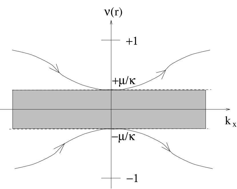
Figure 6: The propagation properties of bending waves are summarized in this diagram. As in the previous figures, $\nu$ represents $\tilde{\omega}/\kappa$. It is a monotonically increasing function of $r$. See text for explanations.

Our motive for the investigation of non-WKB effects is that the dispersion relation of warps is similar in structure to that of spiral waves, with a positive rather than negative self-gravity term. It is thus analogous to the dispersion relation for spiral waves in a disk embedded in a strong vertical magnetic field, as derived by Tagger et al. (1990). They showed that these waves were still subject to a weak form of the Swing amplification mechanism, associated mathematically with the presence of the square root ($q=(k_{x}^{2}+k_{y}^{2})^{1/2}$) in the self-gravity term. Physically, this corresponds to the long-range action of gravity or of magnetic stresses. Thus we can expect the same mechanism to apply to warps.

However this amplification takes place when $k_{x}$ is of the order of $k_{y}$, so that the WKB approximation cannot be used straightforwardly. Although we might use the method of Pellat et al. (1990) for an analytical derivation, we present here a full numerical solution which allows us to derive the result directly. We stay in the shearing sheet and use the formalism developed by various authors (Goldreich and Lynden-Bell, 1965; Toomre, 1964; Drury, 1980; Lin and Thurstans, 1984), reviewed in Tagger et al. (1994), to compute the amplification. We refer to these works for a complete description of the formalism, where one uses the fact that because of the shearing motions $k_{x}$ changes with time as $k_{x}^{0}-2Ak_{y}t$. Thus the $\tilde{\omega}$ term obtained in the WKB approximation, is replaced in the Euler equation by derivatives:

$$\tilde{\omega}\rightarrow\frac{\partial}{\partial t}-2Ak_{y}{\partial\over{\partial k_{x}}}$$

This in turn can be, through a change of variables, transformed to a single derivative over $k_{x}$. There results a set of differential equations which, in the tightly-wound limit ($k_{x}\gg k_{y}$), reduce to the WKB result while at low $k_{x}$ they give rise to transient phenomena and amplification. We write and solve numerically these equations.

At large (positive or negative) $k_{x}$ one recovers the WKB results, while amplification can occur at $k_{x}\sim k_{y}$. The amplification can be described in the following manner: one can combine the equations and find at large $k_{x}$ WKB solutions, varying as

$$M(k_{x})=P^{-1/4}\exp\left(\pm i\int_{0}^{k_{x}}P^{1/2}(k_{x}^{\prime})dk_{x}^{\prime}\right)$$ (13)

where $M$ is any perturbed quantity and $P(k_{x})$ a quantity which appears in equations as the square of an “instantaneous” frequency. These solutions correspond to leading and trailing waves respectively for $k_{x}$ negative or positive, propagating inside or beyond corotation respectively for the + and - signs in the exponent. The leading waves propagate toward corotation, and trailing waves away from it.

Thus let us start at $k_{x}\rightarrow-\infty$ (i.e. leading waves) with a “pure” solution (i.e. with the $+$ sign in the exponent), corresponding to a wave traveling inside and toward corotation. The numerical integration over $k_{x}$ corresponds to following the wave as it approaches corotation, and then is reflected when $k_{x}$ becomes positive. But in the meantime the WKB approximation has lost its validity while $k_{x}\sim k_{y}$, so that the “pure” solution has lost its identity. Thus in general, when the WKB approximation becomes valid again (at large and positive $k_{x}$), we should obtain a mixture of the two solutions, with the $+$ and $-$ sign in the exponent: this means a mixture of trailing waves traveling inside and outside corotation, and away from it: as the initial leading wave is reflected it also “tunnels” through the corotation region, and generates an outgoing trailing wave. This is the usual process of the Swing amplification mechanism for spiral waves; in that case the complex physics of this mechanism implies that the reflected wave has a larger amplitude than the initial one, because waves have negative energy inside corotation and positive energy outside. Thus that by conservation of energy the emission of the positive energy wave outside corotation means an amplification of the negative energy one.

In the case of warps the mechanism is exactly similar; however the repulsive, rather than attractive, force between density perturbations on either side of corotation makes it much less efficient than in the case of spirals: one can obtain an amplification by a hundred in the most extreme case for spirals, while Tagger et al. (1990) find only a factor 1.05 (and a relative amplitude .3 for the transmitted wave) in the best case, when they study magnetized disks with a dispersion relation mathematically similar to that of warps.

Here we obtain similar results, summarized in figures (7) and (8). This amplification is so weak that it is negligible for a single wave packet traveling in the disk. One might consider building a normal mode, formed as in the case of spiral when the reflected trailing wave is reflected back at the galactic center to become a leading one traveling back toward corotation; then, with an amplification by a factor $1.05$, and assuming that the wave suffers no dissipation, the $e$-folding time would be about 20 times the duration of this cycle, which is at best a few rotation times. This means that such modes could not reach a sizable amplitude in a galactic disk over a Hubble time. On the other hand, in accretion disks where the possible number of rotation periods is much larger, and still neglecting all possible sources of dissipation, this might provide a way of maintaining long-lived warp modes.

We wish to note that this result has also been obtained independently by J. Goodman (private communication).

Figure 7: In this figure we show the mean deviation of the warp from the galactic plane, i.e. $\int_{0}^{+\infty}\rho_{0}(z)s(z)dz/(\Sigma/2)$, solved from the full set of differential equations over $k_{x}$. The parameters of the simulation are indicated in the diagram. We have set $4\pi G=1$ and $\Omega=1$. The units in $Z$ are arbitrary, since the perturbation is linear. The vertical profile of $\rho$ is imposed through the use of the consistency equation (9) by the choice of the parameters $a$, $\rho_{m}$ and $A/\Omega$. Here, the high value of $\rho_{m}$ (in our units) and the value of $A/\Omega$ close to $-1/2$ give a disk dominated by the local gravity, i.e. with a vertical profile close to $1/\cosh^{2}(z/H)$. This can be easily checked with the values of the parameters $\mu/\kappa$ and $Q$, which appear to be respectively, in this case, $7.1\times 10^{-2}$ and $0.63$ (just above the stability limit for this type of moderately thick disk). The solid line represents the real part, and the dotted one the imaginary part. For $k_{x}<-k_{y}$, the solution remains WKB, with a decreasing frequency and an increasing amplitude (respectively due to the behavior of $\tilde{\omega}$ with $q$ and to the $P^{-1/4}$ term in the WKB solution). Since we have only one wave propagating in this region, real and imaginary parts are in quadrature. After crossing the region where $k_{x}\sim k_{y}$, the real and imaginary parts are no longer in quadrature, because the solution now projects onto both WKB solutions, and we see that total amplitude has changed.

Figure 8: In this figure we plot the imaginary part of the warp deviation versus its real part, for the same simulation as figure (7). The “trajectory” first follows circles of slowly increasing radius, as the “pure” leading WKB solution travels toward corotation. When $k_{x}$ has become positive, the trajectory becomes elliptic, because the solution is now a mixture of perturbations varying as $\exp\pm i\int P^{1/2}dk_{x}^{\prime}$. The measure of the ellipticity gives the ratio of the transmitted to the reflected wave.

6 Discussion

We have investigated the dispersion relation of warps in a moderately thick disk. We have found that the propagation of warps is described by the dispersion relation (10), with the following hypothesis:

• We work in the shearing sheet model;

• The disk is consistent (with our definition, see the corresponding section), which physically means that the disk must be moderately thick: it is geometrically thin but the ratio of the sound time through the disk to the rotation time is arbitrary;

• The warp wavelength is larger than the disk thickness;

• The disk is isothermal;

• the waves are WKB, i.e. tightly wound.

The corrective term is due to the effect of compressibility, acting when the sound time through the disk is not much smaller than the rotation time.

The associated horizontal motions are important because they allow one to consider the possibility of a non-linear mechanism to continuously excite the warps: indeed the beat wave of two $m=1$ warps (or of a warp with itself) is an $m=2$ perturbation, whose potential and horizontal motion are even in $z$; thus they have the wavenumber and parity of a spiral. This means that a spiral can interact non-linearly with warps and excite them, in the same manner that it can do with other spirals. Non-linear coupling of bars and spirals has been studied by Tagger et al. , 1987, and Sygnet et al. , 1988. This mechanism was found very efficient and explained the behavior of numerical simulations of galactic spiral; in a forthcoming paper we will consider the possibility and the efficiency with which non-linear coupling of warps and spirals might feed warps from the energy and angular momentum carried by the spiral wave to the outer parts of the galactic disk.

Another potentially important effect of the compressional term relates to the possible existence of warp modes, i.e. standing wave structures, in the disk. Classically, the Hunter-Toomre criterion shows that modes can exist only if the integral $\int q\ dr$ is finite, and that with the thin-disk dispersion relation this can be written as $\int dr/\Sigma$ finite - a condition that is difficult to fulfill in realistic disk models. With the new compressional term, this connection between the two integrals disappears, so that one might have $\int q\ dr$ finite (i.e. a discrete mode spectrum) even when $\int dr/\Sigma$ is not bounded.

We have also investigated the self-amplification of $m>1$ warps by a weak form of the SWING mechanism. We have found an amplification which is too weak to significantly amplify warps in galactic disks, but might be considered in accretion disks.

7 Acknowledgments

We wish to thank C. Pichon for rich and helpful discussions in the course of this work. We also thank the referee A. Romeo for very detailed discussions and advice which have considerably enriched this paper.

8 Appendix: derivation of the dispersion relation

We derive hereafter the relation dispersion of warps in the monofluid case under the hypothesis mentioned in the main text.

Let N be:

$$N\equiv\int_{0}^{+\infty}\alpha(z)dz=\int_{0}^{+\infty}\frac{\rho_{0}}{\tilde{\omega}}\biggl{(}a^{2}\frac{\partial s}{\partial z}+\frac{\partial\phi}{\partial z}\biggr{)}dz$$ (14)

where use of equation (6) has been made. Using the unperturbed hydrostatic equilibrium and the expression of $s$ given by equation (5) we rewrite $N$ as:

$$N=-\frac{S}{\tilde{\omega}^{2}}\int_{0}^{+\infty}\frac{\partial\phi_{0}}{\partial z}\frac{\partial\alpha}{\partial z}dz+\frac{1}{\tilde{\omega}}\biggl{(}\frac{a^{2}q^{2}S}{\tilde{\omega}^{2}-\kappa^{2}}+1\biggr{)}\int_{0}^{+\infty}\rho_{0}\frac{\partial\phi}{\partial z}dz$$

where we have defined

$$S=\frac{\tilde{\omega}^{2}-\kappa^{2}}{\tilde{\omega}^{2}-\kappa^{2}-a^{2}q^{2}}$$ (15)

The $a^{2}q^{2}$ term in the denominator is the source of the new effect we introduce. It clearly represents the effect on $s$ of the compressibility associated with the horizontal motions.

Integrating by parts the first term, we use the Poisson equation and the consistency hypothesis (i.e. that $\Delta_{r}\phi_{0}$ does not depend on $z$), and get:

$$N=\frac{4\pi GS}{\tilde{\omega}^{2}}\int_{0}^{+\infty}\rho_{0}\alpha dz-\frac{S\Delta_{r}\phi_{0}}{\tilde{\omega}^{2}}N+\frac{S}{\tilde{\omega}}\int_{0}^{+\infty}\rho_{0}\frac{\partial\phi}{\partial z}dz$$ (16)

Where we have made use of the parity properties of the warp ($s=0$ and $\phi=0$ at $z=0$).

We see here that the consistency hypothesis is the key to our derivation, since it has allowed us to extract $\Delta_{r}\phi_{0}$ from the integral, in the second term of the right-hand side.

We write the solution of the Poisson equation (Equation 7) as:

$$\phi=-e^{qz}\int_{z}^{+\infty}\frac{4\pi G\rho_{0}(z^{\prime})s(z^{\prime})}{2q}e^{-qz^{\prime}}dz^{\prime}$$

$$-e^{-qz}\int_{-\infty}^{z}\frac{4\pi G\rho_{0}(z^{\prime})s(z^{\prime})}{2q}e^{qz^{\prime}}dz^{\prime}$$

(one easily checks that this is the solution which verifies the boundary conditions at $z=0$ and at $z\rightarrow\infty$).

Since $\rho_{0}$ vanishes beyond a vertical scale $H$ we can expand the exponential to first order in $qH$; this gives, after straightforward computations using the continuity equation (5):

$$\int_{0}^{+\infty}\rho_{0}\frac{\partial\phi}{\partial z}dz=-\frac{4\pi G}{\tilde{\omega}}\int_{0}^{+\infty}\!\rho_{0}\alpha dz+$$

$$\frac{4\pi Gq}{\tilde{\omega}}\int_{0}^{+\infty}\!\rho_{0}(z)dz\int_{0}^{+\infty}\!\!\alpha dz+O_{grav}[(qH)^{2}]$$

where $O_{grav}[(qH)^{2}]$ means that this gravitational contribution also contains a term of second order in $qH$ which we have not evaluated, truncating the expansion of the exponentials to first order. An analytical computation of this can be performed if one assumes that the motion in the warp is vertical with a vanishing divergence, and if one has an analytical expression (e.g. a gaussian) for the vertical equilibrium density profile. In these conditions one finds that the dispersion relation is modified by replacing the surface density $\Sigma$ by an apparent surface density $\Sigma^{\prime}=\Sigma(1-\lambda qH)$, where $\lambda$ is a constant equal to $(2\pi)^{-1/2}$ in the gaussian case. Thus this term affects the dispersion relation only in the limit $qH\sim 1$, whereas the compressional term we have derived can play a role for an arbitrarily small value of $qH$. The computation of this gravity term could be well approximated by the use of “softened gravity” models (Erikson 1974, Athanassoula 1984, Romeo 1994) where one artificially truncates the $(r-r^{\prime})^{-1}$ divergence of the potential to take into account the geometric effect of the finite disk thickness. Thus hereafter we neglect this second-order gravitational term.

Substituting our result and the value of $S$ in equation (16), and dividing by $N$, we find the dispersion relation:

$$\tilde{\omega}^{2}=-\Delta_{r}\phi_{0}+2\pi G\Sigma q+\frac{\tilde{\omega}^{2}}{\tilde{\omega}^{2}-\kappa^{2}}a^{2}q^{2}+O_{grav}[(qH)^{2}].$$

References

- (1) Athanassoula, E., 1984, Phys. Rep. 114, 319
- (2) Bertin, G., and Casertano, S., 1982, A&A 106, 274
- (3) Bertin, G., and Mark, J. W.-K., 1980, A&A 88, 289
- (4) Binney, J., 1992, ARA&A 30, 51
- (5) Binney, J. and Tremaine, S., 1987, Galactic Dynamics, pp. 406 to 416, Princeton University Press
- (6) Drury, L. O’C., 1980, MNRAS 193 337
- (7) Dubinski, J. and Kuijken, K., 1995, ApJ 442, 492
- (8) Erikson, 1974, Ph.D. Thesis, MIT
- (9) Florido, E., Battaner, E., Prieto, M., Mediavilla, E., and Sanchez-Saavedra, M.L., 1991, MNRAS 251, 193
- (10) Goldreich, P., and Lynden-Bell, D., 1965, MNRAS 130, 125
- (11) Hunter, C., and Toomre, A., 1969, ApJ 155, 747
- (12) Lin, C.C. and Thurstans, R.P., 1984, in Proc. of a course on Plasma Astrophysics, Varenna, Italy, ESA S.P. 207 (Noordwijk, Holland), 121
- (13) Nelson, A.H., 1976, MNRAS 177, 265
- (14) Nelson, A.H., 1981, MNRAS 196, 557
- (15) Papaloizou, J.C.B., Lin, D.N.C., 1995, ApJ 438, 841
- (16) Pellat, R., Tagger, M., Sygnet, J.F., 1990, A&A 231, 347
- (17) Quiroga, R.J., Schlosser, W., 1977, A&A 57, 455
- (18) Romeo, A.B., 1992, MNRAS 256, 307
- (19) Romeo, A.B., 1994, A.&A 286, 799
- (20) Shu, F.H., 1968, Ph.D. thesis, Harvard University.
- (21) Sparke, L.S., 1984, ApJ 280, 117
- (22) Sparke, L.S., Casertano, S., 1988, MNRAS 234, 873
- (23) Sygnet, J.F., Tagger, M., Athanassoula, E., Pellat, R., 1988, MNRAS 232, 733
- (24) Tagger, M., Sygnet, J.F., Athanassoula, E., Pellat, R., 1987, ApJ 318, L43
- (25) Tagger M., Henriksen, R.N., Sygnet, J.-F., Pellat R., 1990, ApJ 353, 654
- (26) Tagger, M., Sygnet, J.-F., Pellat, R., 1994, in N-body problems and gravitational dynamics, proceedings of a Meeting held in Aussois, F. Combes and E. Athanassoula ed., p. 55
- (27) Terquem, C., 1993, Ph.D. Thesis, Université Joseph Fourier de Grenoble
- (28) Toomre, A., 1964, ApJ 139, 1217
- (29) Toomre, A., 1966, in Proceedings of a summer study program in Geophysical Fluid Dynamics, Woods Hole Oceanographic Institution, 1966
- (30) Toomre, A., 1983, in Internal Kinematics and Dynamics of Galaxies, IAU Symp. 100, E. Athanassoula ed., 177
- (31) Vandervoort, P.O., 1970, ApJ 161, 87