Reconstruction of cosmological initial conditions from galaxy redshift catalogues

Abstract

We present and test a new method for the reconstruction of cosmological initial conditions from a full-sky galaxy catalogue. This method, called ZTRACE, is based on a self-consistent solution of the growing mode of gravitational instabilities according to the Zel’dovich approximation and higher order in Lagrangian perturbation theory. Given the evolved redshift-space density field, smoothed on some scale, ZTRACE finds via an iterative procedure, an approximation to the initial density field for any given set of cosmological parameters; real-space densities and peculiar velocities are also reconstructed. The method is tested by applying it to N-body simulations of an Einstein-de Sitter and an open cold dark matter universe. It is shown that errors in the estimate of the density contrast dominate the noise of the reconstruction. As a consequence, the reconstruction of real space density and peculiar velocity fields using non-linear algorithms is little improved over those based on linear theory. The use of a mass-preserving adaptive smoothing, equivalent to a smoothing in Lagrangian space, allows an unbiased (although noisy) reconstruction of initial conditions, as long as the (linearly extrapolated) density contrast does not exceed unity. The probability distribution function of the initial conditions is recovered to high precision, even for Gaussian smoothing scales of $\sim 5$ $h^{-1}\;{\rm Mpc}$, except for the tail at $\delta\geq 1$. This result is insensitive to the assumptions of the background cosmology.

1 Introduction

Large and homogeneous galaxy catalogues are defining the present-day density field of galaxies to increasing precision. Assuming that galaxies trace the underlying matter field in some known way, it should be possible to trace the matter density field back in time, thus recovering the initial conditions of the local Universe. The initial conditions are of importance for at least two reasons: firstly, it is interesting to examine the probability distribution function (hereafter PDF) of the initial density field, which is expected to be Gaussian in many theories of the origin of fluctuations (see e.g. Linde, 1990); secondly, it is possible to use the initial conditions derived from a galaxy redshift survey as the starting point for an N-body simulation, to reproduce the non-linear dynamics of our local Universe in some detail (see, for example, Kolatt et al. 1996).

Although conceptually simple, the implementation of this idea to real data presents some difficulties. Firstly, it is not possible to integrate the present-day density field back in time with an N-body simulation: the familiar decaying mode of cosmological matter perturbations will amplify noise in the backward integration. This can be avoided by using semi-analytical methods restricted to pure growing-mode dynamics (see Nusser & Dekel 1992). Secondly, the galaxy density field is measured in redshift space; this complicates the analysis as redshift space is not isotropic, except around the observer, and the map from initial to final positions is not irrotational (see Section 2). Moreover, “multi-stream” regions around collapsing structures affect the mapping from the initial conditions to both the real and redshift space galaxy distribution. In redshift space, multi-stream regions are sometimes referred to as “triple valued” regions. The existence of multi-stream regions imposes a fundamental limit on the accuracy of reconstruction algorithms. In Section 2 we show that the effect of multi-streaming is more severe in redshift space than in real space. Thus the reconstruction of density fields using redshift surveys is limited to modest (real-space) density contrasts ($\delta\rho/\rho\la 1$). Thirdly, the galaxy density field is generally estimated from flux limited galaxy catalogues, which become sparse at large distances; it will be shown in Section 4 that the density estimate provides an important source of noise in the reconstruction of initial density fields. Fourthly and most importantly, the relationship between galaxies and the underlying mass density distribution is not well known. Thus progress can only be made if we adopt simple assumptions concerning the nature of this relationship.

The most widely used analytical tool for the evolution of large-scale structure is linear perturbation theory. The topic of redshift-space distortion in linear theory has been reviewed by Hamilton (1998). Linear theory has been used to recover the real-space density and peculiar velocity fields from near all-sky galaxy catalogues, for example, the QDOT (Kaiser et al. 1991), 1.2 Jy (Yahil et al. 1991; Webster, Lahav & Fisher 1997) and PSCz (Branchini et al. 1998) IRAS catalogues, the optical catalogue compiled by Hudson (1994), the Optical Redshift Catalogue (ORS; Baker et al. 1998), and the Abell clusters catalogue (Branchini & Plionis 1996). On the other hand, linear theory cannot be used to recover the initial conditions of our local Universe. According to linear theory, the initial density field is just a rescaled version of the final one (in real space), which is strongly non-Gaussian as long as the mass variance is not much less than unity.

The Zel’dovich (1970) approximation offers a useful tool for reconstructing initial conditions, as it provides a description of the growing mode of gravitational evolution in the mildly non-linear regime when the variance of the density field is of order unity. Nusser & Dekel (1992) recast the Zel’dovich approximation in terms of a Bernoulli-type evolution equation for the peculiar velocity potential which can easily be integrated back in time once the present-day peculiar velocity field is known. In fact, another reconstruction algorithm is needed to obtain the peculiar velocity potential. Nusser, Dekel & Yahil (1995) applied the formalism of Nusser & Dekel (1992) to the peculiar velocity potential found by applying a non-linear approximation to the IRAS 1.2 Jy catalogue (see also Yahil et al. 1991). They found that the initial conditions of the local Universe (smoothed with a Gaussian filter of width 10 $h^{-1}\;{\rm Mpc}$) are consistent with a Gaussian PDF for simple models of the relative bias between the galaxy and mass distributions. An alternative, improved method, which is consistent with mass conservation, is given by Gramann (1993a). Gramann (1993b) and Susperregi & Buchert (1997) extended the formalism to second order in the Lagrangian perturbation theory. Taylor & Rowan-Robinson (1993) developed a quasi-non-linear reconstruction algorithm in which the dynamics is still described at a linear level, but the mapping from real- to redshift-space is solved exactly.

A simpler method was proposed by Weinberg (1992). If the PDF of initial conditions is assumed to be Gaussian, then a better estimate of the initial conditions is obtained by “Gaussianizing” the PDF computed using linear theory. Assuming that non-linear dynamics preserves the order of densities, the inferred initial densities can be rescaled by an order-preserving transformation so that they have a Gaussian PDF. Methods of this kind were used by Kolatt et al. (1996) and by Narayanan & Weinberg (1998), where the Gaussianization procedure was applied to the results of a Zel’dovich reconstruction. The obvious problem with this method is that the Gaussianity of the PDF is assumed instead of being inferred from the data. For example, the initial PDF of the galaxy distribution may well not be Gaussian if the relation between the galaxies and the mass distribution is complex. Moreover, the order-preserving condition may be a poor approximation of the actual dynamics because of the non-locality of gravitational evolution.

A different approach based on least action was proposed by Peebles (1989, 1990). The initial positions of galaxies in a catalogue can be found by searching for the displacements which satisfy a least action constraint under some assumption regarding the mass distribution (e.g that all of the mass is associated with point-like galaxies). A version of this method was tested by Branchini & Carlberg (1994) who found that it can lead to an underestimate of the cosmological density $\Omega$, and applied to the groups of the local supercluster by Shaya, Peebles & Tully (1995). Actually, as shown by Giavalisco et al. (1993) and Croft & Gatzañaga (1997), the Zel’dovich approximation is the first-order solution of the least-action principle. Croft & Gatzañaga (1997) used the least action principle to set up a reconstruction method based on the Zel’dovich approximation, called path-interchange Zel’dovich approximation (hereafter PIZA). Given a set of points coming from a uniform configuration, the map from initial to final positions is found by minimizing the action constructed by the average square displacement. Although different from the other reconstruction algorithms, the least-action methods suffer from similar problems to the methods described above: the mapping from redshift- to real-space presents similar difficulties, multi-streaming gives multiple solutions for the orbits, and some specific assumption (analogous to bias) is required to relate the mass and galaxy distributions.

Narayanan & Croft (1998) compared the performances of different reconstruction algorithms to N-body simulations. The most accurate initial conditions were recovered by the hybrid reconstruction scheme of Narayanan & Weinberg (1998) and by the PIZA scheme. However, in their tests the initial conditions were reconstructed from the full output of the simulation in real space and the effects of redshift-space distortions and of the galaxy selection function, critical in the analysis of real galaxy catalogues, were ignored.

The Zel’dovich approximation can be used to obtain the initial density field directly from the redshift-space density field, under some assumption of bias. This cannot be achieved with the Bernoulli equation of Nusser & Dekel (1992) or with the alternative one of Gramann (1993a), as they require as input the peculiar velocity potential, which is obtained (in a way that is not self-consistent) from a linear theory analysis. The PIZA method is in principle able to give a self-consistent determination of initial condition.

The approaches of Nusser & Dekel (1992) and Gramann (1993a) cannot be extended beyond the Zel’dovich approximation without major changes to the formalism (see Gramann 1993b; Susperregi & Buchert 1997). It is well known that the Zel’dovich approximation is the first term of a Taylor expansion of the Lagrangian map (see, e.g., Moutarde et al. 1991; Buchert & Ehlers 1993; Catelan 1995), and it would be desirable to develop a reconstruction analysis that is easily extendible to higher orders to check whether or not such contributions are important. The effects of higher order terms have been analyzed, for instance, by Gramann (1993b), Hivon et al. (1995) and Chodorowsky et al. (1998).

In this paper we present an iterative reconstruction algorithm based on a self-consistent solution of the Zel’dovich (or higher-order) approximation; this algorithm is able to find the initial density field which evolves, with Zel’dovich (or 2nd-order Lagrangian perturbation theory), into a given final density field in redshift space. In addition to the initial conditions, the real-space density field and the line-of-sight (hereafter LOS) peculiar velocity field can be recovered. Here, we focus on the recovery of initial conditions because, as will be shown in Section 5, when applied to realistic simulated galaxy catalogues non-linear reconstruction algorithms do not give greatly improved final density and velocity fields over those inferred using linear theory (which is, of course, much easier to implement).

The paper is organized as follows: Section 2 presents the mathematical formalism and describes the iterative method. Section 3 describes the numerical simulations used to test the reconstruction algorithms. In Section 4 we describe the noise introduced by estimating the density from a catalogue of discrete points. The results of the reconstruction algorithm and tests against N-body simulations are presented in Section 5. The conclusions are summarized in Section 6.

Throughout this paper all distances are given in $h^{-1}\;{\rm Mpc}$, with $h=H_{0}/(100\ km/s/Mpc)$.

2 The Reconstruction Algorithm

2.1 Equations

The evolution of a self-gravitating fluid can be described by Lagrangian fluid-dynamics. In this approach, the dynamical variable is the displacement ${\bf S}$, which maps the point-mass particles from the initial (comoving Lagrangian, ${\bf q}$) to the final (comoving Eulerian, ${\bf x}$) position:

$${\bf x}({\bf q},t)={\bf q}+{\bf S}({\bf q},t).$$ (1)

The Euler-Poisson system of equations (see Peebles 1980) can be recast in terms of a set of equations for the displacement ${\bf S}$; these equations are given by Buchert (1989), Bouchet et al. (1995) and Catelan (1995). The notation used in this paper follows that of Catelan (1995). The system can be solved perturbatively for small displacements. Denoting by $D(t)$ the linear growing mode, the first two terms of the perturbative series are:

$${\bf S}^{(1)}({\bf q})=-D(t)\nabla\varphi({\bf q});$$ (2)

$${\bf S}^{(2)}({\bf q})=-\frac{3}{14}D(t)^{2}\nabla\varphi^{(2)}({\bf q}).$$ (3)

$\varphi({\bf q})$ is simply a rescaled version of the initial peculiar gravitational potential, such that:

$$\nabla^{2}\varphi({\bf q})=\delta({\bf q},t_{i})/D(t_{i}),$$ (4)

where $\delta(t_{i})$ is the initial density contrast ($\delta=(\varrho-\bar{\varrho})/\bar{\varrho}$), and $D(t_{i})$ is the growing mode at the initial time $t_{i}$. Note that the quantity $\delta_{l}({\bf q})=\delta({\bf q},t)/D(t)$ is constant in linear theory. If the growing mode is normalized to $D(t_{0})=1$ at the final time $t_{0}$, $\delta_{l}$ is the density contrast linearly extrapolated at $t=t_{0}$; this quantity will be referred to as the linear density contrast in this paper. Note also that the map ${\bf S}$ has been assumed to be irrotational because rotational components do not contribute to the growing mode.

The second-order potential obeys another Poisson equation:

$$\nabla^{2}\varphi^{(2)}({\bf q})=2\mu_{2}(\varphi_{,ab}),$$ (5)

where $\mu_{2}(\varphi_{,ab})=(\varphi_{,aa}\varphi_{,bb}-\varphi_{,ab}\varphi_{,ab})/2$ is the second principal invariant of the tensor of second derivatives of $\varphi$ (comma denotes derivative with respect to the Lagrangian coordinate ${\bf q}$, summation over repeated indices is assumed; see, e.g., Catelan 1995).

The peculiar velocity ${\bf v}$ of the mass element ${\bf q}$ is obtained from the displacement ${\bf S}$ as:

$${\bf v}({\bf q},t)=a\frac{dD}{dt}\frac{d{\bf S}}{dD}=\frac{dD}{dt}\frac{a}{D}({\bf S}^{(1)}+2{\bf S}^{(2)}+\ldots).$$ (6)

Here $a(t)$ is the scale factor (normalized to $a(t_{0})=1$). In a reference frame centred on the observer, the redshift-space coordinate ${\bf s}$ is defined as:

$${\bf s}({\bf q},t)={\bf x}({\bf q},t)+\frac{1}{aH}({\bf v}({\bf q},t)\cdot\hat{{\bf x}}({\bf q},t))\hat{{\bf x}}({\bf q},t).$$ (7)

Here $H(t)$ is the Hubble parameter, while $\hat{{\bf x}}$ is the versor of ${\bf x}$. It is possible to define a redshift-space map ${\bf S}^{(s)}$ as follows:

$${\bf s}({\bf q},t)={\bf q}+{\bf S}^{(s)}({\bf q},t).$$ (8)

Then:

$${\bf S}^{(s)}({\bf q},t)=$$

$${\bf S}^{(1)}+{\bf S}^{(2)}+\ldots+f(\Omega)[({\bf S}^{(1)}+2{\bf S}^{(2)}+\ldots)\cdot\hat{{\bf x}}]\hat{{\bf x}}.$$

The function $f(\Omega)=d\ln D/d\ln a$ is usually approximated by $f(\Omega)\simeq\Omega^{0.6}$ (Peebles 1980); if a cosmological term is present, then $f(\Omega,\Omega_{\Lambda})\simeq\Omega^{0.6}+\Omega_{\Lambda}(1+\Omega/2)/70$ (Lahav et al. 1991). It is noteworthy that, while the real-space map ${\bf S}$ is irrotational, the redshift-space one ${\bf S}^{(s)}$ is in general rotational (see, e.g., Nusser & Davis 1994).

Given a map ${\bf S}$, the density contrast can be calculated through the continuity equation:

$$1+\delta({\bf q})=\frac{1}{\det(\delta^{K}_{ab}+S_{a,b})}.$$ (10)

Here $\delta^{K}_{ab}$ is the Kronecker tensor. It is useful to recall the identity:

$$\det(\delta^{K}_{ab}+S_{a,b})=1+\mu_{1}({\bf S})+\mu_{2}({\bf S})+\mu_{3}({\bf S}),$$ (11)

where $\mu_{i}({\bf S})$ are the principal invariants of the first derivative tensor of S; $\mu_{1}=S_{a,a}$ is the divergence of the displacement ${\bf S}$, $\mu_{2}({\bf S})=(S_{a,a}S_{b,b}-S_{a,b}S_{a,b})/2$, and $\mu_{3}({\bf S})=\det(S_{a,b})$.

Inserting the redshift-space map ${\bf S}^{(s)}$ (Eq. 2.1) into Eq. 10, and noting that $\mu_{1}({\bf S}^{(1)})=-D\delta_{l}$ (Eqs. 2 and 4), the following identity is obtained:

$$\delta_{l}=$$

$$\frac{1}{D}\left[\frac{\delta_{s}}{1+\delta_{s}}-\mu_{1}({\bf S}^{(1)})+\mu_{1}({\bf S}^{(s)})+\mu_{2}({\bf S}^{(s)})+\mu_{3}({\bf S}^{(s)})\right].$$

Here $\delta_{s}$ is the density contrast in redshift space, to be distinguished from the real-space density contrast $\delta_{x}$.

The perturbative series breaks down when the map in Eq. 1 or Eq. 8 becomes multi-valued. For the real-space map, when this takes place the interested mass elements undergo pancake collapse and go into the multi-stream regime. On the other hand, redshift-space multi-streaming takes place when a perturbation decouples from the Hubble flow; the infall velocity then becomes comparable to the difference in redshift across the collapsing region and the distance-redshift relation becomes triple-valued. The perturbative expansion will thus break down at lower real-space density contrasts when applied to redshift space.

The linear theory limit can be derived easily from the equations presented above. Displacements are assumed to be infinitesimally small, and the displacement from ${\bf q}$- to ${\bf x}$-space gives only a second-order contribution to the density, so that the difference between Eulerian and Lagrangian spaces can be neglected. The real-space density contrast is simply:

$$\delta_{x}=-\frac{\nabla\cdot{\bf v}}{aHf(\Omega)},$$ (13)

while the redshift-space density is:

$$\delta_{s}=\delta_{x}+Df(\Omega)\nabla\cdot[(\nabla\varphi\cdot\hat{{\bf x}})\hat{{\bf x}}].$$ (14)

2.2 The Method: Iteration and Convergence

Given a smooth evolved density field evaluated on a regular grid in redshift space, we want to obtain the linear density field $\delta_{l}$ which evolves into the input density field. A direct inversion of the equations presented in the previous section is intractable; however, the identity given in Eq. 2.1 can be used to set up an iterative method to reconstruct the initial conditions $\delta_{l}$. The first guess for the linear density contrast can be simply given by $\delta_{s}/(1+\delta_{s})$, where $\delta_{s}$ is the evolved redshift-space density contrast; from the first guess initial density it is possible to obtain numerically the map S in real and redshift space from Eqs 4, 2 and 3, and then, using Eq. 2.1, a new guess for the linear density can be found. This cycle can be repeated until convergence is achieved.

The input redshift-space density field must be smoothed to eliminate high density contrasts and regions of orbit-crossing, where we would not expect the reconstruction method to work.

The final density field $\delta_{s}$ is given on a regular grid in redshift ${\bf s}$-space, while the reconstruction is performed on a regular grid in the Lagrangian ${\bf q}$-space; in other words, the quantity $\delta_{s}$ in Eq. 2.1 is a function of ${\bf q}$, while the input redshift-space field is given as a function of ${\bf s}$. If the map ${\bf S}^{(s)}({\bf q})$ is known (again on the regular grid in ${\bf q}$), one can obtain the ${\bf q}$-space density from the ${\bf s}$-space density by interpolating the density contrast $\delta_{s}$ at the positions in ${\bf s}$-space corresponding to the regular grid in ${\bf q}$-space. The term $\delta_{s}({\bf q})/(1+\delta_{s}({\bf q}))$ in Eq. 2.1 is then, in practice, a function of ${\bf S}$, which changes at each iteration.

The first guess for the map is ${\bf S}=0$, i.e. it is assumed that the ${\bf q}$-space linear density is just given by the ${\bf s}$-space evolved density. As a consequence, the first guess for the linear density is not properly normalized. In fact, the correct normalization of the density field is never guaranteed, as the galaxy catalogue to which the reconstruction algorithm is applied may not be a fair sample of the Universe.

In summary, the iteration method has been implemented as follows:

1. The final, observed density field in redshift space, $\delta_{s}$, is calculated on a cubic grid of points and provided as an input.

2. The first guess for the linear density is just $\delta_{l}({\bf q})=\delta_{s}({\bf s})/(1+\delta_{s}({\bf s}))$, with ${\bf S}^{(s)}=0$ (note that $D(t_{0})=1$: the initial density is just a simple function of the final density.

3. The estimate of the linear density $\delta_{l}$ is used to calculate the peculiar potential $\varphi$ (Eq. 4), the ${\bf x}$-space map ${\bf S}$ (Eq. 2, and Eqs. 5 and 3 if 2nd order is used), the peculiar velocity ${\bf v}$ (Eq. 6) and the ${\bf s}$-space map ${\bf S}^{(s)}$ (Eq. 2.1).

4. Eq. 2.1 is used to obtain a new guess for the linear density $\delta_{l}$.

5. Steps (iii) and (iv) are repeated until the mean square difference between the old and new estimates of the linear density field meets a specified criterion and the density field is convergent at each grid point.

Differentiation and the solution of the Poisson equations are done with Fast Fourier Transforms (FFTs): FFTs provide fast and accurate derivatives of the density and velocity fields. However, periodic boundary conditions do not hold in redshift space. The natural geometry of an all-sky galaxy catalogue is spherical, and the imposition of periodic boundary conditions is clearly artificial. Periodic boundary conditions are forced by padding the density field outside the largest sphere inscribed within the cubic volume used for the FFT. The padding value is chosen so that the initial density field has zero mean within the whole box; this procedure defines the overall normalization of the density field at each iteration.

The iteration scheme is used to solve a complex non-linear and non-local set of equations. The convergence of the iterative method is not guaranteed and care is needed to achieve it. The occurrence of orbit crossing at a few points may indicate some problem with the convergence, but Eq. 2.1 forces the system into the single-stream regime, so it is possible to recover from orbit crossings in many cases. The most problematic points are (perhaps counterintuitively at first sight) not large overdensities, but deep underdensities; the final density $\delta_{s}$ enters Eq. 2.1 as $\delta_{s}/(1+\delta_{s})$, so the contribution from overdensities asymptotically approaches unity. Deep underdensities, however, give large negative contributions (moreover, as shown by Sahni & Shandarin 1996 and Monaco 1997, the perturbative Lagrangian series does not even converge in deep underdensities). Another problem with the convergence is that there are discontinuities at the border of the padded region, especially when no selection function is applied to the density field. Both deep underdensities and discontinuities can make the solution “explode” at some points and this, because of the non-locality of the system of equations, propagates over the whole volume. Finally, the system does not converge at the position of the observer, which is a singular point in the ${\bf x}$–${\bf s}$ tranformation.

The following techniques have been used to help achieve convergence:

1. To avoid oscillations of the solution, at each iteration the new guess for the linear density is given by a weighted mean of Eq. 2.1 and the old guess. This is equivalent to introducing a numerical viscosity for damping the oscillations. The first “old” guess is assumed to be a null field. The weights $w1$ (for Eq. 2.1) and $w2=1-w1$ (for the old guess) are set to 0.2 and 0.8 at the starting time, so that the variance of the first guess is small and no orbit crossing occurs from the start. The weights are increased so as to take values 0.4 and 0.6 after 6 iterations.

2. To force the convergence at the center, both the guess for the density field and the LOS peculiar velocity are smoothed with a filter, $exp(-(q_{cut}/q)^{2})$. As a consequence, the initial density within the central $\sim 2q_{cut}$ grid points is not correctly recovered.

3. To avoid problems due to discontinuities at the border of the padded region, the guess for the linear density is linearly suppressed (i.e. multiplied by a function linearly decreasing with radius) from a given radius up to the padding radius (half the box size). The suppression, which is performed to smoothly join the field with the constant padding value, depends on the padding value itself. In turn the padding value depends on the average value of the field inside the sphere, and hence on the suppression. The padding value is thus found iteratively and usually 3 iterations are sufficient to reach convergence. The distance at which the suppression starts depends on whether a selection function is applied to the density: if we apply the method to the full density field from a numerical simulation, then the density is suppressed from 0.7 times half the box length; if a simulated galaxy redshift survey is used, with the smoothing strategy described in Section 5.2, the outer more sparsely sampled regions are smoother than the inner regions and the suppression can be applied at a radius of 0.9 times half the box length.

4. The deepest underdensities are truncated to a fixed limiting value, set to $\delta_{s}/(1+\delta_{s})=-5$ ($\delta_{s}=-0.83$) with Zel’dovich and $-3$ with 2nd order ($\delta_{s}=-0.75$). This does not have a significant impact on the final results, as just a few grid points are affected by the truncation. On the other hand, such points can make the solution explode.

The linear density is reliably reconstructed only in the central parts of the computational volume. This is a consequence of using an FFT and a Cartesian grid for a problem with a more natural spherical symmetry. However, FFTs allow us to solve the complex system of equations in an acceptable amount of computer time. In principle, we could use spherical harmonics in place of FFTs, but at the cost of a great increase in the complexity of the equations and computer time. It is worth noting that the the non-iterative method of Fisher et al (1995), based on spherical harmonics, can be used only in linear theory when the displacements from the ${\bf q}$- to the ${\bf x}$-space are neglected; the transverse components of such displacements couple different spherical harmonics and a direct inversion of the coupling matrix rapidly becomes computationally intractable as the number of spherical harmonics is increased.

We applied the iterative method to numerical simulations of cold dark matter (CDM) models with a computational box length of 240 $h^{-1}\;{\rm Mpc}$. The models are described more fully in Section 3. Typically, we used a grid of $64^{3}$ points to define the density and velocity fields, thus the grid spacing is 3.75 $h^{-1}\;{\rm Mpc}$. For a smooth density field with variance in the range from 0.1 to 0.7, the iteration method is able to converge in 10-15 iterations; for a $64^{3}$ grid, convergence is achieved in about 5 minutes of CPU time on a DEC Alpha 4100 5/300. The solution is assumed to have converged when the mean square difference between the old and new linear field is smaller than 1% of its variance; we have always checked that the largest difference, which can be comparable to the variance of the field, is decreasing at the convergence. The convergence is slowest in overdensities, so that the height of the highest peaks can be underestimated; on the other hand, those peaks are presumably in multi-stream regime (or in triple-valued regions), so they would be underestimated in any case. The variance of the inferred linear field converges to a stable value.

The method described in this Section will be referred to as ZTRACE in the rest of this paper.

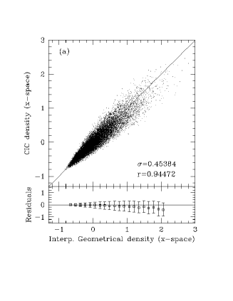
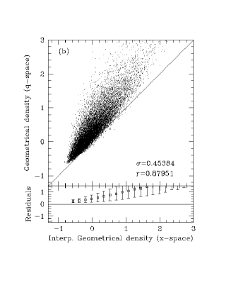
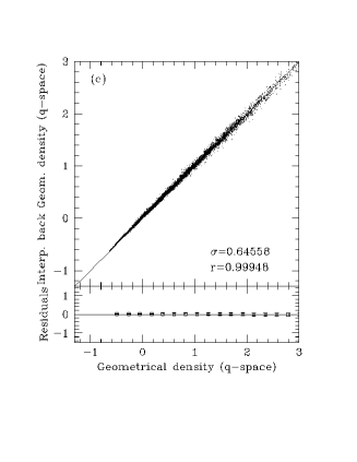
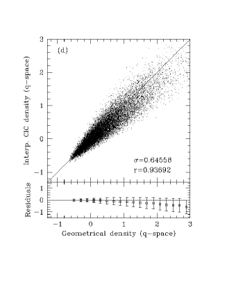
Figure 1: Comparison of the geometrical and CIC density estimates: (a) in ${\bf x}$-space; (b) geometrical density in ${\bf q}$- and ${\bf x}$-space; (c) error introduced by the double interpolation (${\bf q}$-space); (d) error introduced by the CIC estimate (${\bf q}$-space).

The same method has been adapted to two simpler cases, that of linear theory and that in which the real-space density field is given as input. The implementation of linear theory requires minor changes to the method: Eqs. 13 and 14 are used to obtain an estimate of the linear density from the redshift-space density field, while Eq. 6 (obviously with only the first order term) is used to obtain the peculiar velocity. The map from ${\bf q}$- to ${\bf x}$-space has only a formal meaning, as the difference between the two spaces is neglected (at first order in the density). The padding procedure is left unchanged, no limit is set to underdensities, the central smoothing of the field is not performed and the weights $w1$ and $w2$ are set to (0.3,0.7) at the start, increasing to (0.5,0.5) after three iterations. The convergence is reached within 5 iterations. This linear version of the reconstruction method will be referred to as LTRACE.

To compare with the results of Narayanan & Croft (1998), the method has been adapted to recover initial conditions from the real-space density field of a numerical simulation. In this case, periodic boundary conditions hold and neither the padding procedure not the central smoothing are required. The truncation of deep underdensities is still performed, and the weights $w1$ and $w2$ are fixed to (0.5,0.5). The convergence is faster than the application to redshift-space and is achieved in 8-10 iterations. This version will be referred to as XTRACE.

3 N-body Simulations

To test the reconstruction methods we have run N-body simulations with version 2.0 of the Hydra code using pure dark matter (see Couchman, Thomas & Pearce 1995 for full details). $128^{3}$ particles are simulated in a box of length 240 $h^{-1}\;{\rm Mpc}$ using a $256^{3}$ base mesh with adaptive refinements. Two simulations have been run: one in an Einstein-de Sitter (henceforth EdS) Universe with $h=0.5$, and one in an open Universe with $\Omega=0.3$, $h=0.7$ and no cosmological constant. The two simulations have been run with the same random number seed, so that they have the same phases. To generate the initial power spectra, we used the parameterization of Efstathiou, Bond & White (1992) for the power spectrum of an initially scale invariant, adiabatic, CDM-dominated universe. For the power spectrum shape parameter $\Gamma$, we adopted values of $\Gamma=0.5$ for the EdS simulation and $\Gamma=0.21$ for the open simulation. In both simulations the final dispersion of the mass fluctuations within spheres of radius 8 $h^{-1}\;{\rm Mpc}$ was set to $\sigma_{8}=0.7$.

The box length has been chosen so that the radius of the largest sphere contained within the box is 120 $h^{-1}\;{\rm Mpc}$, so that we can reliably simulate a galaxy catalogue out to at least 80 $h^{-1}\;{\rm Mpc}$while having the mass resolution to resolve non-linear structures. The tests of the reconstruction algorithms using the EdS and open simulations are almost identical and so with the exception of Section 5.6, we present comparisons exclusively with the EdS simulation.

4 Noise in Density Estimates

The largest source of noise in the reconstruction algorithms comes from noise in the estimate of the input evolved density field. This can be demonstrated by using a true density field that is given by Eq. 10 from a known displacement map ${\bf S}$, which is in the single-stream regime at all points. The map we use here was generated on a $64^{3}$ grid by applying XTRACE to the output of the Einstein-de Sitter simulation described in the previous section. Even though the displacement is from the ${\bf q}$- to the ${\bf x}$-space, all the conclusions of this Section are valid for ${\bf s}$-space.

The true density, which will be called the geometrical density in this paper, is found with Eq. 10 in Lagrangian space. The corresponding Eulerian-space density can be obtained in two ways: first, one can find by interpolation the ${\bf q}$-grid which according to the map ${\bf S}$ corresponds to a regular grid in ${\bf x}$-space (we use a linear interpolation for this step); the ${\bf x}$-space density can then be found by interpolating the geometrical density at the ${\bf q}$-points corresponding to the ${\bf x}$-space grid (we use a quadratic interpolation for this step).

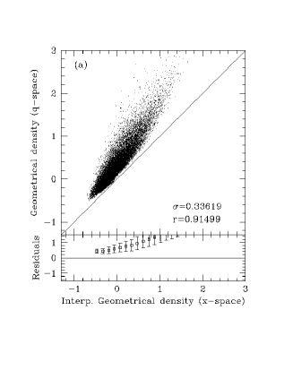
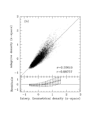
Figure 2: (a) Geometrical density in ${\bf x}$- and ${\bf q}$-space, smoothed over 1.64 grid points (6.15 $h^{-1}\;{\rm Mpc}$), so that 10 particles in the simulated catalogue lie within the Gaussian filter radius on average. (b) and (c) show adaptive and non-adaptive smoothed density estimates of the simulated catalogue compared with the smoothed geometrical density (in ${\bf x}$-space).

The second way of determining the ${\bf x}$-space density, which is valid even if the map is not in the single-stream regime, is to perform a standard cloud-in-cell (hereafter CIC) or similar interpolation on the final ${\bf x}$ positions of the grid points. Fig. 1 shows the comparison between CIC and geometrical densities, both in ${\bf x}$- and in ${\bf q}$-space. The upper panels in each figure give point-to-point comparisons of the two fields. The lower panels give the residuals around the 45 degree bisector lines in units of the standard deviation of the field plotted along the abscissa (which is listed as the quantity $\sigma$ in the upper panels). The Spearman rank correlation coefficient, $r$, is also listed, providing a non-parametric measure of the correlation between the two fields. The fields are smoothed over one grid size with a Gaussian filter.

Fig. 1a shows the comparison between the CIC and interpolated geometrical density. The two density fields are highly correlated, though the CIC density underestimates slightly the height of the highest density peaks. However, the scatter between the two density estimates is large, and comparable to the scatter in the relation between ${\bf q}$-space and interpolated ${\bf x}$-space density (which is however very biased; Fig. 1b). This last relation shows the error which is made in linear theory by assuming that the ${\bf q}$- and ${\bf x}$-spaces are the same.

The noise in Fig. 1a is caused by both the CIC smoothing and by the interpolation. To understand which source contributes more to the noise, the densities have been interpolated back into the ${\bf q}$-space, and compared to the geometrical density. Figs.1c-d show that the main contribution to the noise is given by the CIC smoothing procedure, while the noise introduced by the interpolations is negligible (and, furthermore, does not introduce any bias).

The reason why the CIC density estimates plotted in Fig. 1 are biased, besides being noisy, is because the smoothing is performed in Eulerian space. Smoothing in Eulerian space is a problem for the Lagrangian schemes, as the smoothing does not commute with dynamics and mixes different scales (see, e.g., Bernardeau & Kofman 1995). For instance, in an overdense region, mass is gathering from a Lagrangian patch which is larger than the actual size of the structure, while in underdensities the opposite happens. As a consequence, smoothing with a fixed radius in Eulerian space mixes the larger Lagrangian scales associated with overdensities with the smaller ones associated with underdensities.

On the other hand, smoothing is required for at least two reasons, first to reduce the variance of the input density field by erasing small-scale, highly non-linear, structure, and second to construct a continuous density field from a set of discrete points. In the more realistic case of estimating a density field from a catalogue of galaxies, the density can be constructed by assigning a (Gaussian) smoothing kernel to each galaxy and evaluating the resulting density on a grid in the ${\bf x}$-space (or ${\bf s}$-space). In this case, it is useful to adaptively change the radii of the smoothing kernels associated to each galaxy in a mass-preserving way: galaxies in overdensities or underdensities will have smaller or larger smoothing radii, so as to keep constant the mass inside the filter. This adaptive smoothing procedure is equivalent to smoothing in Lagrangian space, as the Lagrangian mass elements contain the same mass by construction. In the applications described below, we have used an adaptive smoothing algorithm based on the code described by Springel et al. (1998), and used in Canavezes et al. (1998) to describe the topology of the IRAS PSCz catalogue. In this code the smoothing radius associated with each galaxy is chosen so that, starting from a reference radius, the actual number of galaxies inside the adapted filter volume is equal to the average number of galaxies in the reference filter volume.

It will be shown in Section 5.4 that the use of adaptive smoothing greatly improves the performances of the ZTRACE code. However, adaptive smoothing is slow, and in practice can be applied only to catalogues with $\la 10^{4}$ galaxies (for which it takes about 30 minutes of CPU time to find the smooth field on a $64^{3}$ grid). The true density field in the simulations is, however, specified by $\ga 10^{5}$ points, thus we apply a constant average smoothing to the full density field in the simulations. As a consequence the adaptively smoothed field from a galaxy catalogue constructed from the simulations is slightly different from the smoothed true density field, underdensities being more underdense and overdensities being more overdense.

To quantify the noise in the density estimate derived from a limited set of points, we have selected $\sim 20000$ particles at random within a sphere of diameter $240$ $h^{-1}\;{\rm Mpc}$ from the final output time of the EdS simulation described in Section 3. A density field from these points was computed with a fixed smoothing radius and with the adaptive smoothing procedure described above. The fixed smoothing radius was set to $\sim 1.64$ grid points ($\sim 6.15$ $h^{-1}\;{\rm Mpc}$), so that there are on average 10 points within the filter. Figs. 2b and 2c show the comparison of these density estimates with the true (interpolated geometrical) density computed from the full set of points in the simulation after smoothing with a Gaussian filter of radius 1.64 grid points. Fig. 2a shows, for reference, the scatterplot of the geometrical density for the full N-body simulation computed in ${\bf q}$-space and interpolated in ${\bf x}$-space smoothed with filters of width 1.64 grid-cells.

The non-adaptive smoothing gives an almost unbiased but noisy estimate of the true density. The adaptive smoothing estimate is biased, as explained above, and is noisier than the non-adaptive density estimate as the adaptive refinements introduce further noise. In both cases, the noise is comparable to that in the ${\bf q}$-space – ${\bf x}$-space scatterplot (Fig. 2a).

The code for adaptive smoothing allows one to change the shape of the smoothing kernel into a triaxial ellipsoid, which can be oriented to follow the inertia tensor of matter inside the filter. This could in principle improve the results compared to simple adaptivity of a spherical smoothing radius. However, we have verified that shape adaptivity introduces further noise in the density estimate, but no appreciable improvement for the applications described in this paper.

In summary, density estimates give an important (usually dominant) source of noise in the reconstruction algorithm. For a sparse catalogue, the noise introduced by the density estimate is at least as large as that introduced by not distinguishing between ${\bf q}$- and ${\bf x}$-space. The latter provides a quantitative measure of the noise introduced by non-linearities that are not included in linear reconstruction algorithms. Thus, complex non-linear reconstruction algorithms for the final real-space density and peculiar velocity fields are unlikely to perform very much better than a simple linear algorithm, since shot noise usually dominates in the density estimates. This is not, however, true of reconstructions of the initial density field. As we will show in Section 5, the non-linear reconstruction algorithm described here performs very much better than linear theory in recovering the initial conditions from a highly evolved density field.

Note that in analysing the numerical simulations, the final density fields in both real in redshift space, have been estimated through a CIC interpolation, as it is not possible to construct a geometrical density directly if the map ${\bf S}$ is in the multi-stream regime. However, the ZTRACE method gives, as an output, the real-space geometrical density and the LOS peculiar velocity fields in Lagrangian ${\bf q}$-space. As the recovered map is in the single-stream regime by construction, it is possible to obtain the ${\bf x}$-space density and velocity fields by interpolation, so as to minimize the noise in the transformation.

5 Tests with N-body Simulations

To test their performances, the LTRACE, XTRACE and ZTRACE reconstruction algorithms have been applied to the final outputs of the N-body simulations (described in Section 3) in real (XTRACE) or redshift (LTRACE, ZTRACE) space; the reconstructions of initial conditions, real-space density and LOS peculiar velocity are described in this Section.

5.1 Simulated galaxy catalogues

From the final output times of the the N-body simulations, simulated catalogues of galaxies have been extracted that roughly mimic the IRAS PSCz survey of Saunders et al. (1994). This survey consists of redshifts for a near all-sky survey of about $15,000$ galaxies with $60\mu$m fluxes $>0.6$Jy. The selection function for the survey is approximated by the functional form

$$\Phi(r)=\Phi_{*}\frac{(r/r_{*})^{1-\alpha}}{(1+(r/r_{*})^{\gamma})^{\beta/\gamma}},$$ (15)

where $\Phi_{*}=0.0132\ h^{3}Mpc^{-3}$, $r_{*}=64.6$ $h^{-1}\;{\rm Mpc}$, $\alpha=1.61$, $\beta=3.90$, $\gamma=1.64$ and $r=cz/H_{0}$. The parameters in this expression are close to those given by Sutherland et al. (1999) for the PSCz survey. Point masses in the simulation are selected at random with this form of the selection function. Thus, galaxies in our simulated catalogues are unbiased tracers of the mass. Other bias schemes can be implemented easily, but our purpose in this paper is to provide a test of the reconstruction methods rather than to test the effects of more complex bias schemes.

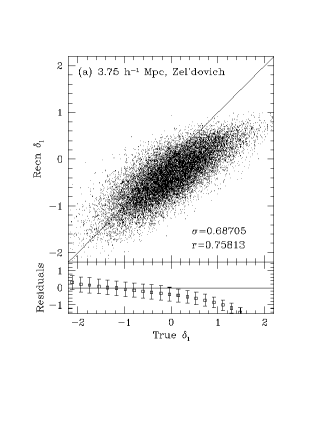
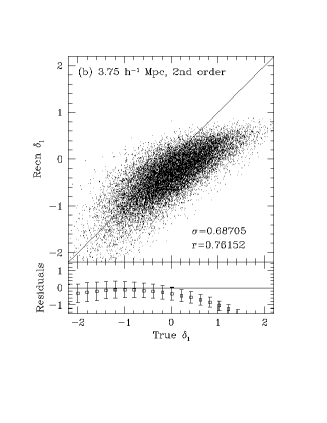
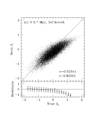
Figure 3: Reconstruction of initial conditions with XTRACE. Upper panels with 3.75 $h^{-1}\;{\rm Mpc}$ smoothing; lower panels with 5 $h^{-1}\;{\rm Mpc}$ smoothing. Panels on the left show the Zel’dovich approximation and panels on the right show 2nd order Lagrangian perturbation theory.

To suppress errors arising from the highly non-linear dynamics inside relaxed structures, we have collapsed the “fingers of God” in redshift-space. Following Gramann, Cen & Gott (1994), groups have been found with a friends-of-friends algorithm, with radial and tangential linking lengths respectively of 3 and 0.5 $h^{-1}\;{\rm Mpc}$. The radial component of the distance of each galaxy from the centroid of the group is rescaled so that the groups become spherical on average. This procedure was applied to typically 50 or so prominent groups and clusters in the simulated galaxy catalogues. In this way, the high peaks of the redshift-space density are slightly more enhanced. On the scales tested, the collapse of the fingers of God produces a slight improvement of the results.

5.2 Smoothing strategies

As already discussed in Section 4, smoothing is necessary to derive a continuous density field from the simulated catalogues and to suppress highly non-linear structures. When we use the full evolved density field from a simulation as an input to the reconstruction algorithms, a moderate smoothing in Eulerian space is performed. As described in Section 4, adaptive smoothing is too slow to be applied to $\ga 100,000$ point masses.

The simulated galaxy catalogues are smoothed with the adaptive smoothing algorithm described in Section 4. The reference smoothing radius is held fixed within a characteristic distance of either $R_{*}=50$ or $80$ $h^{-1}\;{\rm Mpc}$, so that at this distance 10 galaxies are on average contained in the filter volume (defined as $V_{G}=(2\pi)^{1.5}R_{sm}^{3}$, where $R_{sm}$ is the smoothing radius). At larger radii, the smoothing radius is increased to compensate for the selection function, so that there are 10 galaxies on average inside the filter volume. The reference smoothing radii are 5.15 or 7.65 $h^{-1}\;{\rm Mpc}$, when the characteristic distance $R_{*}$ is 50 or 80 $h^{-1}\;{\rm Mpc}$. The density field within $R_{*}$ is well sampled and is reconstructed with a constant reference smoothing radius, while the outer parts are used just to give the external tides to the inner parts of the simulated catalgues. The fact that the density field is smoother in the outer parts is an advantage for the reconstruction method, as it reduces the sensitivity to the boundary conditions (see Section 2.2).

It is worth noting that the smoothing requires knowledge of the selection function to determine the density contrast. The same selection function is applied to the N-body simulations to select the galaxies in real space and to estimate the density contrast in redshift space. This is not strictly correct, as the selection functions in real and redshift space will be slightly different. However, as pointed out by Hamilton (1998), these differences will be small for an all-sky catalogue. We have checked that the differences between the real-space and redshift-space selection functions for our simulated catalogues are indeed negligible.

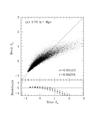
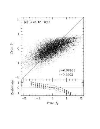
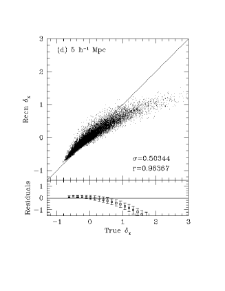
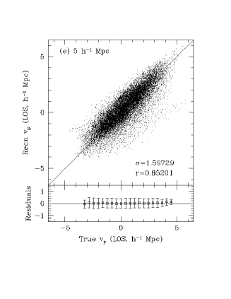
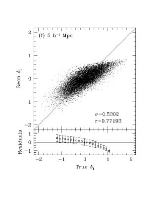
Figure 4: Reconstruction with ZTRACE with smoothing of 3.75 $h^{-1}\;{\rm Mpc}$ (upper panels) and 5 $h^{-1}\;{\rm Mpc}$ (lower panels).

5.3 Results with XTRACE

The complete real-space density field from the EdS simulation has been given as an input to XTRACE. This allows us to compare our results with those of Narayanan & Croft (1998). The input real space density field is smoothed with Gaussian filters of widths 3.75 $h^{-1}\;{\rm Mpc}$ and 5 $h^{-1}\;{\rm Mpc}$. Fig. 3 shows the scatterplots of true and reconstructed linear density fields. In these comparisons, the true linear density field has been smoothed with the same Gaussian filters. The reconstruction algorithm introduces some noise at the level of the grid cell, which is difficult to subtract without removing true power present at small scales. To suppress this noise, a Gaussian smoothing of 2.5 $h^{-1}\;{\rm Mpc}$ has been applied to the reconstructed fields. Finally, both the Zel’dovich and the 2nd order reconstructions are shown.

The following points can be noted from Fig. 3:

1. The reconstructed linear density rarely exceeds the value of unity. This is a true physical effect as the high peaks in the evolved density fields are in the multi-stream regime but are assumed to be in the the mildly non-linear phase in the reconstruction. As a consequence, they are reconstructed as though they evolved from shallower peaks with linear density $\la 1$. (In fact, in a general pancake-like collapse, the real space density contrast is $\delta_{r}\approx 4$ when the extrapolated linear density contrast is $\delta_{l}\simeq 0.8$.)

2. With larger smoothing, the reconstructed linear density field is less noisy, with no additional bias. This is due to the noise introduced at small scales by highly non-linear dynamics. Some smoothing is required to suppress this noise.

3. The 2nd order dynamics tends to improve the correlation with the true field slightly, but induces some further bias in recovering underdensities; as discussed in Section 2, this is because 2nd order perturbation theory is inaccurate for deep underdensities. As a consequence, going to 2nd order does not improve the reconstruction scheme significantly.

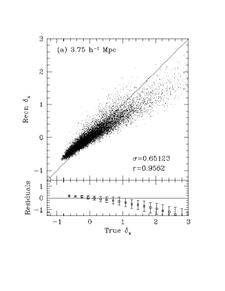
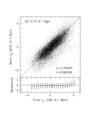
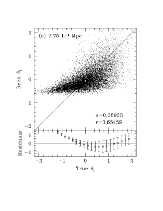
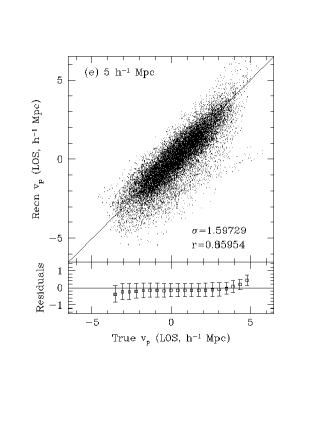
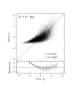
Figure 5: Reconstruction with LTRACE, with smoothing of 3.75 $h^{-1}\;{\rm Mpc}$ (upper panels) and 5 $h^{-1}\;{\rm Mpc}$ (lower panels).

The comparison with the results of Narayanan & Croft (1998) are not completely straightforward, as they use simulations with a smaller box (200 $h^{-1}\;{\rm Mpc}$) normalized to have $\sigma_{8}=1$. Nonetheless, it appears that the performance of XTRACE is comparable or even better than other Zel’dovich-based approximations, especially for underdensities. The XTRACE algorithm performs similarly to the hybrid Gaussianization model of Narayanan & Weinberg (1998), in which the PDF of initial conditions is forced to be Gaussian. The PIZA method of Croft & Gatzañaga (1997) appears to perform better than both XTRACE and the Narayanan & Weinberg algorithm, recovering linear density contrasts greater than unity, though underdensities are recovered with a slightly biased. The smaller scatter in the PIZA reconstruction arises because the method uses the final positions of the N-body particles and hence there is no need to smooth the evolved density field in Eulerian space. It would be interesting to investigate the performance of PIZA on simulated galaxy redshift surveys which include a realistic selection function.

5.4 Results with ZTRACE

As a first step, the full redshift-space density field of the evolved simulation is given as input to ZTRACE and LTRACE. The density field is suppressed, as described in Section 2.2, at radii greater than 84 $h^{-1}\;{\rm Mpc}$ from the origin. As in the test of XTRACE, we smooth the input redshift-space density field with Gaussian filters of widths 3.75 $h^{-1}\;{\rm Mpc}$ and 5 $h^{-1}\;{\rm Mpc}$ and smooth the output density and velocity fields on a scale of 2.5 $h^{-1}\;{\rm Mpc}$ to suppress the noise introduced by the reconstruction algorithm. The true fields from the simulations are smoothed with the same filters as the input redshift-space density field. The comparisons are shown in Figure 4 for radii less than 84 $h^{-1}\;{\rm Mpc}$ and larger than 10 $h^{-1}\;{\rm Mpc}$ (excluding the central region, which is not recovered accurately as described in Section 2.2). Note that no attempt has been made in these comparisons to collapse “fingers of God” in the input redshift-space density field. Fig.4 shows the results from ZTRACE for the real-space density field, the peculiar velocity and the linear density. Fig. 5 shows the same results obtained with LTRACE.

The following points can be noted from Figs. 4 and 5:

1. Smoothing on a larger scale decreases the scatter in the Figures without introducing a larger bias.

2. The highest peaks in the real-space density are not correctly recovered. As in the application of XTRACE, this is because smoothing in Eulerian space introduces bias and because the reconstruction algorithm does not correctly model multi-stream regions.

3. The peculiar velocity is recovered in an almost unbiased way.

4. The reconstruction of the linear density field is noisy; again, the density peaks with $\delta_{l}>1$ are considerably suppressed. Underdensities are recovered in a biased way due to the smoothing in Eulerian space.

5. ZTRACE always performs better than LTRACE; however, both the real-space density field and the LOS peculiar velocities are reconstructed fairly well by linear theory. The linear density field recovered by LTRACE is, however, very different from the true one.

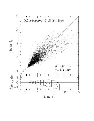
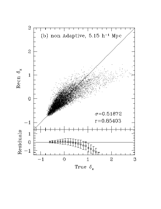
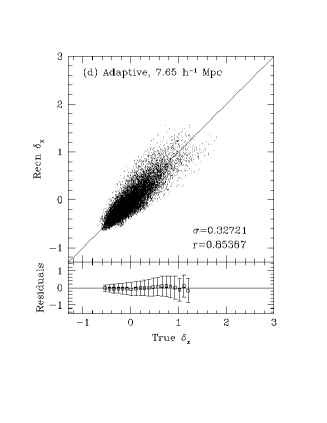
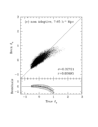
Figure 6: Reconstruction of the real-space density field with ZTRACE and LTRACE within 50 $h^{-1}\;{\rm Mpc}$ (upper panels, smoothing of 5.15 $h^{-1}\;{\rm Mpc}$) and 80 $h^{-1}\;{\rm Mpc}$ (lower panels, smoothing of 7.65 $h^{-1}\;{\rm Mpc}$).

This analysis shows that the ZTRACE procedure improves over linear theory, especially in recovering the initial density field. We will show below that the use of adaptive smoothing in ZTRACE gives a further improvement making it a useful tool for the analysis of real galaxy redshift surveys.

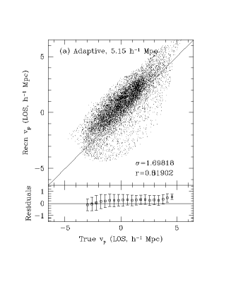
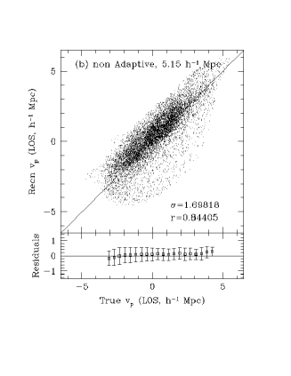
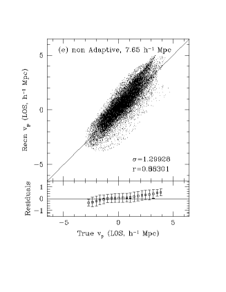
Figure 7: Reconstruction of the LOS peculiar velocity (expressed as an apparent displacement) with ZTRACE and LTRACE, within 50 $h^{-1}\;{\rm Mpc}$ (upper panels, smoothing of 5.15 $h^{-1}\;{\rm Mpc}$) and 80 $h^{-1}\;{\rm Mpc}$ (lower panels, smoothing of 7.65 $h^{-1}\;{\rm Mpc}$).

Figs. 6 to 8 show the performance of ZTRACE and LTRACE in reconstructing the real-space density, LOS velocity and initial density, from the simulated PSCz catalogue described in Section 5.1. We provide the redshift-space density field as input smoothed with adaptive and non-adaptive Gaussian filters as described in Section 5.2. The figures show results for the ZTRACE algorithm for smoothing radii of 5.15 and 7.65 $h^{-1}\;{\rm Mpc}$ (for adaptive smoothing these numbers refer to the values of the reference radii). The upper panels show the reconstruction within 50 $h^{-1}\;{\rm Mpc}$ of the origin and the lower panels show results within 80 $h^{-1}\;{\rm Mpc}$. To suppress the grid-level noise introduced by the reconstruction, the recovered fields are smoothed on a scale of 2.5 $h^{-1}\;{\rm Mpc}$ in the 50 $h^{-1}\;{\rm Mpc}$ case, and on a scale of 3.75 $h^{-1}\;{\rm Mpc}$ in the 80 $h^{-1}\;{\rm Mpc}$ case. The results for the LTRACE algorithm with non-adaptive smoothing are also shown in the figures.

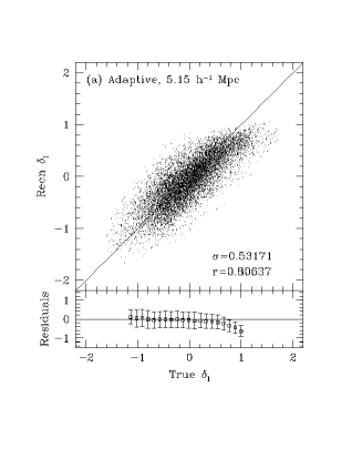
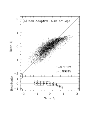
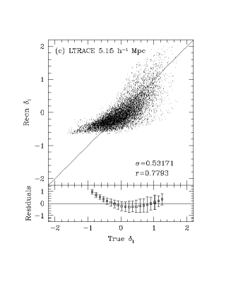
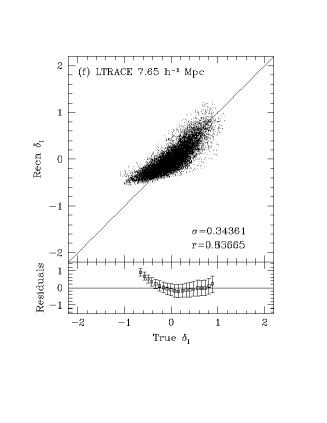
Figure 8: Reconstruction of the linear density with ZTRACE and LTRACE, within 50 $h^{-1}\;{\rm Mpc}$ (upper panels, smoothing of 5.15 $h^{-1}\;{\rm Mpc}$) and 80 $h^{-1}\;{\rm Mpc}$ (lower panels, smoothing of 7.65 $h^{-1}\;{\rm Mpc}$).

For reference, Fig. 9 shows a comparison between the redshift-space density field, as estimated from the simulated PSCz catalogue, and the true redshift-space density of the full simulation smoothed with constant smoothing radii of 5.15 and 7.65 $h^{-1}\;{\rm Mpc}$. The dominant source of noise in this figure arises from the estimation of the density field from the sparsely sampled redshift catalogue as we have discussed in Section 4. The bias at high densities seen when adaptive smoothing is applied to the redshift catalogue is an artifact of comparing the adaptively smoothed field with the non-adaptively smoothed density estimates from the N-body simulation.

Fig. 10 shows the reconstructed initial densities from ZTRACE and LTRACE with 7.65 $h^{-1}\;{\rm Mpc}$ smoothing, compared with the true initial density field of the simulation along a slice of the computational volume centred on the observer. The ZTRACE algorithm gives a good representation of the initial conditions even at the edge of the simulated redshift survey. In contrast, the initial conditions recovered by LTRACE resemble a heavily smoothed (and biased) version of the initial conditions. Fig. 8 provides a more quantitative comparison of the initial densities recovered by these algorithms.

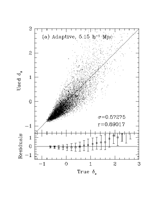
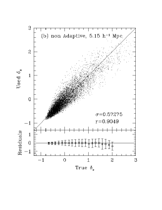
Figure 9: Reconstruction with ZTRACE, within 50 $h^{-1}\;{\rm Mpc}$ (upper panels, smoothing of 5.15 $h^{-1}\;{\rm Mpc}$) or 80 $h^{-1}\;{\rm Mpc}$ (lower panels, smoothing 7.65 $h^{-1}\;{\rm Mpc}$). Redshift-space densities used as an input to the ZTRACE algorithm compared with the smoothed true density from the full output of the simulation. (a) and (c) shows adaptive smoothing with a reference radii of 5.15 $h^{-1}\;{\rm Mpc}$ and 7.65 $h^{-1}\;{\rm Mpc}$; (b) and (d) show non-adaptive smoothing with radii of 5.15 $h^{-1}\;{\rm Mpc}$ and 7.65 $h^{-1}\;{\rm Mpc}$.

From this analysis we conclude the following:

1. From Fig. 9, we see that the scatter in the density estimate is large, as expected from the analysis of Section 4. Adaptive smoothing increases the noise slightly.

2. Adaptive smoothing leads to an accurate reconstruction of the real-space density field (Fig. 6). Even high-density peaks with $\delta\sim 1$ are recovered with little bias. In contrast, the real space densities recovered with non-adaptive smoothing are strongly biased at density contrasts approaching unity.

3. All of the methods recover the LOS peculiar velocities to comparable accuracy (Fig. 7). The peculiar velocity field is more strongly correlated than the density field and the number of effectively independent volumes in our $50$ and $80$ $h^{-1}\;{\rm Mpc}$ spheres is relatively small. The velocity fields thus show structure arising from distinct objects (especially in the lower panels of Fig. 7).

4. Adaptive smoothing significantly improves the accuracy of the linear density field reconstruction from ZTRACE algorithm (Figs. 8 and 10). The recovered linear density field is almost unbiased, even to density contrasts approaching unity. Furthermore, the adaptive ZTRACE linear density field has the correct variance.

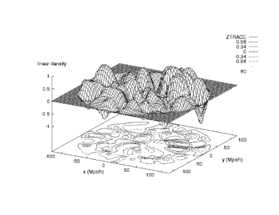
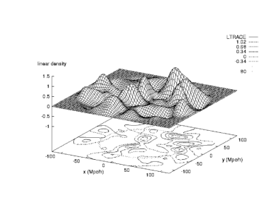
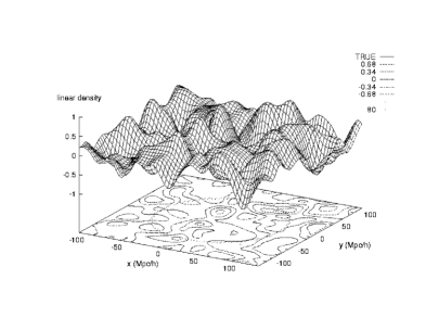
Figure 10: Reconstruction of the linear density from a simulated PSCz redshift survey along a thin slice centered on the observer. The upper two figures show the results from ZTRACE and LTRACE, within 80 $h^{-1}\;{\rm Mpc}$ (smoothing of 7.65 $h^{-1}\;{\rm Mpc}$), compared to the true linear density field plotted at the bottom. The contours show one, two and three $\sigma$ levels and the radius of 80 $h^{-1}\;{\rm Mpc}$ is shown by the dotted lines.

5.5 The PDF of the Reconstructed Linear Density

One of the problems with many of the reconstruction methods described in the Introduction is that they are not able to reproduce the correct PDF of the initial conditions. This problem can be avoided heuristically by “Gaussianizing” the reconstructed field as described by Weinberg (1992) and Narayanan and Weinberg (1998). Clearly, it is important to develop techniques for recovering the initial conditions without making any specific assumptions concerning the PDF. Fig. 11 shows the 1-point PDF of the reconstructed linear density computed from ZTRACE compared to the Gaussian PDF of the true initial conditions. The adaptive ZTRACE algorithm reproduces the true PDF very accurately, except for the tail at $\delta_{l}>1$ which is severely truncated. The PDF of underdense regions, even the tail at large negative amplitudes, is reproduced extremely well by the adaptive ZTRACE algorithm.

When applied to real redshift surveys, this could provide an interesting test of the Gaussianity of the initial conditions. More realistically, the PDF of the initial conditions recovered by ZTRACE could be useful in constraining models of bias.

Figure 11: PDF of the linear density recovered by ZTRACE with adaptive and non-adaptive smoothing compared to the true Gaussian PDF of the N-body simulation. The dotted lines show the PDF’s recovered by LTRACE. Panel (a) shows the PDF’s within 50 $h^{-1}\;{\rm Mpc}$and a smoothing of 5.15 $h^{-1}\;{\rm Mpc}$; panel (b) shows the PDF’s within 80 $h^{-1}\;{\rm Mpc}$and a smoothing of 7.65 $h^{-1}\;{\rm Mpc}$.

5.6 Dependence on Cosmology

The reconstruction in the case of an open universe is carried out in exactly the same way as in the EdS universe. The dependence on cosmology enters the formalism only through the $f(\Omega)$ function (Eq. 2.1), which determines the strength of the peculiar velocities, and through the growing mode $D(t)$ (Eqs. 2, 3 and 4), which determines the rescaling of the initial density to the present time (the linear density $\delta_{l}$). As expected, the results obtained in the open case are indistinguishable from those presented for the EdS model in the previous sections.

It is interesting to apply the ZTRACE reconstruction to the evolved density field in an open universe but assuming an EdS cosmology. In this way we can test the error made by ZTRACE as a result of assuming the wrong cosmology. In this test the initial density field is rescaled to the present time with the correct growing mode. Fig. 12 shows the recovery of the real-space density, LOS peculiar velocity and linear density when ZTRACE is applied to a simulated PSCz catalogue within 80 $h^{-1}\;{\rm Mpc}$ (with adaptive smoothing). As expected, the LOS peculiar velocity is recovered up to a factor $\Omega^{0.6}\simeq 0.48$ (Fig. 11b), which means that the inferred LOS displacements are overestimated by nearly a factor 2; in practice this number is degenerate with the linear bias parameter $b$ (which is unity in the simulations). This overestimate of the peculiar velocities should lead to an underestimate of overdensities and an overestimate of underdensities in both the real-space and the linear density fields. These effects are indeed present in Figs. 12a and c, but are almost imperceptible. This is not surprising because the bias cannot be larger than the differences between the real-space and redshift-space densities, which are small compared to the scatter in the reconstruction.

This is another illustration of the intrinsic limits of reconstruction algorithms applied to realistic galaxy surveys. As a consequence, while the correct, unbiased, reconstruction of peculiar velocities requires correct knowledge of the underlying cosmological model, both the inferred real-space and the linear densities are robust with respect to cosmology. This has two consequences: (i) the recovery of initial conditions and of their PDF is insensitive to the assumed cosmology; (ii) the information on the cosmological model (actually the parameter combination $\Omega^{0.6}/b$) is contained almost exclusively in the peculiar velocities.

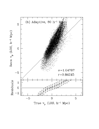
Figure 12: ZTRACE reconstruction using a PSCz catalogue generated from the open N-body simulation, but where we have assumed an EdS cosmology. The figures show results within 80 $h^{-1}\;{\rm Mpc}$ using an adaptive smoothing reference radius of 7.65 $h^{-1}\;{\rm Mpc}$.

6 Conclusions

We have described a reconstruction algorithm, ZTRACE, based on a self-consistent solution of the Zel’dovich dynamics of large-scale structure. Given an input (observable) density field in redshift space, this algorithm reconstructs the real-space density field, the LOS peculiar velocities and the initial conditions which evolve into this redshift-space density field according to the Zel’dovich approximation. The method can be easily extended to second order in Lagrangian perturbation theory, though we have demonstrated using N-body simulations that this extension does not give any significant improvement in the reconstruction.

The ZTRACE algorithm has been tested by recovering the initial conditions of N-body simulations of CDM dominated EdS and open universes with scale-invariant initial power spectra. The redshift-space density was estimated using all of the particles in the simulation and from simulated galaxy catalogues with the selection function of the IRAS PSCz survey under the assumption that galaxies trace mass. We have also constructed a test version of the algorithm (XTRACE), which requires the evolved real-space density field as input, and a linear-theory version (LTRACE).

The major source of noise and bias in the reconstructions comes from the density field estimates. For simulated PSCz catalogues with smoothings of several $h^{-1}\;{\rm Mpc}$, the dispersion in the density field estimates is comparable to the dispersion in the density field itself. The most significant problem revealed by our tests arose from the fact that smoothing in Eulerian space does not commute with the dynamics; it mixes the larger Lagrangian scales involved in overdensities with the smaller ones involved in underdensities. The problem can be solved, at the expense of increased noise in the density estimates, by applying a mass-preserving adaptive smoothing to the density field.

As a consequence of noise in the density field estimates, the ability of ZTRACE to recover the real-space density and the LOS peculiar velocities is not dramatically better than applying a simple algorithm based on linear theory. However, the use of adaptive smoothing allows ZTRACE to reconstruct the initial density field in an unbiased although noisy way, provided that the linearly extrapolated density does not exceed a value of unity. Higher extrapolated densities cannot be recovered accurately because of the presence of multi-stream and triple-valued regions, which violate the single-stream assumption of the Zel’dovich approximation. The PDF of the initial conditions is correctly reproduced by the reconstruction with ZTRACE to high accuracy, except for the tail of high overdensities at $\delta_{l}>1$.

We have shown that the Gaussian PDF of the initial conditions used in the N-body simulations is recovered from the input catalogues in which galaxies are assumed to trace the mass. If the relationship between the galaxy and the mass density is more complicated, as proposed, for example, by Mo & White (1996), Catelan et al. (1998) or Dekel & Lahav (1998), then the PDF of the initial conditions recovered by assuming that galaxies trace the mass may be non-Gaussian. In a future paper, the ZTRACE method will be applied to the reconstruction of the initial conditions of our local Universe from the IRAS PSCz catalogue and we will investigate how the reconstructed PDF can be used to constrain models of non-linear bias.

References

- [1] Baker J. E., Davis M., Strauss M. A., Lahav O., Santiago B., 1998, ApJ, submitted (astro-ph/9802173)
- [2] Bernardeau F., Kofman L., 1995, ApJ, 443, 479
- [3] Branchini E., Carlberg R. G., 1994, ApJ, 434, 37
- [4] Branchini E., Frenk C. S., Teodoro L., Schmoldt I., Efstathiou G., Saunders W., White S. D. M., Rowan-Robinson M., Sutherland W., Tadros H., Maddox S., Oliver S., Keeble O., 1998, in Evolution of Large Scale Structure – Garching 1998, in preparation
- [5] Branchini E., Plionis M., 1996, ApJ, 460, 569
- [6] Bouchet F.R., Colombi S., Hivon E., Juszkiewicz R., 1995, A&A, 296, 575
- [7] Buchert T., 1989, A&A, 223, 9
- [8] Buchert T., Ehlers J., 1993, MNRAS, 264, 375
- [9] Canavezes A., Springel V., Oliver S. J., Rowan-Robinson M., Keeble O., White S. D. M., Saunders W., Efstathiou G., Frenk C. S., McMahon R. G., Maddox S., Sutherland W., Tadros H., 1998, MNRAS, submitted (astro-ph/9712228)
- [10] Catelan P., 1995, MNRAS, 276, 115
- [11] Catelan P., Lucchin F., Matarrese S., Porciani C., 1998, MNRAS, 297, 692
- [12] Chodorowski M. J., Lokas E. L., Pollo A., Nusser A., 1998, MNRAS, 300, 1027
- [13] Couchman H., Thomas P., Pearce F., 1995, ApJ 452 797
- [14] Croft R. A. C., Gaztañaga E., 1997, MNRAS, 285, 793
- [15] Dekel A., Lahav O., 1998, ApJ, in press (astro-ph/9806193)
- [16] Efstathiou G. Bond J. R., White S. D. M., 1992, MNRAS, 258, 1P
- [17] Fisher K. B., Lahav O., Hoffman Y., Lynden-Bell D., Zaroubi S., 1995, MNRAS, 272, 885
- [18] Giavalisco M., Mancinelli B., Mancinelli P. J., Yahil A., 1993, ApJ, 411, 9
- [19] Gramann M., 1993a, ApJ, 405, 449
- [20] Gramann M., 1993b, ApJ, 405, L47
- [21] Gramann M., Cen R., Gott J. R., 1994, ApJ, 425, 382
- [22] Hamilton, A. J. S., 1998, D. Hamilton. ed., Ringberg Workshop on Large-Scale Structure. Kluwer Academic, Dortrecht
- [23] Hivon E, Bouchet F. R., Colombi S., Juszkiewicz R., 1995, A&A, 298, 643
- [24] Hudson M., 1994, MNRAS, 266, 475
- [25] Kaiser N., Efstathiou G., Ellis R., Frenk C., Lawrence A., Rowan-Robinson M., Saunders W., 1991, MNRAS, 252, 1
- [26] Kolatt T., Dekel A., Ganon G., Willick J. A., 1996, ApJ, 458 419
- [27] Lahav O., Lilje P. B., Primack J. R., Rees M. J., 1991, MNRAS, 251, 128
- [28] Linde A., 1990, Particle Physics and Inflationary Cosmology. Harwood Academic Publishers
- [29] Mo H. J., White S. D. M., 1996, MNRAS, 282, 347
- [30] Monaco P., 1997, MNRAS, 287, 753
- [31] Moutarde F., Alimi J.M., Bouchet F.R., Pellat R., Ramani A., 1991, ApJ, 382, 377
- [32] Narayanan V. K., Croft R. A. C., 1998, ApJ, submitted (astro-ph/9806255)
- [33] Narayanan V. K., Weinberg D., 1998, ApJ, submitted (astro-ph/9806238)
- [34] Nusser A., Dekel A., 1992, ApJ, 391, 443
- [35] Nusser A., Dekel A., Yahil A., 1995, ApJ, 449 439
- [36] Nusser A., Davis M., 1994, ApJ, 421, L1
- [37] Peebles P. J. E., 1980, The Large Scale Structure of the Universe. Princeton Univ. Press
- [38] Peebles P. J. E., 1989, ApJ, 344, L53
- [39] Peebles P. J. E., 1990, ApJ, 362, 1
- [40] Sahni V., Shandarin S.F., 1996. MNRAS, 282, 641
- [41] Saunders W., Sutherland W., Efstathiou G., Tadros H., Maddox S., McMahon R., White S., Oliver S., Keeble O., Rowan-Robinson M., Frenck C., 1994, in Maddox S. J., Aragon-Salamanca A., eds., Wide field Spectroscopy and the Distant Universe. World Scientific, Singapore, p. 88
- [42] Shaya E. J., Peebles P. J. E., Tully R. B., 1995, ApJ, 454, 15
- [43] Springel V., White S. D. M., Colberg J. M., Couchman H. M. P., Efstathiou G. p., Frenk C. S., Jenkins A. R., Pearce F. R., Nelson A. H., Peacock J. A., Thomas P. A., 1998, MNRAS, submitted (astro-ph/9710368)
- [44] Susperregi M., Buchert T., 1997, A&A, 323, 295
- [45] Sutherland W., Tadros H., Efstathiou G., Frenk C. S., Keeble. O., Maddox S., McMahon R. G., Oliver S., Rowan-Robinson M., Saunders W., White S. D. M., 1999, MNRAS, in press (astro-ph/9901189)
- [46] Taylor A. N., Rowan-Robinson M., 1993, MNRAS, 265, 809
- [47] Webster M., Lahav O., Fisher K., 1997, MNRAS, 287, 425
- [48] Weinberg D. H., 1992, MNRAS, 254, 315
- [49] Yahil A., Strauss M. A., Davis M., Hucra J. P., 1991, ApJ, 372, 380
- [50] Zel’dovich, Ya.B. 1970, Astrofizika 6, 319 (transl.: 1973, Astrophysics 6, 164)