An extinction study of the Taurus Dark Cloud Complex

Abstract

We present a study of the detailed distribution of extinction in a region of the Taurus dark cloud complex. Our study uses new $BVR$ images of the region, spectral classification data for 95 stars, and IRAS Sky Survey Atlas (ISSA) 60 and 100 µm images. We study the extinction of the region in four different ways, and we present the first inter-comparison of all these methods, which are: 1) using the color excess of background stars for which spectral types are known; 2) using the ISSA 60 and 100 µm images; 3) using star counts; and 4) using an optical ($V$ and $R$) version of the average color excess method used by Lada et al. (1994). We find that all four methods give generally similar results–with important exceptions. As expected, all the methods show an increase in extinction due to dense dusty regions (i.e. dark clouds and IRAS cores), and a general increase in extinction with increasing declination, due to a larger content of dust in the northern regions of the Taurus dark cloud complex. Some of the discrepancies between the methods are caused by assuming a constant dust temperature for each line of sight in the ISSA extinction maps and not correcting for unexpected changes in the background stellar population (i.e. the presence of a cluster or Galactic gradients in the stellar density and average V R color). To study the structure in the dust distribution, we compare the ISSA extinction and the extinction measured for individual stars. From the comparison, we conclude that in the relatively low extinction regions studied, with $0.9<A_{V}<3.0$ mag (away from filamentary dark clouds and IRAS cores), there are no fluctuations in the dust column density greater than 45% (at the 99.7% confidence level), on scales smaller than 0.2 pc. We also report the discovery of a previously unknown open cluster of stars behind the Taurus dark cloud near R.A 4h19m, Dec. 27°30′ (B1950).

Accepted by The Astrophysical Journal

1 Introduction

In order to understand how molecular clouds evolve and eventually produce stars, it is necessary to study the distribution of their star-forming matter. Since the clouds’ main constituent, molecular hydrogen, is generally unobservable, it is necessary to use other tracers, whose abundance relative to hydrogen can be reliably estimated, to map out the distribution of material. The extinction of background starlight is the result of the absorption and scattering of photons off dust grains; so, for a given line of sight, the amount of extinction is directly proportional to the amount of dust. If the gas-to-dust ratio is known and constant (e.g. Bohlin et al. 1978), then a detailed study of the dust distribution in a cloud serves as a detailed study of its mass distribution.

The study of fluctuations in the dust distribution is also interesting independent of its usefulness as a mass tracer. Strong fluctuations in the dust distribution have considerable impact on both the physics and chemistry of the interstellar medium (ISM), which both depend heavily on the extinction (opacity) structure on all scales (see Thoraval et al. 1997, and references therein). In addition, knowledge of the spatial structure and amount of extinction in the Galactic ISM is important as it effects the apparent colors of background sources, such as stars and galaxies.

The most direct measure of reddening is the color excess of a star with known spectral type. Unfortunately, mapping out extended distributions of extinction (reddening) by obtaining photometry and a spectrum for large numbers of stars is very tedious and time consuming, and usually impractical. Therefore, the traditional way of undertaking an extinction study of a fairly large region of the sky has been, until recently, through the use of optical star counts using photographic plates (Bok & Cordwell 1973). This method can only be used up to an extinction of approximately 4 mag, with a resolution of $\sim$2.5′. Thankfully, recent advances in technology have led to the development of new methods of deriving the extinction in dark cloud regions. For example, in a study of the structure of nearby dark clouds, Wood et al. (1994) use 60 and 100 µm images taken by IRAS to calculate 100 µm optical depth, from which they obtain the extinction ($A_{V}$). Lada et al. (1994; hereafter LLCB) took advantage of the improvements in infrared array cameras to devise a clever new method of measuring extinction. The LLCB technique, which combines measurements of near-infrared ($H$ and $K$) color excess and certain techniques of star counting, has a higher angular resolution and can probe greater optical depths than that achieved by optical star counting alone.

In this study we use four different methods of measuring $A_{V}$, utilizing: 1) the color excess of individual background stars for which we could obtain spectral types; 2) ISSA 60 and 100 µm images to estimate dust opacity; 3) traditional star counting; and 4) an optical ($V$ and $R$) version of the average color excess method used by Lada et al. (1994). To our knowledge, this is the first time that all of these different methods have been directly intercompared. We describe the acquisition and reduction of the data in Section 2. In Section 3 we present the results of the observations, and in Section 4 we offer analysis and discussion. Readers interested primarily in intercomparison of the various methods and limits on density fluctuations should skim sections 2 and 3 and focus more on Section 4 and 5. In Section 5 we compare and rate the four different methods of obtaining $A_{V}$. We devote Section 6 to our conclusions.

2 Data

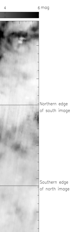
Figure 1: Extinction ($A_{V}$) map of part of the Taurus dark cloud region. The map was obtained using the method described in §2.3. The two cuts for which we have photometric (CCD) data are shown. The two filamentary dark clouds L1506 and B216-217 and the three IRAS cores Tau M1, Tau B5 and Tau B11 are identified. The star symbols represent the position of the stars that were classified by spectra. The horizontal lines mark the northern and southern edges of the two images that were used to make this map.

The new photometric and spectroscopic observations used in this paper were originally obtained to conduct the polarization-extinction study described in Arce et al. (1998). The photometry consists of $B$, $V$ and $R$ CCD images of two 10 arcmin by $\sim$ 5 deg “cuts” through the Taurus dark cloud complex (see Figure 1). In the spectroscopic observations, we observed 95 stars (most of them in cut 1), in order to determine their spectral types. The cuts shown in Figure 1 pass through two well known filamentary dark clouds (L1506 and B216-217, both at a distance of 140 pc from the Sun) as well as very low extinction regions, giving our photometric observations a fairly large dynamic range in extinction. In the spectroscopic observations, we selected our target stars along the two cuts by virtue of their relative brightness, in that we attempted to exclude foreground stars by not selecting stars which appear unusually bright. Table 1 lists the spectral type, apparent $V$ magnitude and $B-V$ color, and the derived spectroscopic parallax distance for each target star. Our stellar sample has only one star with a distance less than 140 pc, which confirms that we largely succeeded in excluding foreground stars. In addition to the new photometric and spectroscopic observations we also obtained co-added images of flux density from the IRAS Sky Survey Atlas (ISSA), in order to examine the far-infrared emission from dust in the region.

2.1 Photometric Data

The broad band imaging data of the two cuts (Figure 1) through the Taurus dark cloud complex were obtained using the Smithsonian Astrophysical Observatory (SAO) AndyCam on the Fred Lawrence Whipple Observatory (FLWO) 1.2-meter telescope on Mt. Hopkins, Arizona. AndyCam is a camera with a thinned back-side illuminated AR coated Loral $2048\times 2048$ CCD chip. All the frames were taken in $2\times 2$ bin mode, giving a plate scale of 0.63 arcsec per pixel. In 1995 November, a total of 64 frames in different positions in the sky were taken in the $B$, $V$ and $R$ bands, where $R$ is the Cousins $R$ band filter with an effective wavelength equal to 0.64 µm. In each position we obtained one 200 second exposure for each broad-band filter. Each telescope pointing was a little less than 10′ north of the previous position, and since each frame is slightly larger than 10′ $\times$ 10′, there is a small sky overlap between the frames successive positions. The first cut extends from declination of 22°30′ to 28°20′, centered on right ascension 4h 22m 36s (J2000), with a total of 36 frames. The second cut extends from declination 24°00′ to 28°30′, centered on right ascension 4h 21m 29s (J2000), with a total of 28 frames. In addition to the frames acquired in November 1995, seventeen frames were taken in the $U$, $B$, and $V$ bands in October 1996, four frames were taken in the $B$ and $V$ bands in November 1996, and two frames were taken in the $B$ and $V$ bands in March 1997 —all with the same instrument configuration as the November 1995 frames. The additional frames were taken because: not all of the original frames were of good quality; several frames were of regions of special interest around the 2 dark clouds peripheries (outside the cuts) which the original frames did not include; and because shorter exposure images of some of the regions covered by the original frames were needed. The exposure times were 80, 150, and 200 sec for $V$, $B$, and $U$, respectively, for frames of new sky positions, and 30 sec in $V$, 50 sec in $B$, and 100 sec in $U$ for frames with repeated positions in the sky.

All of the stellar photometric data reduction was done using standard Image Reduction and Analysis Facility (IRAF) routines. For stars whose spectra had been measured (see §2.2), photometry was obtained in the flat-fielded, background-subtracted images using the APPHOT routine. After analyzing the dependence of magnitude value with aperture size in the standard stars for all nights, it was decided to use an aperture radius of 14 pixels. With this aperture size, less than 10% of the stars in the most crowded field, with $R$-band apparent magnitude ($m_{R}$) between 14.5 and 18.0 mag, have neighbors within the aperture. The correction to the standard photometric system was done using Landolt standards (Landolt 1992). A set of standards were observed for each night, at different times of the night, at varying airmasses. These were then used to solve a set of linear equations that would give the stars’ $V$ magnitude, B V and V R colors using the routines in the IRAF package PHOTCAL. The errors obtained from the APPHOT routine, and the errors in the transformation equation fit were summed in quadrature to give the final errors in the photometry. These were $\pm 0.02$ to 0.06 mag for $V$ and B V for stars with $V$ between 12.3 and 17.4 mag. We calculated the photometry of the standard stars used to derive the transformation equation and compared our results with those quoted by Landolt (1992). By doing so we convinced ourselves that the value of our final 1 $\sigma$ errors (Table 1) are a reasonably good estimation of the true photometry uncertainties.

In addition to obtaining apparent magnitudes and colors for stars, the photometric data were also used to do a star count of the region. The routine DAOFIND was used to detect sources in the $R$ filter frames. This routine automatically detects objects that are above a certain intensity threshold, and within a limit of sharpness and roundness, all of which the user specifies. We used a finding threshold of 5 times the rms sky noise in each frame. The objects detected by the routine are then stored in a file with the objects’ coordinates. Although care was taken to select a limit of sharpness and roundness so that DAOFIND would only detect stars, other objects (like cosmic rays and galaxies) were also detected, and some stars clearly above the threshold level were not detected. Thus, the $R$ frames were painstakingly inspected visually to erase detected objects that were not stars, and add the few stars that were clearly above the threshold, but were not originally detected. We obtained the photometry of all the stars in the sample and then made a histogram (Figure 2) of the number of stars versus apparent $R$ magnitude in order to study the completeness of the sample. From Figure 2 we estimate the upper completeness limit to be $m_{R}\approx 18.0$ mag. Stars brighter than 14.5 mag in the $R$-band 200 second exposures are saturated, thus the photometry of stars with $m_{R}<14.5$ is unreliable. Therefore we estimate that our sample is 90% (or more) complete for stars with $14.5\leq m_{R}<18.0$.

2.2 Spectroscopic Data

The spectra of 95 stars along the cuts were obtained using the SAO FAST spectrograph on the FLWO 1.5-meter telescope on Mt. Hopkins, Arizona. The observations were carried out during the Fall trimesters of 1995 and 1996. FAST was used with a 3″ slit and a 300 line mm^-1 grating. This resulted in a resolution of $\sim$ 6 Å, a spectral coverage of $\sim 3800$ Å (from approximately 3600 to around 7400 Å), a dispersion of 1.47 Å/pixel and 1.64 pixels/arcsec along the dispersion axis.

The spectrum of each star was used to derive its spectral type. In order to spectroscopically classify the stars, we followed O’Connell (1973) and Kenyon et al. (1994) and computed several absorption line indices from the spectra:

$$I_{\lambda}=-2.5~{}{\rm log}\left[\frac{F(\lambda_{2})}{F^{\prime}(\lambda_{2})}\right]$$ (1)

where

$$F^{\prime}(\lambda_{2})=F(\lambda_{1})+\left[F(\lambda_{3})-F(\lambda_{1})\right]\left[\frac{\lambda_{2}-\lambda_{1}}{\lambda_{3}-\lambda_{1}}\right]$$ (2)

is the interpolated continuum flux at the feature, $\lambda_{1}$ and $\lambda_{3}$ are continuum wavelengths, $\lambda_{2}$ is the feature wavelength, and $F(\lambda_{i})$ is the average flux in erg cm^-2 s^-1 Å^-1 over a bandwidth specified in Table II of O’Connell (1973). We measured the Ca II H ($\lambda 3933$), H$\delta$ ($\lambda 4101$), CH ($\lambda 4305$), H$\epsilon$ ($\lambda 4340$), H$\zeta$ ($\lambda 4861$), and Mg I ($\lambda 5175$) indices of our program stars and then compared them to the indices of main sequence stars in the Jacoby et al. (1984) atlas. The indices have errors of $5-10\%$ depending on the signal to noise of the spectrum. This method resulted in spectral classification of most of the stars observed with accuracy of $\sim\pm 1-2$ subclasses for spectral types A through F and $\pm 2-4$ subclasses for stars with spectral type G. Stars with spectral types earlier than A0 were not found, and stars later than G9 were not included in the sample due to the low accuracy in their spectral classification and reddening corrections. All the stars were assumed to be main sequence stars (luminosity type V). Kenyon et al. (1994) estimate, and also obtain, that $\sim$ 10% of their magnitude-limited sample of A–F stars in the Taurus region are giants. If we use this result with our magnitude-limited sample it would mean that only $\sim$7 stars of our 69 A–F stars are giants. In addition, the intrinsic B V color of main sequence A and F stars differs by less than 0.05 mag from the intrinsic B V of luminosity type III and type II stars. Of the G stars, no more than 5 out of a total of 26 should be giant stars (Mihalas & Binney 1981; Table 4-9). Hence we are not introducing large errors in the extinction of each star by assuming that all of the stars we classified are luminosity type V.

Once each star was classified, its reddening was calculated. Intrinsic B V values for each spectral type were obtained from Table A5 in Kenyon & Hartmann (1995). The observed B V value, from the photometric study, was then used to obtain the color excess: $E_{B-V}=(\bv)-(\bv)_{\circ}$, where (B V) is the observed color index and (B V)_∘ is the unreddened intrinsic color of the star. An error in the stellar classification of $\pm 1-2$ subclasses in A-F stars transforms into an error of $\pm 0.04-0.05$ mag in $E_{B-V}$, while an error in the stellar classification of $\pm 2-4$ subclasses in G stars transforms into an error of $\pm 0.05-0.08$ mag in $E_{B-V}$. We assumed that $A_{V}=R_{V}E_{B-V}$, with $R_{V}$ (the ratio of total-to-selective extinction) equal to 3.1 (Savage & Mathis 1979; Vrba & Rydgren 1985) —the validity of this assumption is discussed below. Using absolute magnitude values for each spectral type from Lang (1991), we then obtained distances for each star (see Table 1).

When we calculated the extinction to each star using a constant value of $R_{V}=3.1$, we made the implicit assumption that the ratio of total-to-selective extinction is constant for different lines of sight. In fact, $R_{V}$ varies along different lines of sight in the Galaxy and only has a mean of $\sim 3.1$ (Savage & Mathis 1979). In contrast with other regions, the Taurus-Auriga molecular cloud complex seems to have a fairly constant interstellar reddening law with $R_{V}\approx 3.1$ through most of the region (Vrba & Rydgren 1985; Kenyon et al. 1994). Our $BVR$ photometry is not ample enough to derive $R_{V}$ for each line of sight. We would need observations at shorter wavelengths to be able to independently obtain the value of the ratio of total-to-selective extinction for each line of sight we observed. Thus we decided to use the ISM (and Taurus) average of $R_{V}=3.1$, and to caution the reader that we do not take the errors caused by assuming a constant $R_{V}$ into account when we calculate the errors in $A_{V}$. In Section 3.1, we show how the ISSA data confirm that $R_{V}=3.1$ is a good estimate of the ratio of total-to-selective extinction for our region.

2.3 ISSA Data

The IRAS Sky Survey Atlas (ISSA) was used to obtain images of flux density at 60 and 100 µm of the Taurus dark cloud complex. Our region of interest lies in two different (but overlapping) ISSA fields. Each of these is a 500- by 500-pixel image, covering a 12.5° by 12.5° field of sky with a pixel size of 1.5′. The maps have units of MJy Sr^-1, are made with gnomic projection, have spatial resolution smoothed to the IRAS beam at 100 µm (approximately 5′), and the zodiacal emission has been removed from them. The 12.5° by 12.5° images were cropped in order to keep only the region of the Taurus dark cloud complex shown in Figure 1. This resulted in a total of four different images; two (60 and 100 µm) images of the northern part and two images of the southern part of the map.

Although they have the zodiacal emission removed, ISSA fields are not calibrated so that the “zero point” corresponds to no emission, so another “background” needs to be subtracted. This background subtraction procedure went as follows. First, the minimum value of each of the four 12.5° by 12.5° images (see Table 2) was obtained and subtracted from them. The resulting images were then used to obtain an optical extinction ($A_{V}$) map through a process to be discussed below. At this point, after just a simple subtraction of the minimum value in each image, the north and the south A_V maps (see Figure 1) did not agree within the errors in the region of overlap. So, the values used for the background subtraction were iterated until the best agreement for the overlap region was found, while keeping the background subtraction constants less than 1 MJy Sr^-1 away from the minimum flux value of the original 12.5° by 12.5° ISSA fields. Table 2 lists the values that were ultimately used for this purpose. These values resulted in a difference of 0.1 mag between the mean in the distribution of $A_{V}$ values in the northern image and the mean in the distribution of $A_{V}$ values in the southern image. Tests using other values for background subtraction showed that the resultant extinction values did not change significantly for small (less than $\sim$1 MJy Sr^-1) changes in the background subtraction constants. As discussed below, the offset between ISSA plates winds up being the limiting error in determining extinction from ISSA data.

The extinction map was computed from the ISSA images using a method very similar to that described by Wood, Myers & Daugherty (1994), and references therein. Note, however, that in their study, Wood et al. (1994) used IRAS images which had not gone through a zodiacal emission removal process. They devised their own zodiacal light subtraction, which they state is not very efficient for regions near the ecliptic, like Taurus. One of the regions they study was in fact the Taurus dark cloud region itself. We believe that our extinction map is of better quality due to the fact that we use ISSA images which have a more elaborate zodiacal light subtraction algorithm.

The 60 and 100 µm dust temperature, $T_{d}$, at each pixel in an image can be obtained by assuming that the dust in a single beam can be characterized by one temperature ($T_{d}$), and that the observed ratio of 60 to 100 µm emission is due to blackbody radiation from dust grains at $T_{d}$, modified by a power-law emissivity. The flux density of emission at a wavelength $\lambda_{i}$, is given by

$$F_{i}=\left[\frac{2hc}{\lambda^{3}_{i}}\frac{1}{e^{hc/\lambda_{i}kT_{d}}-1}\right]N_{d}\alpha\lambda_{i}^{-\beta}\Omega_{i}$$ (3)

where $N_{d}$ is the column density of dust grains, $\beta$ is the power-law index of the dust emissivity, $\Omega_{i}$ is the solid angle at $\lambda_{i}$, and $\alpha$ is a constant of proportionality.

In order to use equation 3 to calculate the dust color temperature ($T_{d}$) of each pixel in the image we have to make some assumptions. The first assumption is that the dust emission is optically thin. We believe this is a safe assumption because in our maps there is not a single line of sight that could be optically thick ($\tau_{100}>1$). In fact, the largest $\tau_{100}$ we find in our processed images is 0.002. The second assumption we have to make is that $\Omega_{60}\cong\Omega_{100}$, which is true for all ISSA images. With these two assumptions we can then write the ratio $R$ of the flux densities at 60 and 100 µm as:

$$R=\frac{F_{60}}{F_{100}}=0.6^{-(3+\beta)}\left[\frac{e^{144/T_{d}}-1}{e^{240/T_{d}}-1}\right]$$ (4)

In order to proceed we need to assume a value of $\beta$. For now we will assume that $\beta=1$, and we will discuss the implications of this assumption later on. We constructed a look-up table with the value of $R$ calculated for a wide range of $T_{d}$, with steps in $T_{d}$ of 0.05 K. For each pixel in the image, the table was searched for the value of $T_{d}$ that reproduces the observed 100 to 60 µm flux ratio. Using the dust color temperature, we then calculate the dust optical depth for each pixel:

$$\tau_{100}=\frac{F_{\lambda}(100\/\micron)}{B_{\lambda}(\lambda,T_{d})}$$ (5)

where $B_{\lambda}(\lambda,T_{d})$ is the Planck function and $F_{\lambda}(100\micron)$ is the observed 100 µm flux.

We use equation 5 of Wood et al. (1994) to convert from optical depth to extinction in $V$:

$$A_{V}=15.078(1-e^{-\tau_{100}/a})$$ (6)

where $\tau_{100}$ is the optical depth and $a$ is a constant with a value of $6.413\times 10^{-4}$. This equation relies on the work of Jarrett et al. (1989), who present a plot (their Figure 8) of the relation between 60 µm optical depth ($\tau_{60}$) and $A_{V}$ based on star counts. Assuming optically thin emission, Wood et al. (1994) multiply the Jarrett et al. $\tau_{60}$ values by 100/60 to convert to $\tau_{100}$ and obtain equation 6, above. Thus, extinction values obtained using the ISSA images are subject to the uncertainties in the conversion equation. But, Figure 8 of Jarrett et al. shows that there is a very tight correlation between $\tau_{60}$ and $A_{V}$ for $A_{V}\leq 5$ mag, implying very little uncertainty in the conversion of far-infrared optical depth to visual extinction. In the Taurus region under study in this paper, all of the extinction values measured are less than 5 mag, so we do not consider any errors caused by uncertainty in the coefficients of equation 6.

After all this processing was done, we were left with two extinction maps (a northern and a southern one) which had some overlap (see Figure 1). The area of overlap was averaged and the north and south extinction maps were combined to produce a final image (Figure 1) extending from R.A. of 4h 09m 00s to 4h 24m 30s (B1950) and from Dec. 22°00′ to 28°35′ (B1950).

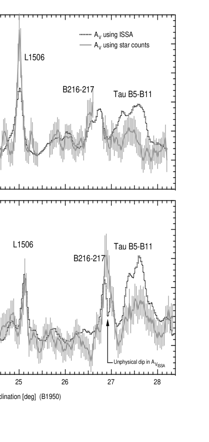
Figure 4: Plots of extinction vs. declination for both cut 1 and cut 2. The solid line is the extinction obtained through star counts. The dotted line is the extinction obtained using the ISSA 60 and 100 µm images. Both methods are averaged over the 10′ width of the cut. Breaks in the star count extinction trace are due to missing $R$-band frames. The error bars in the star count extinction represent the 1 $\sigma$ error. The rise in extinction associated with the dark clouds and IRAS cores are identified. The dip in the extinction peak associated with B216-217, in the $A_{V_{ISSA}}$ trace of cut 2 is due to an unreal drop in the extinction caused by the presence of IRAS point source in the images.

An interesting point to note is that several “elliptical holes” in the extinction appear in Figure 1. These “holes” are unphysical depressions in the extinction produced by the hot sources seen in the 60 µm maps. The 60 µm point sources (mostly embedded young stars) heat the dust around them and create a region where there is an excess of hot dust. This limitation, caused by the low spatial resolution of IRAS and assuming a single $T_{d}$, will then create an unphysically low extinction, when calculating the $A_{V}$ in the region near IRAS point sources, using the method described above. Unfortunately, cut 2 (see Figure 1) passes near two of these unphysically low extinction areas. (In Figures 4 and 5 we mark the position of the unreal dip in extinction.) These unphysical holes in $A_{V}$ are each associated with two very close IRAS point sources (one hole is produced by IRAS 0418+2654 and IRAS 0418+2655, and the other one by IRAS 0418+2650 and IRAS 0419+2650) inside the dark cloud B216-217 (see end of §3.2).

As mentioned above, in order to calculate the optical depth we assumed that the dust emissivity is proportional to a power law ($\tau_{d}\propto\lambda^{-\beta}$), with index $\beta=1$. Though studies differ in the values they find for $\beta$, there is a general agreement that the emissivity index depends on the grain’s size, composition, and physical structure (Weintraub et al. 1991). The general consensus in recent years has been that $\beta$ has a value most likely between 1 and 2, that in the general ISM $\beta$ is close to 2, and in denser regions with bigger grains, $\beta$ is closer to 1 (Beckwith & Sargent 1991; Mannings & Emerson 1994; Pollack et al. 1994). Our region of interest has both lines of sight that pass through low and high density medium with different environments. Thus, there is no way we can use a “perfect” or “preferred” value of $\beta$, as it might be different for different lines of sight. In our case we had to choose the same value as Jarrett et al. (1989) and Wood et al. (1994), which is $\beta=1$, since we use their results to convert from $\tau_{100}$ to extinction. The errors introduced by assuming a constant $\beta$ are hard to estimate, since we do not have any way to measure how much $\beta$ changes in our region of study. We do not include these errors in the error estimate of $A_{V}$ using ISSA images (from now on $A_{V_{ISSA}}$), but it must be kept in mind that $\beta$ is not necessarily equal to 1 and that its value may vary for different lines of sight.

In order to estimate the pixel-to-pixel (random) errors in $A_{V_{ISSA}}$, we examined a circular area of 800 pixels centered at 4h 19m, 22°24′ (B1950) which appears to have a constant extinction. We compared pixels that are 1.5 IRAS beams apart and obtained a standard deviation in the extinction value of this region to be 0.06 mag. We use this value as an estimate of the pixel-to-pixel errors in $A_{V_{ISSA}}$.

Ultimately, though, we need an estimate of the total error in $A_{V_{ISSA}}$, not just pixel-to-pixel errors. As explained above, the north and south extinction maps give slightly different extinction values for matching pixels in the region where they overlap. By fitting a gaussian to a histogram of the difference in $A_{V_{ISSA}}$ value between the north and the south extinction map, we find a $1\sigma$ width of 0.11 mag. We use this value as an estimate of the $1\sigma$ error in $A_{V_{ISSA}}$ caused by uncertainty in the zero level constants and zodiacal subtraction in the ISSA plates. Adding this “plate-to-plate” error in quadrature to the the pixel-to-pixel error (previous paragraph) gives a total error in $A_{V_{ISSA}}$ of 0.12 mag. We use this value as an estimate of the error in $A_{V_{ISSA}}$, but we remind the reader that this error does not include any errors caused by assuming a constant $\beta$.

3 Results

The data described above offer the opportunity to measure $A_{V}$ in four different ways: 1) using the 85 stars in cut 1 for which we have color excess data (see Table 1); 2) using 60 and 100 µm ISSA images as described in Section 2.4; 3) using star-counting techniques on the $R$-band frames; and 4) using an optical ($V$ and $R$) version of the average color excess method used by LLCB, described in more detail in Section 3.3.

Throughout the paper we assume that the extinction we calculate, independent of the way it was obtained, is produced by the dust associated with the Taurus dark cloud complex at a distance of 140 $\pm 10$ pc (Kenyon et al. 1994). The region of Taurus we observed lies at Galactic coordinate $l^{II}\approx 172\arcdeg$, $b^{II}\approx-17\arcdeg$. Thus, our stars lie towards lines of sight where there is little or no dust except for that associated with the Taurus dark cloud and, we can safely assume that in the area under study, virtually all the extinction is produced by the dust associated with the Taurus dark cloud complex.

3.1 Extinction from the color excess of stars with measured spectral types

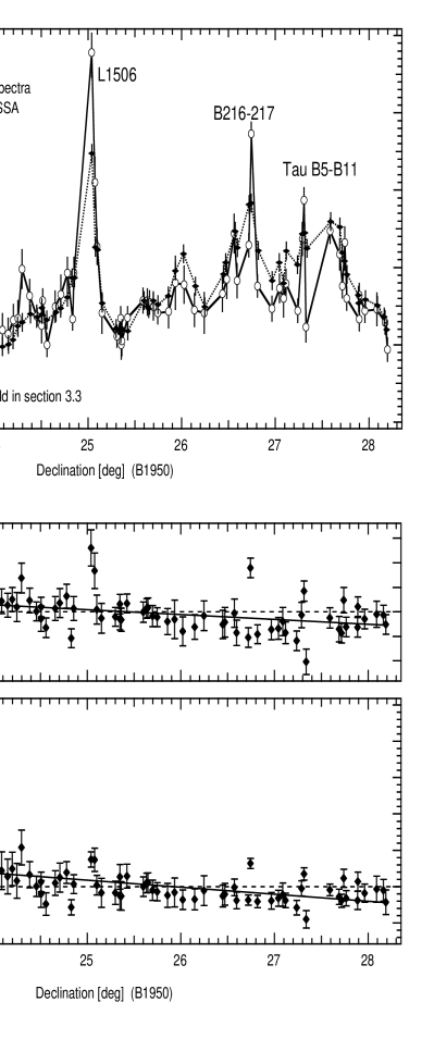
Figure 3: The top panel (Figure 3a) shows the extinction of every star we classified by spectral type with distances larger then 140 pc in cut 1, as well as the extinction at the same position on the sky using the ISSA extinction map (Figure 1). The error bars shown represent only the random erors for each of the two methods, systematic errors are not included. Also shown in Figure 3a is the region used as reference field for the extinction obtained using the technique described in section 3.3. Figure 3b shows the difference between the two different extinction values from Figure 3a. Figure 3c shows the difference (from Figure 3b) divided by the ISSA extinction ($A_{V_{ISSA}}$). The solid lines in Figures 3b and 3c are the unweighted linear fits to the points in each of the two plots. These lines indicate the small gradient in extinction with declination in $A_{V_{ISSA}}$, which we believe is due to an imperfect zodiacal light subtraction of the ISSA images.

Using the color excess and position data for the stars in Table 1 that lie on cut 1 and have a distance larger than 150 pc, we construct the extinction vs. declination plot shown in Figure 3a. This technique easily detects the rises in extinction associated with Tau M1 around Dec $23.65\arcdeg$, L1506 around Dec 25°, B216-217 around $26.7\arcdeg$, and the area near the IRAS cores Tau B5 and Tau B11 (hereafter Tau B5-B11) around Dec $27.5\arcdeg$. As in the ISSA $A_{V}$ map (Figure 1), the extinction obtained from the color excess of stars ($A_{V_{sp}}$) shows an overall rise in extinction with increasing declination. Also plotted in Figure 3a are the extinction values obtained from the ISSA extinction map ($A_{V_{ISSA}}$) for the same coordinates on the sky where there is a $A_{V_{sp}}$ point. The value of each $A_{V_{ISSA}}$ point is obtained from the pixel nearest to the coordinates of each star with measured $A_{V_{sp}}$ in cut 1. The error bars, set at $\pm 0.12$ mag for each $A_{V_{ISSA}}$ point, show the total error (including pixel-to-pixel and plate-to-plate variations, but not including systematic errors) discussed above.

As a check on the assumed value of $R_{V}$, we let $R_{V}$ vary in the calculation of $A_{V_{sp}}$ and then calculate $\Delta_{tot}=\Sigma^{N}_{i=1}|R_{V}E_{B-V}-A_{V_{ISSA}}|_{i}$ (where $i$ represents the $i$th point in the plot) for different values of $R_{V}$. We found that $R_{V}\sim 3.05$ minimizes the difference between the two curves ($\Delta_{tot}$). This reassures us that the choice of a constant $R_{V}=3.1$ is a good assumption.

The traces of $A_{V}$ vs. declination in Figure 3a show a very striking similarity. Although the beam size of ISSA is $\sim 5\arcmin$ and $A_{V_{sp}}$ has a beam, due to seeing effects, of approximately 3″ (which transform into 0.2 pc and 0.002 pc, respectively, at a distance of 140 pc), both values agree within the errors in most places. A plot of ($A_{V_{sp}}-A_{V_{ISSA}}$) vs. declination is shown in Figure 3b. It can be seen that $A_{V_{sp}}-A_{V_{ISSA}}\approx 0$, within errors, for all points not in the vicinity of a steep increase in extinction (i.e. away from dark clouds and IRAS cores). In other words, in the low extinction regions $A_{V_{sp}}$ is very similar to $A_{V_{ISSA}}$, despite the great difference in the resolution of the two methods. This leads us to believe that there are no or only very small fluctuations in the extinction inside a 5′ beam, in low $A_{V}$ regions. In order to put an upper limit to the magnitude of the fluctuations, we present a plot of $A_{V_{sp}}-A_{V_{ISSA}}$ divided by $A_{V_{ISSA}}$, in Figure 3c. We discuss this plot more in §4.1.

The gently sloping solid lines in Figures 3b and c are unweighted linear fits to the points in each of the plots. Both fits have a very small, but detectable, slope (0.1 mag/degree for Figure 3b). Previous studies using IRAS data have attributed the existence of gradients like these to imperfect zodiacal light subtraction (Wood et al. 1994). Moreover, the fact that the linear fit of the middle panel crosses the $A_{V_{sp}}-A_{V_{ISSA}}$ zero line at a declination of around 25.4°, near the middle of the overlap region between the northern and southern $A_{V_{ISSA}}$ (Figure 1) map, leads us to believe that the small gradient is due to imperfect ISSA image reduction. The gradient in $A_{V_{ISSA}}$ gives a pixel-to-pixel offset of 0.008 mag/beam, which is much less than the pixel-to-pixel random errors in $A_{V_{ISSA}}$, and much, much less than other systematic errors (e.g. constant $\beta$) so we do not to correct for it.

3.2 Star counting

With the help of IRAF, as described in §2.1, we located a total of 3,715 stars in cut 1 and 3,074 stars in cut 2, with $14.5\leq m_{R}<18.0$, from the November 1995 $R$-band images. With this database of stellar positions we measure the extinction over the region covered by both cuts, using classical star counting techniques. First, we subdivide each cut into a rectilinear grid of overlapping squares, and then we count the total number of stars in each square. Our ultimate goal in star counting is to obtain the extinction of the region in a way that can be compared to the other techniques used in this paper. Therefore, in order to mimic the resolution and sampling frequency of the ISSA data, we made the counting squares 5′ on a side (the resolution of ISSA) and the centers of the squares were separated by 1.5′ (the size of an ISSA pixel).

Conventionally, measuring extinction from star counts involves comparing the integrated number of stars within a given cell towards the region of interest to a nearby reference field which is assumed to be free from extinction (Bok & Cordwell 1973). Several assumptions need to be made in order to use this method: 1) the population of stars background to the region of interest does not vary substantially and is similar to the reference field; 2) the extinction ($A$) is uniform over the count cell; and 3) the integrated surface density of stars for the reference field ($N_{ref}$) of stars brighter than the apparent magnitude, $m$, follows an exponential law with ${\rm log}(N_{ref}(<m))=a+bm$. The integrated surface density of stars for any other field under study, $N_{on}$, follows a similar law, ${\rm log}(N_{on}(<m))=a+b(m-A)$.

In our case, the extinction to each square was obtained via:

$$A_{V_{on}}=A_{V_{ref}}+\frac{A_{V}}{A_{R}}\frac{{\rm log}(n_{ref}/n_{on})}{b_{R}}$$ (7)

where $A_{V_{ref}}$ is the extinction of the reference field, $n_{ref}$ is the number of stars in the reference field, and $n_{on}$ is the number of stars in any of the other counting cells. The quantity $b_{R}$ is the slope of the cumulative number of stars as a function of $R$ apparent magnitude (see assumption 3 in previous paragraph). We calculate $b_{R}$ by fitting a line to ${\rm log}(N_{ref}(<m_{R}))$ for $14.5\leq m_{R}<18.0$, and obtain a value of $0.34\pm 0.02$. The ratio $A_{V}/A_{R}$ is the reddening law between $V$ and $R$ wavelengths, which gives the value of 1.24 (He et al. 1995) used in the conversion for star counts in (Cousins) $R$ to extinction in $V$.

As mentioned above, in conventional star count studies, the reference fields are areas in the sky, close to the region under study, which have $A_{V_{ref}}=0$. This is not so in our case. Since our CCD data were not originally obtained for star counting purposes, we did not take any images of a reference field with $A_{V_{ref}}=0$. Thus, the reference fields were chosen to be regions where we could safely assume the value of $A_{V_{ref}}$. Specifically, the reference fields were chosen by virtue of their having a spectroscopic probe star to which we derived the extinction through its color excess.

One of the major assumptions in conventional star counting studies is that the population of background stars to the cloud is similar to that in the reference field. This is why star count studies are only done over small regions of the sky. In our case, cut 1 (the longer cut) expands 6 degrees in declination which transforms to nearly 4° in Galactic latitude ($-18.8\arcdeg<b^{II}<-14.9\arcdeg$). This span in Galactic latitude is enough to have a big effect on the surface density of stars due to galactic variations; one detects more stars per cell, for a constant $A_{V}$, the closer one observes to the galactic plane. (The star count Galaxy model of Reid et al. [1996] predicts that a 10 square degree field with no extinction centered at $b^{II}=-14\arcdeg$, $l^{II}=-172\arcdeg$ will have approximately a factor of two more stars than a 10 square degree field with no extinction centered at $b^{II}=-19\arcdeg$, $l^{II}=-172\arcdeg$.) Thus, it was imperative that we correct for Galactic changes in the stellar density. Not doing this would have resulted in an unreal drop in the derived extinction for lower Galactic latitudes. We account for the Galactic gradient by using 4 different, more or less evenly spaced, reference fields at different galactic latitudes along the cut. Each of these fields has a star with measured reddening (from Table 1) which was used to estimate the extinction of the reference field in question. Thus, for example, the star count extinction located between $b^{II}=-18.9\arcdeg$ and $b^{II}=-17.9\arcdeg$ (which transforms to $22\arcdeg 25\arcmin<\delta_{J2000}<23\arcdeg 56\arcmin$ in cut 1) is tied to the reference field where star 011001 lies; the star count extinction in the region with $-17.9\arcdeg\leq b^{II}<-16.9\arcdeg$ (which transforms to $23\arcdeg 56\arcmin<\delta_{J2000}<25\arcdeg 25\arcmin$ in cut 1) is tied to the reference field where star 051043 lies; and so forth. The number of stars ($n_{ref}$), the visual extinction ($A_{V_{ref}}$), and the range in $b^{II}$ which each of the four reference fields calibrates are given in Table 3. It is important to stress that by doing this calibration we are tying $A_{V_{sc}}$ to $A_{V_{sp}}$ at these four points, and thus $A_{V_{sc}}$ is not totally independent of $A_{V_{sp}}$. But this procedure only forces $A_{V_{sc}}$ to agree in absolute value to $A_{V_{sp}}$ in four points and not to give the same structure or scale through the cuts.

In our study, where observations lie primarily along a declination cut, the best way to graphically compare the extinction measured by star counting ($A_{V_{sc}}$) and from the ISSA images ($A_{V_{ISSA}}$) is to plot them both in an extinction versus declination plot. (Cut 1 is about 6 degrees long, but only 10′ wide, giving a ratio of 1:36 between length and width. This makes it practically impossible to show a legible figure of a star count extinction map of the cuts.) A value of the extinction was obtained for each $5\arcmin\times 5\arcmin$ counting box, and then averaged extinction over R.A. for every point in declination, so as to produce only one value of $A_{V}$ for each declination, independent of R.A. Constant declination slices every 5′ show that the variations in $A_{V_{ISSA}}$ across the 10′ width of each cut are not large. Most of the constant declination slices had standard deviations in $A_{V_{ISSA}}$ of less than 0.2 mag, and none exceeded 0.3 mag. Moreover, most adjacent counting boxes, with the same declination, differ in $A_{V_{sc}}$ by less than 0.2 mag. Therefore, we are confident that we are not introducing large errors by averaging the extinction over the $\sim$ 10′ spanned by each cut in Right Ascension. On the other hand, by averaging over R.A., the sensitivity to small scale fluctuations decreases. The smoothed (averaged) extinction trace has less sensitivity in detecting fluctuations on 5′ scales than on 10′ scales, where it reaches full sensitivity. Nevertheless, averaging the extinction over R.A. does not create any disadvantage for the purpose of comparing the different ways of calculating the extinction since all the techniques are averaged over the same width.

Figure 4 shows $A_{V_{sc}}$ and $A_{V_{ISSA}}$ (now both averaged over the $\sim$ 10′ that spanned each cut in R.A.) versus declination, for both cuts. The random errors in the star count trace are plotted for each point. The uncertainty in the number of stars in each sampling box is given by $\sqrt{n}$ (Poisson statistics), where $n$ is the number of stars counted in the box (Bok 1937). The uncertainty in the extinction (with contributions from the uncertainty in $n$, $n_{ref}$, $A_{V_{ref}}$, and $b_{R}$) for each sampling box with the same declination is then averaged to give the final (plotted) error in the extinction. Like the ratio of total-to-selective extinction ($R_{V}$), the value of $A_{V}/A_{R}$ may vary from one line of sight to the other. Also, like $R_{V}$ in section 2.2, here we use the ISM average value of $A_{V}/A_{R}$. We do not take the errors caused by assuming a constant value of $A_{V}/A_{R}$ into account when we calculate the errors in $A_{V_{sc}}$, as we have no way of calculating them.

It can be seen that both $A_{V_{ISSA}}$ and $A_{V_{sc}}$ show the same gross extinction structure. Both have local maxima and minima in the same places (in most cases), but not at necessarily the same value. Both traces detect rises in extinction associated with Tau M1, L1506, B216-217, and Tau B5-B11. It is clear that $A_{V_{sc}}$ has more fluctuations than the $A_{V_{ISSA}}$ trace. These fluctuations are not likely to be real, as most of them are of the same magnitude as the errors in $A_{V_{sc}}$. Most of the “noise” in the extinction is due to the fact that the star count technique is very dependent on the assumption of a constant background stellar surface density. Real (small) changes in the background surface density of stars (not caused by extinction) will produce unreal fluctuations in the resultant $A_{V_{sc}}$.

Note the unreal dip in the cut 2 trace of $A_{V_{ISSA}}$ (see Figure 4), caused by assuming a constant dust temperature for those lines of sight where there are IRAS point sources which heat the dust around them (see section 2.3). This shows the potentially large errors in $A_{V_{ISSA}}$ that can arise from assuming a single dust temperature ($T_{d}$) for each line of sight. The other place where there is a significant discrepancy between $A_{V_{ISSA}}$ and $A_{V_{sc}}$ is in the rise in extinction associated with Tau B5-B11 (see Figure 4), where the two methods disagree by more than $1\sigma$ of the error in $A_{V_{sc}}$. This discrepancy will be discussed further in §4.2.

3.3 Extinction measured via average color excess method

Taking advantage of the fact that we had taken our November 1995 images in more than one broad band filter, we used the method developed by LLCB to study the extinction along both cuts in yet another way. This method consists of assuming that the color distribution of stars observed all along the cut is identical in nature to that of stars in a control field. With this assumption one can use the mean $V-R$ color of the stars in the control field to approximate the intrinsic $V-R$ color of all stars background to the cloud. (Note that LLCB’s analysis was in the near-infrared, and they used $H-K$ colors—which have even less intrinsic variation than $V-R$ colors.) Using the same technique as in star counting, the region under study is divided into a grid of overlapping counting boxes, and then an average of the color excess (and extinction) of the stars in each counting box is obtained.

To derive extinction from the average color excess method, we used the same sample of stars, with $14.5\leq m_{R}<18.0$, used in our star counting study (§3.2). The region between declinations 22.9° and 23.22° (B1950) was used as our reference field since, as can be seen in Figure 3a, this region has a uniform extinction within the errors. We took an average of the extinction of the 6 stars for which we had spectral types and which lie inside this region, and obtained a value of $A_{V_{ref}}=0.72\pm 0.2$. We did not divide the area under study into square sampling boxes as it is usually done in star count studies (see previous section). Instead, the area under study was divided into rectangular cells, where the R.A. side of the rectangle was dictated by the frames’ width ($\sim 10\arcmin$) and the declination side was set to be 5′. The centers of the rectangles were separated in declination by 1.5′. This was done in order to keep the same resolution and sampling frequency in the declination direction as in the ISSA and star counting methods (described in the previous sections). We are not sensitive to any variations in extinction within each measurement rectangle, but Figure 3a suggests that such variations are very small.

The number of stars in each rectangle was counted and the color excess of each star was obtained using the formula:

$$E_{V-R}=(V-R)-\langle V-R\rangle_{ref}$$ (8)

where $\langle V-R\rangle_{ref}$ is the mean V R color of the reference field, which in our case is $0.60\pm 0.05$ mag. Figure 5 shows the distribution of V R colors in the reference field. We then apply equation 8 to each star in a counting rectangle and obtain a mean color excess to each rectangle:

$$\langle E_{V-R}\rangle={\frac{\Sigma_{i}^{N}(E_{V-R})_{i}}{N}}$$ (9)

where $N$ is the number of stars in a counting rectangle and $(E_{V-R})_{i}$ is the color excess of the $i$th star. The mean visual extinction is obtained using:

$$\langle A_{V}\rangle=A_{V_{ref}}+{\frac{A_{V}}{E_{V-R}}}\times\langle E_{V-R}\rangle$$ (10)

where $A_{V_{ref}}$ is the extinction of the reference field (0.72 mag), and we use the ISM average value of 5.08 for the expression $A_{V}/E_{V-R}$ (He et al. 1995). Similar to the extinction from star counts, the extinction using the average color excess (from now on $A_{V_{ce}}$) is not totally independent of the spectral classification method. Recall that $A_{V_{ref}}$, which is used to calibrate $A_{V_{ce}}$,is determined using measurements of $A_{V_{sp}}$. This calibration forces $A_{V_{ce}}$ to agree in absolute value with the average of $A_{V_{sp}}$ in the reference field, but it does not force $A_{V_{ce}}$ to give the same structure or scale in the extinction curves throughout the cuts.

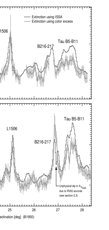
Figure 6: Similar to Figure 4, but this time the solid line is the extinction obtained through the average color excess method described in §3.3. Breaks in the solid line trace in cut 1 are due to missing $R$-band frames. The error bars in the average color excess extinction represent the 1 $\sigma$ error. The dip in the extinction peak associated with B216-217, in the $A_{V_{ISSA}}$ trace of cut 2 is due to an unreal drop in the extinction caused by the presence of IRAS point source in the images.

Using the average color excess technique, we are able to detect the same overall trends in extinction found from the ISSA plates, spectral analysis, and star counting (see Figure 6). The rises in extinction due to Tau M1, L1506, B216-217, and Tau B5-B11 can be seen as well pronounced peaks in $A_{V}$. Again, note the unreal dip in the cut 2 trace of $A_{V_{ISSA}}$, caused by the presence of four IRAS point sources in the dark cloud B216-217 (see section 2.3). In Figure 6 we also show the random errors of each point in the $A_{V_{ce}}$ trace. The measurement uncertainty in $A_{V_{ce}}$ for any given counting cell is given by:

$$\sigma_{A_{V_{ce}}}=\sqrt{\sigma_{ref}^{2}+(5.08)^{2}[\sigma^{2}_{mean}+\Sigma_{1}^{N}\frac{\sigma^{2}_{(V-R)_{i}}}{N^{2}}]}$$ (11)

where $\sigma_{ref}$ is the uncertainty in $A_{V_{ref}}$ (which is equal to 0.2 mag), $N$ is the number of stars in the counting cell and $\sigma_{(V-R)_{i}}$ is the photometric error in $V-R$ of the $i$th star inside the cell. The quantity $\sigma_{mean}$ is the error in the mean of the $V-R$ color distribution of the counting cell. The distribution of the $V-R$ colors does not have a gaussian distribution, thus $\sigma_{mean}$ was obtained using Monte Carlo simulations. We obtained $N_{mc}$ values of $V-R$, representing the $V-R$ colors of $N_{mc}$ stars in a counting cell, drawn from a distribution given by the reference field distribution (Figure 5). We then computed the average $V-R$ color over these $N_{mc}$ stars. The procedure was repeated a thousand times with the same $N_{mc}$, from which we obtained a (gaussian) distribution of average values. The 1$\sigma$ width of this gaussian was then used as the value of $\sigma_{mean}$. This procedure was repeated for different values of $N_{mc}$ (representing different number of stars inside a counting cell). We do not include the errors in $A_{V_{ce}}$ caused by assuming a constant $A_{V}/E_{V-R}$ for all lines of sight.

Although $A_{V_{ce}}$ and $A_{V_{ISSA}}$ agree very well for the low declination ($\delta<25.5\arcdeg$) part of both cuts, their values seem to diverge for higher declinations ($\delta>25.5\arcdeg$; Figure 6). This effect suggests that it may be inappropriate to assume a single average color for the whole length (6°) of our cuts. A change in the average V R could be due to: 1) a gradient in the $\langle V-R\rangle$ caused by a greater fraction of early type stars close to the galactic plane; and/or 2) a sudden drop in the value of $\langle V-R\rangle$ in the north edge of the cuts due to the presence of a star cluster. Concerning the first point, the star count Galaxy model of Reid et al. (1996) predicts that a 10 degree square degree field with no extinction centered at $b^{II}=-14\arcdeg$, $l^{II}=172\arcdeg$ will have approximately an average star ($V-R$) color 0.04 mag greater than a 10 degree square degree field with no extinction centered at $b^{II}=-19\arcdeg$, $l^{II}=172\arcdeg$. A difference of 0.04 mag in $\langle V-R\rangle$ transforms to a difference of 0.2 mag in $A_{V_{ce}}$. Thus, it is possible that at least some of the discrepancy between $A_{V_{ce}}$ and $A_{V_{ISSA}}$ for the northern parts of both cuts is due to this uncorrected effect of varying $\langle V-R\rangle$. We will discuss the possibility of a cluster in section 4.3.

4 Analysis and Discussion

4.1 Structure in the cloud

Figure 3a shows a striking resemblance between the extinction obtained through the use of the ISSA 60 and 100 µm images ($A_{V_{ISSA}}$) and the extinction obtained through the color excess of individual stars which we had classified by spectral type ($A_{V_{sp}}$). Our stellar reddening (color excess) sample represents a map of the distribution of extinction ($A_{V_{sp}}$) which, although it has a “pencil beam resolution,” is measured in a spatially nonuniform fashion. On the other hand the extinction data obtained from the ISSA images is spatially continuous, with 1.5′ pixels and a resolution of 5′ ($\sim 0.2$ pc at a distance of 140 pc). Most stars with measured $A_{V_{sp}}$ are less than 5′ from their nearest star with measured $A_{V_{sp}}$, and there are a number of cases where three and even four stars lie within 5′ of each other. Therefore if one were to place a 5′ beam anywhere along cut 1, one would find that 1 to 4 stars would lie, in random places, inside the beam. Thus, if there were to exist big fluctuations in the dust distribution inside the 0.2 pc beam of IRAS, we would see strong variations between the value of $A_{V_{sp}}$ and the value of $A_{V_{ISSA}}$. Note that this fluctuation probe can only be used where there are stars that have been classified by spectra.

Using the extinction measurements shown in Figure 3, we can place an upper limit on the fluctuations in the dust distribution within a 5′ beam. In the bottom panel of Figure 3c we plot the difference between $A_{V_{sp}}$ and $A_{V_{ISSA}}$ divided by $A_{V_{ISSA}}$ (from now on $\Delta A_{V}/A_{V}$) versus declination. Here the errors are obtained using the quoted errors for $A_{V_{sp}}$ (see Table 1) and $A_{V_{ISSA}}$ (0.12 mag), and propagation of errors. One can think of $\Delta A_{V}/A_{V}$ as a measurement of the deviations in the average extinction within a fixed area of the sky. In our case the area is given by the 5′ beam of $A_{V_{ISSA}}$.

Figure 3c has only four points with an absolute value which is more than 3 times its 1 $\sigma_{i}$ error (independent of whether we correct for the small gradient in $A_{V}$ with declination), where $\sigma_{i}$ is the error of each individual point on Figure 3c. Each of these four points is associated with one of the extinction peaks created by dark clouds and IRAS cores intersecting the cut. The high values of $\Delta A_{V}/A_{V}$ could be due to two effects indistinguishable by our data; spatially unresolved steep gradients in the extinction or random fluctuations in the dust distribution inside dark clouds and IRAS cores. These possibilities will each be discussed later. All of the remaining lines of sight, in the more uniform extinction areas, have absolute values of $\Delta A_{V}/A_{V}$ which are less than 3 times their 1 $\sigma_{i}$ error. If we exclude points near dramatic extinction peaks (see Figure 3), then we do not detect any deviations from zero in $\Delta A_{V}/A_{V}$ within our sensitivity.

We can characterize our sensitivity to extinction fluctuations using the average error in $\Delta A_{V}/A_{V}$, which is given by $\sigma_{av}=\Sigma_{i}^{N}\sigma_{i}/N$. The 1-$\sigma_{av}$ error in $\Delta A_{V}/A_{V}$, for points with $A_{V_{ISSA}}<0.9$ mag is 0.41, while for points with $A_{V_{ISSA}}\geq 0.9$ is 0.15. We choose $A_{V_{ISSA}}=0.9$ as the dividing line since points with $A_{V_{ISSA}}<0.9$ mag have consistently large uncertainties. Assuming that 0.15 is the “typical” error in $\Delta A_{V}/A_{V}$ for points with $A_{V_{ISSA}}\geq 0.9$, we can then state that a real detection (using a 3-$\sigma_{av}$ detection limit) of sub-IRAS beam structure would be if $\Delta A_{V}/A_{V}\gtrsim 0.45$. Therefore only in places where $\Delta A_{V}/A_{V}>0.45$, can we say that there are sub-IRAS beam structures in the cloud. Any value less than 0.45 would be considered part of the “noise” and not significant enough to be considered a detection of sub 0.2 pc structure. So, ultimately, we only detect deviations from the mean $A_{V}$ within a 0.2 pc beam in the vicinity of IRAS cores and dark clouds. Outside of those regions, deviations within a 0.2 pc beam are limited to be less than $\Delta A_{V}/A_{V}<0.45$ (for $A_{V}>0.9$). For points with extinction less than 0.9 mag the larger uncertainty in the extinction determinations means that only points with $\Delta A_{V}/A_{V}\gtrsim 1.23$ would be real fluctuations detections, and no such points are found.

4.2 Evidence for smooth clouds

In a very important study, Lada et al. (1998; hereafter LAL) recently showed that smoothly varying density gradients can produce the “fluctuations” observed in extinction studies of filamentary clouds. Two studies of dust extinction in filamentary dark clouds had been conducted previous to LAL: 1) the study of IC 5146 by LLCB; and 2) a study of L977 by Alves et al. (1998). Both studies find that in $1.5\arcmin\times 1.5\arcmin$ cells, the dispersion of extinction measurements within a square map pixel (what LLCB name $\sigma_{disp}$) increases in a systematic way with the average $A_{V}$, in the range of $0<A_{V}<25$ mag. Both studies conclude that the systematic trend in their $\sigma_{disp}-A_{V}$ plot, an increase of $\sigma_{disp}$ with $A_{V}$, is due to variations in the cloud structure on scales smaller than the resolution of their measurements. But neither of the studies could definitively determine the nature of the fluctuations in the extinction. This prompted LAL to study IC 5146 in the same way as LLCB, but at a higher spatial resolution (30″). With the help of Monte Carlo simulations LAL conclude that the form and slope of the $\sigma_{disp}-A_{V}$ relation, and hence most (if not all) of the small scale variations in the extinction are due to unresolved gradients in the dust distribution within the filamentary clouds. LAL note that random spatial fluctuations in the dust distribution could exist, at a very low level, in addition to the smooth gradients. They state that $\sigma_{ran}/A_{V}$ due to random fluctuations is much less than 25% at $A_{V}\sim 30$ mag, which is consistent with our ($3\sigma$) upper limit of $\Delta A_{V}/A_{V}=0.45$ at $0.9<A_{V}<3.0$ mag.

Recently, Thoraval et al. (1997), hereafter TBD, observed a low $A_{V}$ area of the IC 5146 dark cloud complex. Similar to our study, TBD concentrate their observations in a low and uniform extinction region ($A_{V}<5$), but unlike our study, the region that TBD studied did not include a filamentary cloud. They conclude that the variations in the extinction are present at a level no larger than $\Delta A_{V}/A_{V}\sim 0.25$, again consistent with our ($3\sigma$) upper limit of $\Delta A_{V}/A_{V}=0.45$, and similar to what LAL obtain in the high extinction region of IC 5146. If we exclude, in our study, the points near extinction peaks, we are left with the same results as TBD: no fluctuations on scales smaller than the resolution. These results all suggest that there is very little random spatial fluctuation in the extinction in regions of low $A_{V}$ far from extinction peaks.

Although it is not possible to definitively determine the origin of the handful of high $\Delta A_{V}/A_{V}$ we find near extinction peaks, it is more likely that they are due to unresolved steep gradients in clouds than to localized random fluctuations in the dust distribution. The filamentary dark clouds and IRAS cores typically have a minor axis that is only 3 to 4 times the IRAS beam size, so some IRAS beam will undoubtedly contain a steep extinction gradient characterizing the the “edge” of one of these structures. Extinction measurements using a pencil-beam (e.g. $A_{V_{sp}}$), would be able to resolve this “edge,” so, near edges, large-beam (e.g. $A_{V_{ISSA}}$) and pencil-beam measurements would disagree. The results of TBD and LAL reinforce this hypothesis. Thus, we strongly believe that the high values of $\Delta A_{V}/A_{V}$ near dark clouds and IRAS cores are due to steep gradients in the extinction not resolved by the IRAS beam.

4.3 Possible discovery of a previously unknown cluster

While comparing our different ways of obtaining the extinction we found a peculiar discrepancy between $A_{V_{ISSA}}$ and $A_{V_{sc}}$ and between $A_{V_{ISSA}}$ and $A_{V_{ce}}$, in the declination range from 27.2° to 28° (B1950) along the two cuts (see Figure 4). The rise in ISSA extinction in these declinations is due to the existence of a high dust concentration which Wood et al. (1994) classify as the IRAS cores Tau B5 and Tau B11 (Tau B5-B11). The trace of $A_{V_{ISSA}}$ shows that the increase in the extinction associated with Tau B5-B11 is of similar or higher magnitude to the increase in extinction associated with the dark cloud B216-217, in both cuts (see Figure 6). On the other hand, the star count extinction and the average color excess extinction show a small increase in $A_{V}$ associated with Tau B5-B11 compared to that associated with B216-217. In addition, there is no sharp decrease in the surface density of stars like the one associated with the two dark clouds in our cuts. This can be observed in both the spatial distribution of our $R$-frame stars and in the Digitized Palomar Sky Survey.

One possible explanation for the discrepancy between extinction traces is that either $A_{V_{ISSA}}$ or $A_{V_{ce}}$ and $A_{V_{sc}}$ were calculated using the wrong assumptions. It could be that the dust in the Tau B5-B11 region has different physical properties compared to the rest of the dust in the Taurus dark cloud complex, which would change the values of $\beta$ or of $A_{V}/A_{R}$ and $A_{V}/E_{V-R}$. When we calculated $A_{V_{ISSA}}$, $A_{V_{sc}}$, and $A_{V_{ce}}$, we assumed that the power law index, $\beta$ (equation 4), $A_{V}/A_{R}$ (equation 7) and $A_{V}/E_{V-R}$ (equation 10) were constant for all lines of sight. We could change the value of $A_{V}/A_{R}$ (equation 7) from 1.24 to 1.74 in order for $A_{V_{sc}}$ to be approximately equal to $A_{V_{ISSA}}$ for the lines of sight that pass through Tau B5-B11. But, the value of $A_{V}/A_{R}$ is tied to the value of $A_{V}/E_{V-R}$, by the equation ${\frac{A_{V}}{E_{V-R}}}={\frac{1}{1-{\frac{A_{R}}{A_{V}}}}}$, thus the proposed change in $A_{V}/A_{R}$ would change $A_{V}/E_{V-R}$ from 5.08 to 2.35, making the discrepancy between $A_{V_{sc}}$ and $A_{V_{ISSA}}$ (Figure 6) more pronounced. An alternate possibility is that the value of $\beta$ changes from 1 to a value less than 1 for lines of sight in the region of Tau B5-B11, in that case $A_{V_{ISSA}}\approx A_{V_{sc}}\approx A_{V_{ce}}$. Although it is possible to have neighboring lines of sight with different dust properties, it is very unlikely (but not impossible) to have dust with $\beta<1$ in a region like Tau B5-B11, according to experimental and theoretical studies of dust properties (Weintraub et al. 1991; Pollack et al. 1994).

A more likely explanation for the discrepancy between extinction traces near Tau B5-B11 is that there is a sharp increase in the stellar distribution in the area, which we did not account for when we calculated $A_{V_{sc}}$. The existence of a previously unknown stellar cluster in the vicinity of R.A. 4h 19m, Dec. $27\arcdeg 30\arcmin$ (B1950) could create such an increase in the number of stars in the region. Also, if the cluster is relatively young, the average stellar colors should be bluer than in the field. This can explain why the $A_{V_{ce}}$ trace follows, within the error, the structure present in the $A_{V_{ISSA}}$ trace, but at a lower value, while the $A_{V_{sc}}$ trace decreases in extinction value without following the structure in $A_{V_{ISSA}}$.

We conclude that there is a sudden increase in the stellar distribution background to Tau B5-B11 (and a change in the average V R color), which is due to a previously unknown open star cluster. This is more credible than a change in dust properties, since the cluster hypothesis does not require the assumption of a physically contradictory, simultaneous change in the value of $A_{V}/A_{R}$ and $A_{V}/E_{V-R}$, or an improbable value of $\beta$. We expect that further observations of the area will verify the existence of an open cluster behind Tau B5-B11.

5 Rating the Various Methods

Although we find that all four methods give generally similar results and are consistent with each other, there are some important exceptions. The discrepancies arise from different systematic errors inherent to the different techniques. For example, when calculating $A_{V_{ISSA}}$, a constant dust temperature for each line of sight was assumed. This single temperature assumption breaks down in the immediate vicinity of stars surrounded by dust. Even though it is very likely that there is dust of many different temperatures along the lines of sight to these stars, it is the hot dust that dominates the emission at 60 and 100 µm, resulting in an incorrect estimate of $\tau_{100}$ (and $A_{V_{ISSA}}$), as we observe in the regions near IRAS sources.

The techniques that use background stellar populations to measure the extinction (i.e, star count and the average excess color method) also suffer from important systematic errors. Here the major systematic error lies in assuming a constant stellar population background to the cloud. If the region under study spans several degrees in galactic latitude (which is our case) uncorrected gradients in the background stellar density and the average stellar color will lead to incorrect extinction measurements when using for the star count method and the average excess color method, respectively. In addition, small fluctuations in the background surface stellar density can result in unreal fluctuations in the extinction.

It is important to appreciate that the techniques used in this Paper are not entirely standalone or independent methods of obtaining extinction. Even the most exact method for measuring extinction, using the color excess of individual stars with measured spectral type ($A_{V_{sp}}$) still depends on the value of $R_{V}$. Both star counting ($A_{V_{sc}}$) and the average color excess ($A_{V_{ce}}$) technique depend on a reference field of known extinction for calibration. In this study, $A_{V_{sc}}$ and $A_{V_{ce}}$ are calibrated using measurements of $A_{V_{sp}}$ in chosen reference fields, which means that $A_{V_{sc}}$ and $A_{V_{ce}}$ are then not completely independent of $A_{V_{sp}}$. Note though, that the calibration procedures only force methods to agree at a limited number of points, and it does not force them to have the same structure or scale through the cuts. $A_{V_{ISSA}}$ depends on a conversion from dust opacity at 100 µm to visual extinction, which ultimately relies on star count data in Jarrett et al. (1989). Thus, $A_{V_{ISSA}}$ is independent of any of the other extinction methods in this study, but it is tied to the star count data of Jarrett et al. (1989).

Table 4 outlines the advantages and disadvantages, and the random and systematic errors, of each of the four different methods of measuring extinction used in this Paper.

In principle, it would seem that the best method to calculate extinction is using the color excess of individual stars with measured spectral type, but this method is not without problem. One inconvenience is the fact that $R_{V}$ could have different values for different lines of sight. But systematic errors due to unknown constants are also present in the other methods ($\beta$ for $A_{V_{ISSA}}$, $A_{V}/A_{R}$ for $A_{V_{sc}}$, and $A_{V}/E_{V-R}$ for $A_{V_{ce}}$). Therefore not knowing the specific value of $R_{V}$ for every line of sight observed is not a disadvantage over the other methods. The real drawback of this technique is the large amount of time required to measure each and every star’s spectrum. Thus, although using the color excess of background stars with known spectral type is the most direct and accurate way of measuring the extinction, it is a very time consuming procedure and it measures the extinction in a spatially nonuniform fashion.

To asses the robustness of the four methods of measuring extinction used in this Paper, we constructed plots of $A_{V_{ISSA}}$, $A_{V_{sc}}$, and $A_{V_{ce}}$ versus $A_{V_{sp}}$, at each point where all four methods can be used. We do this in order to obtained a least square fit for each of the three remaining methods plotted against $A_{V_{sp}}$. The four points with the highest extinction were not included in the fits, since these are points near the extinction peaks of dark clouds. It is clear that for these four points $A_{V_{sp}}$ is larger than any of the other 3 methods since the 5′ beam of the other methods does not resolve the extinction gradients in this regions of high extinction (see section 4.1). When we constrain the fits to have a zero intercept, we find a slope of one (within the errors) in all three comparisons. Thus, we believe all four methods of obtaining extinction are robust.

6 Summary and Conclusions

We studied the extinction of a region of Taurus in four different ways: using the color excesses of background stars for which we had spectral types; using the ISSA 60 and 100 µm images; using star counting; and using an optical ($V$ and $R$) version of the average color excess technique of (Lada et al. 1994). All four give generally similar results. Therefore, any of the methods discussed above can be used to obtain reliable information about the extinction in regions where $A_{V}\lesssim 4$ mag.

We inter-compared the ISSA extinction and the extinction measured using individual stars, to study the spatial fluctuations in the dust distribution. Excluding areas where there are extinction gradients due to filamentary dark clouds and IRAS cores, we do not detect any variations in the structure on scales smaller than 0.2 pc. With this result we are able to place a constraint on the magnitude of the fluctuations. We conclude that in the regions with $0.9<A_{V}<3$ mag, away from filamentary dark clouds and IRAS cores, there are no fluctuations in the dust column density greater than 45% (at the 99.7% confidence level), on scales smaller than 0.2 pc. On the other hand, in regions of high extinction in the vicinity of dark clouds and IRAS cores, we do detect statistically significant deviations from the mean in dust column density on scales smaller than 0.2 pc. Although it is not possible to definitively determine the nature of the fluctuations with our data alone, the results of other studies (Lada et al. 1998, Thoraval et al. 1997) and ours taken together strongly favor unresolved steep gradients in clouds over random fluctuations on the dust distribution.

A discrepancy between the extinction obtained through star counting and average color excess and the rest of the techniques in the vicinity of R.A. 4h 19m, Dec. 27°30′ (B1950), leads us to believe in the existence of a previously unknown open stellar cluster in the region.

Table 1: Photometric and Spectroscopic Data

Star	R.A.	Dec	V	$\sigma(V)$	B V	$\sigma(\bv)$	Spectral	$E_{B-V}$	$A_{V}$	$\sigma(A_{V})$	distance	$\sigma(d)$
Name	(J2000)	(J2000)	[mag]	[mag]	[mag]	[mag]	Type	[mag]	[mag]	[mag]	[pc]	[pc]
011005	4h22m39.3s	22°28′08″	14.94	0.02	0.58	0.03	F2	0.23	0.73	0.16	1669	261
011003	4 22 38.5	22 38 47	16.57	0.02	0.97	0.04	G8	0.24	0.75	0.22	1156	291
011001	4 22 35.5	22 45 39	14.87	0.02	0.62	0.03	F6	0.16	0.51	0.16	1295	202
021015	4 22 35.5	22 48 02	15.99	0.02	0.83	0.03	F8	0.31	0.97	0.18	1459	235
021014	4 22 36.2	22 53 01	15.81	0.02	1.07	0.03	G8	0.34	1.05	0.21	711	177
021013	4 22 36.9	22 57 46	15.41	0.02	0.69	0.06	F6	0.23	0.72	0.23	1511	262
021012	4 22 39.5	23 03 30	14.94	0.02	0.71	0.03	F7	0.21	0.64	0.16	955	149
021011	4 22 36.3	23 05 39	15.18	0.02	0.74	0.03	F7	0.24	0.73	0.16	1231	192
00N5.2	4 22 34.4	23 08 09	14.40	0.02	0.58	0.02	F3	0.21	0.65	0.15	1292	199
031025	4 22 33.4	23 10 38	15.37	0.02	0.84	0.03	G0	0.26	0.81	0.18	1075	263
031024	4 22 29.7	23 12 54	15.47	0.02	0.90	0.03	G4	0.26	0.79	0.19	861	212
031023	4 22 29.7	23 16 11	15.23	0.02	0.69	0.03	F6	0.23	0.70	0.16	1398	219
031022	4 22 29.9	23 19 32	16.34	0.02	0.94	0.03	F9	0.39	1.21	0.18	1462	236
TDC071	4 22 22.5	23 20 07	15.60	0.02	0.54	0.03	A9	0.27	0.82	0.17	2720	434
041035	4 22 33.7	23 28 24	14.57	0.04	0.78	0.07	F7	0.28	0.86	0.25	877	158
TDC085	4 22 18.6	23 33 10	16.25	0.05	0.81	0.07	F6	0.34	1.07	0.25	1884	342
041033	4 22 33.6	23 37 38	16.23	0.04	1.17	0.06	G5	0.51	1.59	0.27	809	212
041032	4 22 32.4	23 41 30	15.01	0.04	0.98	0.06	F7	0.48	1.50	0.23	798	139
041031	4 22 35.3	23 45 31	16.16	0.04	1.50	0.06	F8	0.99	3.05	0.25	605	109
051045	4 22 30.2	23 47 47	15.15	0.04	1.07	0.06	F5	0.65	2.02	0.23	805	140
051044	4 22 34.6	23 52 36	14.90	0.04	0.81	0.06	F3	0.44	1.38	0.23	1163	202
TDC101	4 22 44.6	23 53 49	15.51	0.04	0.75	0.06	F5	0.33	1.02	0.23	1508	263
051043	4 22 37.8	23 55 57	16.08	0.02	0.77	0.03	F6	0.31	0.96	0.16	1839	288
051042	4 22 36.0	23 59 45	15.02	0.02	0.79	0.02	F6	0.33	1.01	0.15	1103	170
051041	4 22 36.8	24 03 60	14.37	0.02	0.90	0.02	F9	0.35	1.08	0.17	626	99
061055	4 22 38.7	24 12 10	16.43	0.04	0.84	0.06	F6	0.38	1.19	0.22	1943	334
061054	4 22 43.4	24 15 44	15.29	0.04	0.87	0.05	F7	0.37	1.14	0.21	1072	181
061053	4 22 39.6	24 19 04	14.94	0.04	0.74	0.05	F0	0.43	1.32	0.21	1530	259
061052	4 22 35.9	24 21 58	15.83	0.04	1.03	0.06	G1	0.43	1.34	0.24	951	243
061051	4 22 37.1	24 24 34	15.09	0.04	1.42	0.05	G9	0.64	1.98	0.26	302	78
071065	4 22 39.4	24 29 30	16.04	0.04	1.02	0.06	F7	0.52	1.63	0.22	1207	208
071064	4 22 37.6	24 34 02	12.93	0.02	0.86	0.02	F5	0.44	1.37	0.15	390	60
071063	4 22 32.9	24 37 16	14.63	0.04	0.95	0.05	F9	0.40	1.25	0.23	655	114
N14.51	4 22 41.9	24 37 49	14.15	0.02	0.77	0.02	A9	0.50	1.57	0.16	991	155
N14.52	4 22 58.2	24 40 35	15.25	0.02	0.78	0.03	F6	0.32	1.00	0.16	1231	192
071062	4 22 40.3	24 41 14	12.82	0.02	1.34	0.02	G9	0.56	1.74	0.30	199	32
071061	4 22 40.3	24 45 56	15.14	0.04	0.85	0.05	F3	0.48	1.49	0.21	1231	208
081075	4 22 34.3	24 49 39	15.40	0.04	1.31	0.05	G9	0.53	1.65	0.26	406	105
081074	4 22 31.2	24 53 44	15.78	0.04	0.93	0.05	F0	0.62	1.93	0.21	1703	288
AG-136	4 22 44.0	24 57 04	12.32	0.02	0.93	0.02	F7	0.43	1.33	0.15	249	38
081073	4 22 35.2	24 57 59	15.66	0.04	1.12	0.05	F7	0.62	1.93	0.21	883	149
AG-133	4 21 48.0	25 05 20	14.15	0.03	0.91	0.04	F7	0.41	1.27	0.18	596	96
AG-132	4 21 31.0	25 05 48	14.17	0.02	1.14	0.02	G1	0.54	1.67	0.19	379	93
091085	4 22 30.3	25 09 19	16.96	0.04	2.12	0.09	G0	1.54	4.78	0.33	358	99
AG-102	4 22 49.0	25 11 23	12.29	0.03	1.27	0.10	A9	1.00	3.10	0.34	207	43
091084	4 22 31.0	25 12 40	15.91	0.04	1.36	0.06	G3	0.73	2.27	0.24	586	150
091083	4 22 36.5	25 15 57	16.32	0.04	1.23	0.06	G9	0.45	1.41	0.27	696	182
092087	4 21 26.0	25 19 49	15.75	0.02	0.85	0.03	A2	0.79	2.45	0.17	2158	343
00Ld.1	4 21 31.5	25 20 39	15.41	0.02	0.53	0.03	A2	0.47	1.46	0.17	2949	469
AG-105	4 21 28.0	25 20 51	15.16	0.03	1.29	0.04	G9	0.51	1.58	0.24	376	96
091081	4 22 34.2	25 25 32	14.22	0.02	0.78	0.02	F5	0.36	1.11	0.15	795	123
101095	4 22 32.0	25 27 51	15.27	0.02	0.85	0.03	F5	0.43	1.34	0.16	1162	182
0N20.1	4 22 43.0	25 28 18	16.14	0.03	0.78	0.05	F6	0.32	1.00	0.19	1854	304
0N20.2	4 22 58.9	25 28 32	16.34	0.03	0.40	0.05	A2	0.34	1.05	0.20	5460	911
101094	4 22 30.5	25 32 13	13.61	0.02	0.89	0.02	F6	0.43	1.35	0.15	493	76
101092	4 22 24.3	25 42 15	15.55	0.02	1.01	0.04	F7	0.51	1.57	0.17	986	157
101091	4 22 30.3	25 44 58	13.27	0.02	0.74	0.02	A8	0.50	1.57	0.16	692	108
0N22.1	4 22 28.9	25 46 24	14.61	0.02	0.64	0.02	A5	0.50	1.55	0.16	1553	244
111105	4 22 32.8	25 48 49	16.85	0.02	0.64	0.04	A6	0.48	1.49	0.18	4279	691
111104	4 22 34.0	25 51 39	14.83	0.02	0.88	0.02	F5	0.46	1.41	0.15	918	142
111102	4 22 30.2	25 58 31	15.90	0.02	1.24	0.03	G9	0.46	1.43	0.22	567	142
111101	4 22 38.2	26 02 53	12.76	0.05	1.18	0.10	G1	0.58	1.80	0.35	186	52
121115	4 22 37.4	26 08 34	14.27	0.04	1.17	0.06	G1	0.57	1.78	0.22	378	97
121113	4 22 36.1	26 15 12	15.64	0.04	0.93	0.06	F6	0.47	1.45	0.22	1197	206
121112	4 22 37.5	26 21 20	16.03	0.04	1.18	0.06	G8	0.45	1.41	0.27	665	174
131124	4 22 45.2	26 33 04	15.09	0.04	1.12	0.06	G0	0.54	1.66	0.24	639	163
131123	4 22 42.9	26 35 57	15.37	0.04	1.23	0.06	G3	0.60	1.85	0.26	554	144
131122	4 22 45.2	26 40 32	16.44	0.04	1.29	0.07	F7	0.79	2.44	0.26	1002	183
131121	4 22 41.8	26 42 28	15.61	0.04	0.96	0.06	F3	0.59	1.83	0.23	1307	228
141135	4 22 39.7	26 50 00	15.79	0.02	1.24	0.03	F7	0.74	2.29	0.16	795	124
141134	4 22 33.9	26 51 38	14.29	0.02	1.34	0.02	A5	1.20	3.73	0.16	492	77
141133	4 22 38.1	26 55 37	15.08	0.02	0.94	0.03	F3	0.57	1.76	0.15	1056	163
141131	4 22 39.8	27 04 44	16.05	0.02	0.86	0.04	F4	0.47	1.47	0.17	1722	273
151145	4 22 33.1	27 09 43	17.32	0.03	1.06	0.05	F7	0.56	1.73	0.19	2074	341
00B2.2	4 21 25.5	27 11 31	13.89	0.02	0.72	0.02	A2	0.66	2.03	0.16	1125	176
00B1.2	4 21 0.7	27 11 16	16.01	0.03	0.58	0.04	F1	0.25	0.79	0.18	2916	470
TDC301	4 22 18.4	27 12 20	17.35	0.03	1.16	0.05	G4	0.52	1.60	0.25	1412	364
TDC304	4 22 34.0	27 13 55	15.50	0.02	1.13	0.03	F9	0.58	1.79	0.19	761	124
00B2.1	4 21 22.0	27 16 28	13.01	0.02	0.47	0.02	A1	0.44	1.35	0.16	1179	185
TDC312	4 22 11.5	27 21 25	15.72	0.02	0.92	0.03	F6	0.46	1.44	0.16	1247	195
151141	4 22 30.4	27 24 23	16.62	0.02	1.40	0.04	G4	0.76	2.37	0.22	708	178
TDC321	4 22 28.2	27 25 22	15.29	0.02	1.20	0.03	A9	0.93	2.87	0.17	919	146
TDC323	4 22 15.2	27 26 41	16.67	0.02	1.03	0.04	G3	0.40	1.23	0.20	1342	333
161152	4 22 43.4	27 42 02	14.42	0.02	1.03	0.03	A8	0.80	2.47	0.17	776	123
TDC332	4 22 34.2	27 42 45	16.15	0.02	1.17	0.03	F5	0.75	2.32	0.16	1110	174
171165	4 22 33.0	27 48 09	14.61	0.02	1.36	0.03	G5	0.70	2.17	0.21	294	73
TDC342	4 22 38.7	27 49 55	15.35	0.02	0.92	0.03	F2	0.57	1.76	0.16	1250	196
171164	4 22 31.9	27 51 36	15.52	0.02	1.41	0.03	G5	0.75	2.32	0.21	417	104
TDC341	4 22 47.1	27 52 42	15.78	0.02	0.83	0.03	F0	0.52	1.60	0.16	1974	310
TDC351	4 22 15.5	28 00 46	15.48	0.02	0.82	0.03	F4	0.43	1.33	0.16	1415	221
TDC354	4 22 42.8	28 00 48	15.89	0.02	0.99	0.03	F6	0.53	1.64	0.16	1230	192
TDC361	4 22 16.9	28 04 22	15.12	0.02	0.80	0.03	F1	0.47	1.44	0.16	1431	224
TDC364	4 22 50.4	28 12 00	16.25	0.02	1.15	0.03	G6	0.47	1.46	0.22	825	208
TDC373	4 22 25.0	28 17 25	15.07	0.02	0.81	0.03	F4	0.42	1.29	0.16	1192	186
181172	4 22 35.2	28 18 55	15.37	0.02	0.80	0.03	F7	0.30	0.94	0.16	1222	191

Table 2: Background Subtraction for ISSA images

	Minimum Flux		Background Subtraction Constant
	100 µm	60 µm	100 µm Flux	60 µm Flux
Image	(MJy Sr-1)	(MJy Sr-1)	(MJy Sr-1)	(MJy Sr-1)
north	8.89	$-0.57$	8.50	$-0.70$
south	7.27	$-1.05$	6.60	$-1.04$

Table 3: Control fields for star count

Star	$N_{ref}$	$A_{V_{ref}}$ [mag]	Range
011001	41	$0.50\pm 0.2$	$-18.9\arcdeg\leq b^{II}<-17.9\arcdeg$
051043	36	$1.00\pm 0.2$	$-17.9\arcdeg\leq b^{II}<-16.9\arcdeg$
101095	34	$1.30\pm 0.2$	$-16.9\arcdeg\leq b^{II}<-15.9\arcdeg$
151145	28	$1.70\pm 0.2$	$-15.9\arcdeg\leq b^{II}<-14.9\arcdeg$

Figure 2: A histogram of the distribution of stars with respect to apparent $R$-band magnitude ($m_{R}$) is shown. These are the stars we detected in the 64 $R$-band frames we took in November 1995. Stars with $m_{R}<14.5$ are saturated in the 200 sec exposures, and thus we do not include them in the distribution. From this figure we estimate our sample is at least 90% complete for $14.5\leq m_{R}<18.0$.

Figure 5: Distribution of V R colors in the reference field for the average color excess method described in §3.3.

References

- (1)
- (2) Alves, J., Lada, C., Lada, E., Kenyon, S., & Phelps, R. 1998, ApJ, 506, 292
- (3) Arce, H. G., Goodman, A. A., Bastien, P., Manset N., & Sumner, M. 1998, ApJ, 499, L93
- (4) Beckwith S. V. W., & Sargent, A. I. 1991, ApJ, 381, 250
- (5) Bohlin, R. C., Savage B. D., & Drake, J. F. 1978, ApJ, 224, 132
- (6) Bok, B. J. 1937, The Distribution of Stars in Space (Chicago: Univ. of Chicago Press)
- (7) Bok, B. J., & Cordwell, C.S. 1973, in Molecules in the Galactic Environment, ed. M. A. Gordon & L. E. Synder (New York: Wiley)
- (8) Clayton, G. C., & Mathis, J. S. 1988, ApJ, 327, 911
- (9) Hildebrand, R. 1983, QJRAS, 24, 267
- (10) Jarret, T. H., Dickman, R. L., & Herbst, W. 1989, ApJ, 345, 881
- (11) Jacoby, G. H., Hunter, D. A., & Christian, C. A. 1984, ApJS, 56, 257
- (12) Kenyon, S. J., Dobrzycka, D., & Hartman, L. 1994, AJ, 108, 1872
- (13) Kenyon, S. J., & Hartmann, L. 1995, ApJS, 101, 117
- (14) Lada, C., Alves, J., & Lada, E. 1998, ApJ(submitted) (LAL)
- (15) Lada, C. J., Lada, E. A., Clemens, D. P., & Bally, J. 1994, ApJ, 429, 694 (LLCB)
- (16) Landolt, A. 1992, AJ, 104, 340
- (17) Lang, K. R. 1992, Astrophysical Data: Planets and Stars (New York: Springer-Verlag)
- (18) Langer, W. D., Wilson, R. W., Goldsmith, P. F., & Beichman, C. A. 1989, ApJ, 337, 335
- (19) Lynga, G. 1985, Milky Way Galaxy, Proc. IAU Symp. 106, p. 143, eds H. van Woerden, R. J. Allen, & W. B. Burton, Dordrecht
- (20) Mannings V., & Emerson, J. P. 1994, MNRAS, 267, 361
- (21) Mihalas, D., & Binney, J. 1981, Galactic Astronomy (San Francisco: Freeman)
- (22) Reid, I. N., Yan, L., Majewski, S., Thompson, I., & Smail, I. 1996, AJ, 112, 1472
- (23) O’Conell, R. W. 1973, AJ, 78, 1074
- (24) Pollack, J. B., Hollenbach, D., Simonelli, D. P., Roush, T., & Fong, W. 1994, ApJ, 421, 615
- (25) Pound, M. W., & Goodman, A. A. 1997, ApJ, 482, 334
- (26) Savage, B. D, & Mathis, J. S. 1979, ARA&A, 17, 73
- (27) Schild, R. 1977, AJ, 82, 337
- (28) Serkowski, K., Mathewson, D. S., & Ford, V. L. 1975, ApJ, 196, 261
- (29) Thoraval, S., Boissé, P., & Duvert, G. 1997, A&A, 319, 948 (TBD)
- (30) Vrba, F.J., Coyne, G. V., & Tapia, S. 1981, ApJ, 243, 489
- (31) Vrba, F. J., & Rydberg, A. E. 1985, AJ, 90, 1490
- (32) Weintraub, D. A., Sandell, G.,& Duncan, W. D. 1991, ApJ, 382, 270
- (33) Whittet, D. C. B., Martin, H., Hough, J. H., Rouse, M. F., Bailey, J. A., & Axon D. J. 1992, ApJ, 386, 562
- (34) Whittet, D. C. B., Gerakines, P. A., Carkner, A. L., Hough, J. H., Martin, P. G., Prusti, T., & Kilkenny, D. 1994, MNRAS, 268, 1
- (35) Wood, D., Myers, P. C., & Daugherty D. A. 1994, ApJS, 95, 457
- (36)