Radiospectra and Kinematics in Blazars

Abstract

Broad band spectra of total and compact–scale radio emission from blazars, used in combination with kinematic information inferred from VLBI monitoring programs, can be applied successfully to better constrain the models of compact jets. We discuss here a “hands-on” approach for tying together the kinematic and spectral properties of radio emission from blazars.

1 Introduction

Analytical models of parsec–scale jets, although being contested ever stronger by numerical simulations, still provide a valuable means for describing observational data, particularly when different aspects of the jet physics (such as its spectral and kinematic properties) are combined together in a single formulation, providing additional constraints and checks for the model parameters. In this contribution, we discuss how the well–established shock–in–jet model (“shock model” hereafter; see Marscher 1990, Marscher, Gear, & Travis 1991, for detailed discussions of the model) can be reinforced by inclusion of kinematic information available from VLBI observations.

2 Model quantities

In its most common formulation, the shock model predicts changes of the turnover frequency, $\nu_{\rm m}$, and flux density, $S_{\rm m}$, in the spectrum of radio emission associated with a shock. The jet is usually assumed to have a constant opening angle, $\phi$, so that the shock transverse dimension is proportional to the distance, $r$, at which the shock is located. Other model parameters are expressed as functions of $r$: the magnetic field $B\propto r^{-a}$, Doppler factor $\delta\propto r^{b}$, and number density $N\propto r^{-n}$ (for a power–law electron energy distribution, $N(\gamma)d\gamma\propto\gamma^{-s}d\gamma$). The shock emission is dominated subsequently by Compton, synchrotron and adiabatic losses. At each stage, the predicted quantities are described by the following proportionalities: $S_{\rm m}\propto\nu_{\rm m}^{\rho}$ and $\nu_{\rm m}\propto r^{\varepsilon}$, with $\rho=\rho(a,b,s)$ and $\varepsilon=\varepsilon(a,b,s)$ (for complete evaluations of $\rho$ and $\varepsilon$, see Marscher 1990, Lobanov & Zensus 1999). Below, we describe how estimates of the power index $b$ can be obtained from VLBI data, and give examples of applying this approach to studying compact variable radio sources.

3 Observable quantities

Single dish observations yield light curves $S(t)$ at different frequencies, which can be used to determine the evolution of spectral turnover ($S_{\rm m},\nu_{\rm m}$), provided an adequate frequency coverage and time sampling. VLBI monitoring programs allow to measure relative proper motions, $\mu_{\rm app}(t)$, and (in exceptional cases) also spectral changes of enhanced emission regions detected in parsec–scale jets. From the measured $\mu(t)$, the jet apparent speeds, $\beta_{\rm app}(t)$, and Doppler factors, $\delta(t)$, can be reconstructed, with necessary assumptions made about the jet kinematics. In the simplest case, the jet Lorentz factor, $\gamma$, can be taken constant, and $\delta(t)$ is then described by changes of the jet viewing angle, $\theta(t)$. For more complicated cases, $\gamma(t)=\gamma_{\rm min}(t)=[1+\beta_{\rm app}(t)]^{0.5}$ can be assumed, or even complete kinematic settings can be postulated (e.g. a helical trajectory, as has been done, for instance, by Roland et al. 1994).

4 Relations between the jet spectrum and kinematics

Once the form of $\delta(t)$ has been determined, we can evaluate $b(t)$. Since variations of $\delta(t)$ are not necessarily monotonic, we resort to determining $b(t)$ locally, so that

$$b(t)=\frac{\log[\delta(t+dt)/\delta(t)]}{\log[r(t+dt)/r(t)]}$$ (1)

We then select a timerange, ($t_{1},t_{2}$), during which the changes of $b(t)$ are small enough to approximate $b(t_{1})\approx b(t_{2})\approx b$. Fitting the observed spectral turnover data, we can obtain the turnover points at the respective epochs, and evaluate the absolute location of the shock at the epoch $t_{1}$:

$$r_{1}=\left(\frac{1+z}{\delta_{1}c\Delta t}\int_{1}^{r_{u}}\frac{1}{\sqrt{\gamma^{2}(r)-1}}\frac{{\rm d}r}{r^{b}}\right)^{1/(b-1)}\,,$$ (2)

with $\Delta t=t_{2}-t_{1}$, $r_{u}=(\nu_{\rm m\,2}/\nu_{\rm m\,1})$. Repeating this step as many times as necessary, we can reconstruct the entire kinematic evolution of the shock. The procedure can also be reversed: we can first fit the shock model to the spectral data, and determine values of $b$ for different time periods. We then use equation (2) to calculate the respective locations of the shock at different epochs, and compare these locations with the locations and speeds inferred from VLBI data.

If we fix the kinematic settings and assume that the shocked feature moves at a speed $\beta_{\rm j}$ along a helical path with amplitude, $A(r)$, frequency, $\omega$, and parallel wavenumber, $k$, we can reconstruct the time evolution of the shock location:

$$t(r)=t_{0}+\int^{r}_{r_{0}}\frac{C_{2}(r)}{k\omega A^{2}(r)+[C_{2}(r)\beta_{\rm j}^{2}-\omega^{2}k^{2}C_{1}(r)]^{1/2}}dr\,,$$ (3)

with $C_{1}(r)=[A^{\prime}_{r}(r)]^{2}+1$ and $C_{2}(r)=C_{1}(r)+k^{2}A^{2}(r)$. The form of $A(r)$ may differ, depending on the choice of the jet geometry. We use $A(r)=A(r_{0})r/(a_{0}+r)$, corresponding to a jet with opening half–angle approaching $\arctan[A(r_{0})]$, for $r\gg r_{0}$. The obtained $t(r)$ can be then checked against $b(t)$ inferred from the shock model, or used for predicting the light curves directly.

5 Examples

We show here two examples of applying the method outlined above to radio observations of blazars.

5.1 0235+164

A short-timescale flare in October 1992 was monitored with the VLA at 1.4, 4.8, and 8.4 GHz (Kraus, Quirrenbach, Lobanov, et al., these proceedings) . The observed light curves show that the emission first peaks at 1.4 GHz, and later nearly simultaneously at 4.8 and 8.4 GHz. A cross correlation function analysis yields the respective time lags $\tau^{1.4}_{4.8}=0.8\pm 0.2$ days, $\tau^{1.4}_{8.4}=0.7\pm 0.2$ days, and $\tau^{4.8}_{8.4}=-0.2\pm 0.2$ days. The flare duration becomes progressively longer at higher frequencies, making this event rather peculiar. The modified lightcurves obtained after subtraction of the underlying emission are shown in the left panel of Figure 1.

We discuss elsewhere (Kraus et al. 1999) several possible schemes capable of explaining the observed peculiarities. One of our proposed schemes uses a precessing electron–positron beam (see Roland et al. 1994) with a period $P_{0}=200$ days and precession angle $\Omega_{0}=5.7\deg$. The kinematics of such a beam is then given by equation (3), with $A(r_{0})=0.1$ pc and $a_{0}=A(r_{0})/\tan\Omega_{0}=1$ pc. The resulting Doppler factors vary with time, reproducing the observed lags between the peaks in the lightcurves. For time lags to be present during a flare, the turnover frequency in the observer’s frame should be within the range of observing frequencies. In 0235+164, we can satisfy this condition by postulating a homogeneous synchrotron spectrum with spectral index $\alpha=-0.5$ and rest frame turnover frequency $\nu_{\rm m}^{\prime}=0.15$ GHz. Additional spectral evolution may be required to remove the apparent discrepancy between the model and observed amplitudes and widths of the flares.

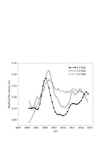
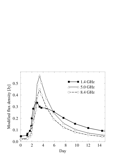
Figure 1: Observed (left) and simulated (right) lightcurves of a short–timescale flare in 0235+164. In the observed lightcurves, underlying emission has been subtracted. The model lightcurves reproduce the observed timelags, and represent only the first of the two events (J.D. 8901–8907) seen in the observed light curves.

5.2 3C 345

We have studied (Lobanov & Zensus 1999) spectral changes in the core and several jet components in 3C 345, based on the data from a VLBI monitoring of the source. In the example shown in figure 2, we use the observed trajectory (left panel of fig. 2) of the jet component C5 to confront a fit by the shock model to the variations of $S_{\rm m}$ and $\nu_{\rm m}$ (right panel of fig. 2). In the right panel, the solid line shows a fit by the shock model, without taking into account the observed kinematics of C5. When we require the shock model to reproduce $b(t)$ needed to satisfy the observed path of C5, the fit becomes problematic, at later stages of the shock evolution. This indicates that, at distances $>1$ mas, the shock may have dissipated, and other processes become main contributors to the emission from C5. Incidentally, the kinematic and emission properties of other jet features also show evidence for a change in the emission properties, at distances of 1–1.5 mas from the VLBI core of 3C 345 (Lobanov & Zensus).

Figure 2: Kinematic and spectral evolution of an enhanced emission region C5 in the jet of 3C 345. Left panel shows the observed path of C5 in the plane of the sky; right panel presents the evolution of the spectral turnover. Solid line in the right plane shows a fit by the shock model. Dashed line shows how the fit changes if the spectral evolution of the shock is required to comply with the observed path of C5.

References

- [1] raus, A., Quirrenbach, A., Lobanov, A. P. et al. 1999, A&A (subm.)
- [2] obanov, A. P. & Zensus, J. A. 1996, in ASP Conf. Series, v.100, Energy Transport in Radio galaxies and Quasars, eds. P.E. Hardee, J.A. Zensus, & A.H. Bridle (San Francisco: ASP), p.124
- [3] obanov, A. P. & Zensus, J. A. 1999, ApJ (subm.)
- [4] arscher, A. P. 1990, in Parsec–scale jets
- [5] arscher, A. P., Gear, M., & Travis, G. 1991,
- [6] oland, J., Teyssier, R., & Roos, N. 1994, A&A, 290, 357