A class of exact MHD models for astrophysical jets

Abstract

This paper examines a new class of exact and self-consistent MHD solutions which describe steady and axisymmetric hydromagnetic outflows from the atmosphere of a magnetized and rotating central object with possibly an orbiting accretion disk. The plasma is driven against gravity by a thermal pressure gradient, as well as by magnetic rotator and radiative forces. At the Alfvénic and fast critical points the appropriate criticality conditions are applied. The outflow starts almost radially but after the Alfvén transition and before the fast critical surface is encountered the magnetic pinching force bends the poloidal streamlines into a cylindrical jet-type shape. The terminal speed, Alfvén number, cross-sectional area of the jet, as well as its final pressure and density obtain uniform values at large distances from the source. The goal of the study is to give an analytical discussion of the two-dimensional interplay of the thermal pressure gradient, gravitational, Lorentz and inertial forces in accelerating and collimating an MHD flow. A parametric study of the model is also given, as well as a brief sketch of its applicability to a self-consistent modelling of collimated outflows from various astrophysical objects. The analysed model succeeds to give for the first time an exact and self-consistent MHD solution for jet-type outflows extending from the stellar surface to infinity where it can be superfast, in agreement with the MHD causality principle.

1 Introduction

Collimated outflows are ubiquitous in astrophysics and cosmic jets are observed in the radio, infrared, optical, UV and X-ray parts of the spectrum, from the ground and space, most recently via the Hubble Space Telescope. Classes of objects in association with which jets are observed include young stellar objects (Ray 1996), old mass losing stars and planetary nebulae (Livio 1997), black hole X-ray transients (Mirabel & Rodriguez 1996), supersoft X-ray sources (Kahabka & Trumper (1996), high-mass X-ray binaries, cataclysmic variables (Shahbaz et al 1997) and many AGN and quasars (Biretta 1996, Ferrari et al 1996). Despite their observed abundance however, several key questions on their acceleration and collimation among others, have not been resolved yet.

The theoretical MHD modelling of jets is not a simple undertaking, basically due to the fact that the set of the MHD equations is highly nonlinear with singular or critical points appearing in their domain of solutions; these singularities - through which a physical solution inevitably will have to pass - are not known a priori but they are determined only simultaneously with the complete solution. The purpose of the present study is to construct systematically a self-consistent MHD model for astrophysical jets from the stellar base to infinity where the interplay of the various forces acting on the plasma and which are able to accelerate and collimate the outflow, are analytically examined. This modelling is an improvement over the very few existing models developed so far to the same goal. For example, it is fully 2-dimensional (cf. Parker 1958, Weber & Davis 1967), it does not contain singularities along the symmetry axis and the outflow is not overfocused but extends to large distances (as e.g. in Blandford & Payne 1982, Ostriker 1997), the equation of state is not constrained by the artificial polytropic assumption (as e.g. in Contopoulos & Lovelace 1994, Heyvaerts & Norman 1989), the thermal pressure is meridionally anisotropic (cf. Sauty & Tsinganos 1994), the shape of the jet is self-consistently determined and not a priori given (as e.g. in Cao & Spruit 1994, Kudoh & Shibata 1997, Trussoni et al 1997), there is a steady asymptotic state (cf. Uchida & Shibata 1985, Ouyed & Pudritz 1997a,b, Goodson et al 1997), etc. Furthermore, a gap the present model aspires to fill in the existing literature is the availability of a self consistent MHD model for jet-type outflows wherein the jet speed is superfast at large distances from the base such that all perturbations are convected downstream to infinity and they do not destroy the steady state solution.

In the following Sec. 2 the basic steps for a systematic construction of this class of models are outlined. Then in Sec. 3 we discuss the critical surfaces which determine a physically interesting solution and in Sec. 4 the asymptotic behaviour of such solutions. A detailed parametric study of the model, including the solution topologies, is given in Sec. 5 and in the last Sec. 6 the connection of the dimensionless parameters characterizing the present model to the observable physical quantities of collimated outflows is briefly sketched.

2 Construction of the model

In this section we describe in some detail how our model can be systematically obtained from the closed set of the governing MHD equations.

2.1 Governing equations

The kinematics of astrophysical outflows may be described to zeroth order by the well known set of the steady ($\partial/\partial t=0$) ideal hydromagnetic equations:

$$\rho\left(\vec{V}\cdot\vec{\nabla}\right)\vec{V}=\frac{\left(\vec{\nabla}\times\vec{B}\right)\times\vec{B}}{4\pi}-\vec{\nabla}P-\rho\vec{\nabla}{\cal V}+\vec{F}_{rad}\,,$$ (1)

$$\vec{\nabla}\cdot\vec{B}=0\,,\quad\vec{\nabla}\cdot\left(\rho\vec{V}\right)=0\,,\quad\vec{\nabla}\times\left(\vec{V}\times\vec{B}\right)=0\,,$$ (2)

where $\vec{B}$, $\vec{V}$, $-\vec{\nabla}{\cal V}=-\vec{\nabla}\left(-{{\cal GM}}/{r}\right)$ denote the magnetic, velocity and external gravity fields, respectively, $\vec{F}_{rad}$ the volumetric force of radiation while $\rho$ and $P$ the gas density and pressure.
The energetics of the outflow on the other hand is governed by the first law of thermodynamics :

$$q=\rho\vec{V}\cdot\left[\vec{\nabla}\left(\frac{1}{\Gamma-1}\frac{P}{\rho}\right)+P\vec{\nabla}\frac{1}{\rho}\right]\,,$$ (3)

where $q$ is the volumetric rate of net energy input/output (Low & Tsinganos 1986), while $\Gamma=c_{p}/c_{v}$ with $c_{p}$ and $c_{v}$ the specific heats for an ideal gas.
With axisymmetry in spherical coordinates $(r,\theta,\phi)$, the azimuthal angle $\phi$ is ignorable ($\partial/\partial\phi=0$) and we may introduce the poloidal magnetic flux function $A(r,\theta)$, such that three free integrals of $A$ exist. They are the total specific angular momentum carried by the flow and magnetic field, $L(A)$, the corotation angular velocity of each streamline at the base of the flow, $\Omega(A)$ and the ratio of the mass and magnetic fluxes, $\Psi_{A}(A)$ (Tsinganos 1982). Then, the system of Eqs. (1) - (2) reduces to a set of two partial and nonlinear differential equations, i.e., the r- and $\theta$- components of the momentum equation on the poloidal plane. Note that by using the projection of the momentum equation along a stream-field line $A=const$ on the poloidal plane $(r,\theta)$, Eq. (3) becomes,

$$\rho\vec{V}\cdot\vec{\nabla}\left(\frac{1}{2}V^{2}+\frac{\Gamma}{\Gamma-1}\frac{P}{\rho}+{\cal V}-\frac{\Omega r\sin\theta}{\Psi_{A}}B_{\phi}\right)-\vec{V}\cdot\vec{F}_{rad}=q\,.$$ (4)

For a given set of the integrals $L(A)$, $\Omega(A)$ and $\Psi(A)$, equations (1) - (2) - (3) could be solved to give $\rho(r,\theta)$, $P(r,\theta)$ and $A(r,\theta)$, if the heating function $q(r,\theta)$ and the radiation force $\vec{F}_{rad}$ are known. Similarly, one may close this system of Eqs. (1) - (2) - (3), if an extra functional relation of $q$ with the unknowns $\rho$, $P$ and $A$ exists. As an example, consider the following special functional relation of $q$ with the unknowns $\rho$, $P$ and $A$ (Tsinganos et al 1992),

$$q=\frac{\gamma-\Gamma}{\Gamma-1}\frac{P}{\rho}\vec{V}\cdot\vec{\nabla}\rho\,,$$ (5)

where $\gamma\leq\Gamma$. Then, Eq. (3) can be integrated at once to give the familiar polytropic relation between $P$ and $\rho$,

$$P=Q\left(A\right)\rho^{\gamma}\,,$$ (6)

for some function $Q(A)$ corresponding to the enthalpy along a poloidal surface $A=const$. In this special case we can integrate the projection of the momentum equation along a stream-field line $A=const$ on the poloidal plane, Eq. (4) by further assuming that $\vec{V}\cdot\vec{F}_{rad}=0$, to get the well known Bernoulli integral which subsequently can be combined with the component of the momentum equation across the poloidal fieldlines (the transfield equation) to yield $\rho$ and $A$. After finding a solution, one may go back to Eq. (3) and fully determine the function $q(r,\theta)$. It is evident that even in this special polytropic case with $\gamma\neq\Gamma$ the heating function $q$ (not its functional form but the function $q(r,\theta)$ itself) can be found only a posteriori. Note that for $\gamma=\Gamma$ and only then the flow is isentropic.
Evidently, it is not possible to integrate Eq. (3) for any functional form of the heating function $q$, such as it was possible with the special form of the heating function given in Eq. (5). To proceed further then and find other more general solutions (effectively having a variable value for $\gamma$), one may choose some other functional form for the heating function $q$ and from energy conservation, Eq. (3), derive a functional form for the pressure. Equivalently, one may choose a functional form for the pressure $P$ and determine the volumetric rate of thermal energy a posteriori from Eq. (3), after finding the expressions of $\rho$, $P$ and $A$ which satisfy the two remaining components of the momentum equation. Hence, in such a treatment the heating sources which produce some specific solution are not known a priori; instead, they can be determined only a posteriori. However, it is worth to keep in mind that as explained before, this situation is analoguous to the more familiar constant $\gamma$ polytropic case, with $\gamma\neq\Gamma$. In this paper we shall follow this approach, which is further illustrated in the following section.

However, even with this approach, the integration of the system of mixed elliptic/hyperbolic partial differential equations (1) - (2) is not a trivial undertaking. Besides its nonlinearity, this is largely due to the fact that a physically interesting solution is bound to cross some critical surfaces which are not known a priori but they are determined simultaneously with the solution. For this reason only a very few such self-consistent solutions are available, albeit no one is superfast at infinity. Further assumptions on the shape of the critical surfaces are needed, as discussed in the following.

2.2 Assumptions

In order to construct analytically a new class of exact solutions, we shall proceed by making the following two key assumptions:

1. that the Alfvén number $M$ is some function of the dimensionless radial distance $R={r/r_{\star}}$, i.e., $M=M(R)$
   and

2. that the poloidal velocity and magnetic fields have a dipolar angular dependence,

   $$A={r_{\star}^{2}B_{\star}\over 2}{\cal A}\left(\alpha\right)\,,\qquad\alpha=\frac{R^{2}}{G^{2}\left(R\right)}\sin^{2}\theta\,,$$ (7)

for some function $G(R)$.

A few words on the physical basis of the above two assumptions are needed at this point. These assumptions are expected to be physically reasonable for describing the outflow properties close to the rotation and magnetic axis of the system. There, far from the distortion caused by the presence of an accretion disk, the angular distribution of the stellar magnetic field may be approximately dipolar (see Fig. 1 in Ghosh & Lamb 1979). On the other hand, regarding the assumption of spherical critical surfaces, we note that all available numerical models derive a shape of the Alfvén surface which is approximately spherical near the rotation and magnetic axis of the system (Sakurai 1985, Bogovalov & Tsinganos 1999, Ustyugova et al 1999). Hence, although the analysed model may in principle extend to all angles from the symmetry axis since it satisfies the governing MHD equations, its physical applicability could be constrained around the polar regions only.

We are interested in transAlfvenic flows and denote by a $\star$ the respective value of all quantities at the Alfvén surface. By choosing the function $G(R)$ such that $G\left(R=1\right)=1$ at the Alfvén transition $R=1$, it is evident that $G(R)$ measures the cylindrical distance $\varpi$ to the polar axis of each fieldline labeled by $\alpha$, normalized to its cylindrical distance $\varpi_{\alpha}$ at the Alfvén point, $G\left(R\right)={\varpi}/{\varpi_{\alpha}}$. For a smooth crossing of the Alfvén sphere $R=1$ [$r=r_{\star},\theta=\theta_{a}(\alpha)$], the free integrals $L$ and $\Omega$ are related by

$${L\over\Omega}=\varpi_{\alpha}^{2}(A)=r_{\star}^{2}\sin^{2}\theta_{a}(\alpha)=r_{\star}^{2}\alpha\,.$$ (8)

Therefore, the second assumption is equivalent with the statement that at the Alfvén surface the cylindrical distance $\varpi_{\alpha}$ of each magnetic flux surface $\alpha=const$ is simply proportional to $\sqrt{\alpha}$.
Instead of using the three remaining free functions of $\alpha$, (${\cal A}\,,\Psi_{A}$ , $\Omega$), we found it more convenient to work instead with the three dimensionless functions of $\alpha$, ($g_{1}$ , $g_{2}$ , $g_{3}$),

$$g_{1}\left(\alpha\right)=\int{\cal A}^{{}^{\prime}2}d\alpha\,,$$ (9)

$$g_{2}\left(\alpha\right)=\frac{r_{\star}^{2}}{B_{\star}^{2}}\int\Omega^{2}\Psi_{A}^{2}d\alpha$$ (10)

$$g_{3}\left(\alpha\right)=\frac{\Psi_{A}^{2}}{4\pi\rho_{\star}}\,.$$ (11)

These functions $g_{1}(\alpha),\,g_{2}(\alpha),\,g_{3}(\alpha)$ are vectors in a 3D $\alpha$-space with some basis vectors $u_{1}(\alpha)$, $u_{2}(\alpha)$, $u_{3}(\alpha)$ (Vlahakis & Tsinganos (1998), hereafter VT98). Note that the forms of $g_{1}\,,g_{2}\,,g_{3}$ or equivalently the forms of $A$, $\Psi_{A}$, $\Omega$, $L=r_{\star}^{2}\alpha\Omega$ and $P$ should be such that the two remaining components of the momentum equation are separable in the $\alpha$ and $R$ coordinates.

2.3 The method

The main steps of the general method for getting exact solutions under the previous two assumptions are briefly the following.

First, by using $\alpha$ instead of $\theta$ as the independent variable, we transform from the pair of the independent variables ($R\,,\theta$) to the pair of the independent variables ($R\,,\alpha$). The resulting form of the $\alpha$- component of the momentum equation can be integrated at once to yield for the gas pressure,

$$P(R,\alpha) = \frac{B_{\star}^{2}}{8\pi}\left(f_{0}+f_{4}g_{1}+f_{1}g_{1}^{{}^{\prime}}+f_{2}\alpha g_{1}^{{}^{\prime}}+f_{5}g_{2}+f_{3}\alpha g_{2}^{{}^{\prime}}\right)$$ (12)

$$= \frac{B_{\star}^{2}}{8\pi}{\bf{Y}}{\bf{P}}^{{\dagger}}\,,$$

where $f_{0}\left(R\right)$ is a free function emerging from this integration, $f_{i}\left(R\right)$, $i=1,2,\dots,$ are functions of the spherical radius $R$ given in the Appendix A and P and Y are the (1 $\times$ 7) matrices,

$${\bf{Y}}=\left[\;1\,\;g_{1}\,\;g_{1}^{{}^{\prime}}\,\;\alpha g_{1}^{{}^{\prime}}\,\;g_{2}\,\;\alpha g_{2}^{{}^{\prime}}\,\;g_{3}\,\right]\,,$$ (13)

$${\bf{P}}=\left[\;f_{0}\,\;f_{4}\,\;f_{1}\,\;f_{2}\,\;f_{5}\,\;f_{3}\,\;0\,\right]\,.$$ (14)

Second, by substituting Eq. (12) in the r-component of the momentum equation we obtain in terms of the (1 $\times$ 7) matrix X

$${\bf{X}}=\left[\;f_{0}^{{}^{\prime}}\,\;f_{4}^{{}^{\prime}}\,\;-\!f_{6}\,\;-\!f_{7}\,\;f_{5}^{{}^{\prime}}\,\;-\!f_{8}\,\;-\!f_{9}\;\right]\,,$$ (15)

the following equation:

$${\bf{Y}}{\bf{X}}^{{\dagger}}={\bf{0}}\,.$$ (16)

A key step in the method is to find a possible set of vectors $u_{1}(\alpha)$, $u_{2}(\alpha)$, $u_{3}(\alpha)$ such that all components of the matrix Y belong to the same $\alpha$-space. To that goal we choose $u_{1}(\alpha)=1$ and $u_{2}(\alpha)=g_{1}(\alpha)$. If this is the case, then our third step is to construct a $3\times 7$ matrix ${\bf{K}}$ such that

$${\bf{Y}}=\left[\;{u_{1}}\,\;{u_{2}}\,\;{u_{3}}\;\right]{\bf{K}}\,.$$ (17)

Then, from Eq. (16),

$$\left[\;{u_{1}}\,\;{u_{2}}\,\;{u_{3}}\;\right]\,{\bf{K}}{\bf{X}}^{{\dagger}}={\bf{0}}\,,$$

and since ${u_{i}}$ are linearly independent it follows

$${\bf{K}}{\bf{X}}^{{\dagger}}={\bf{0}}\,.$$ (18)

Finally, it follows from Eq. (12) , (14) and (17) that,

$$P=\frac{B_{\star}^{2}}{8\pi}\left(P_{0}+g_{1}P_{1}+u_{3}P_{2}\right)\,,$$

where the three components of the pressure $P_{0}$, $P_{1}$ and $P_{2}$ are

$$[P_{0}\;P_{1}\;P_{2}]^{{\dagger}}={\bf K}{\bf P}^{{\dagger}}\,.$$ (19)

2.4 The Model

Let us know apply this method in the construction of a specific model. We may recall that in a previous paper, (VT98), it was found that only nine distinct general families of such vectors exist. One of them is,

$$u_{1}(\alpha)=1\,,\quad u_{2}(\alpha)=\alpha\,,\quad u_{3}(\alpha)=\alpha^{\epsilon}\,,$$ (20)

while the corresponding free functions are,

$$g_{1}(\alpha)=a\,,$$ (21)

$$g_{2}(\alpha)=\xi\alpha+{\mu\alpha^{\epsilon}/\epsilon}\,,$$ (22)

$$g_{3}(\alpha)=1+\delta\alpha+\mu\delta_{0}\alpha^{\epsilon}\,.$$ (23)

For these particular choice of $u_{1}(\alpha)=1\,,u_{2}(\alpha)=\alpha\,,u_{3}(\alpha)=\alpha^{\epsilon}$ we find the following form of the matrix K,

$${\bf{K}}=\left[\begin{array}[]{ccccccc}1&0&1&0&0&0&1\\ 0&1&0&1&\xi&\xi&\delta\\ 0&0&0&0&\displaystyle\frac{\mu}{\epsilon}&\mu&\mu\delta_{0}\end{array}\right]\,.$$ (24)

Then, from Eqs. (14) and (19) we get,

$$\left[\begin{array}[]{c}P_{0}\\ P_{1}\\ P_{2}\end{array}\right]=\left[\begin{array}[]{l}f_{0}+f_{1}\\ f_{4}+f_{2}+\xi\left(f_{3}+f_{5}\right)\\ \mu\left(\displaystyle\frac{f_{5}}{\epsilon}+f_{3}\right)\end{array}\right]\,.$$ (25)

Finally, from Eq. (18) using the definitions of Eqs. (15), (24) we obtain, three ordinary differential equations, the system (51), for the functions of $R$ in the model for $\epsilon\neq 0,1$ and $\mu\neq 0$ (only then we have a 3D $\alpha$-space with $1\,,\alpha\,,\alpha^{\epsilon}$ linearly independent).

Figure 1: An illustration of the construction of the streamlines $\alpha=const.$ on the poloidal plane in meridionally selfsimilar outflows.

Altogether, let us summarize the characteristics of our model. The physical quantities of the outflow have the following exact expressions:

$$\rho=\frac{\rho_{\star}}{M^{2}}\left(1+\delta\alpha+\mu\delta_{0}\alpha^{\epsilon}\right)$$ (26)

$$P=\frac{\rho_{\star}V_{\star}^{2}}{2}\left(P_{0}+P_{1}\alpha+P_{2}\alpha^{\epsilon}\right),$$ (27)

$$\vec{V}=V_{\star}\left(\frac{M^{2}\cos{\theta}}{G^{2}}\hat{r}-\frac{M^{2}F\sin{\theta}}{2G^{2}}\hat{\theta}+\right.$$

$$\left.\sqrt{\xi\alpha+\mu\alpha^{\epsilon}}\frac{G^{2}-M^{2}}{G\left(1-M^{2}\right)}\hat{\phi}\right)/\sqrt{1+\delta\alpha+\mu\delta_{0}\alpha^{\epsilon}}$$ (28)

$$\vec{B}=B_{\star}\left(\frac{\cos{\theta}}{G^{2}}\hat{r}-\frac{F\sin{\theta}}{2G^{2}}\hat{\theta}-\right.$$

$$\left.\sqrt{\xi\alpha+\mu\alpha^{\epsilon}}\frac{1-G^{2}}{G\left(1-M^{2}\right)}\hat{\phi}\right)\,,$$ (29)

where the five unknown functions $G^{2}(R)$, $F(R)$, $M^{2}(R)$, $P_{1}(R)$ and $P_{0}(R)$ entering in the above expressions are obtained from the integration of the five first order ordinary differential equations given in Appendix B, while the pressure component $P_{2}(R)$ is given explicitly in terms of the other variables (Appendix B).

Note that the parameters $\epsilon$ and $\xi$ determine the enclosed poloidal current by a given magnetic surface in the outflow. The parameters $\epsilon\,,\delta\,,\delta_{0}$ determine the latitutianal distribution of the density. The parameter $\mu$ controls the differential rotation. Further discussion of the physical meaning of these parameters will be given later (Secs. 2.5, 5).

2.5 Some properties of the meridionally self-similar model

Our model is meridionally self-similar, i.e., if we know the shape of one fieldline $\alpha=\alpha_{1}$ we may derive the shape of any other streamline $\alpha=\alpha_{2}$ by moving in the meridional direction along each cycle $R=const$ on the poloidal plane as illustrated in Fig. (1).

Note that the flux function $A$ is simply proportional to $\alpha$ which means that for cylindrical solutions at $R\gg 1$, the magnetic field on the poloidal plane is uniform and its strength is independent of $\alpha$, $\mid\vec{B_{p}}\mid_{\infty}={B_{\star}}/{G_{\infty}^{2}}$.

The density at the Alfvén surface is

$$\rho_{\alpha}=\frac{\Psi_{A}^{2}}{4\pi}=\rho_{\star}\left(1+\delta\alpha+\mu\delta_{0}\alpha^{\epsilon}\right)\,,$$

i.e., it is similar to a Taylor expansion in the cylindrical distance $\varpi_{\alpha}$ from the rotation and magnetic axis $\alpha=0$. For example, for $\epsilon=0.5$ we have,

$$\frac{\rho_{\alpha}}{\rho_{\star}}=1+\mu\delta_{0}\frac{\varpi_{\alpha}}{r_{\star}}+\delta\left(\frac{\varpi_{\alpha}}{r_{\star}}\right)^{2}\,.$$

We ’ve also introduced the expansion factor

$$F\equiv\frac{\partial\ln\alpha(R,\theta)}{\partial\ln R}=2-R\frac{G^{2^{\prime}}}{G^{2}}\,,$$

which measures the opening of the fieldlines on the poloidal plane, as illustrated in Fig. (2).

Figure 2: A geometrical illustration of the expasion factor $F(R)$ which determines the shape of the poloidal streamlines in a meridionally selfsimilar outflow.

Thus, if $F>2$ the fieldlines turn towards the axis, if $F=2$ they expand cylindrically, if $F=0$ they are purely radial while if $F<0$ the fieldlines turn toward the equator (in that case, there is a closed region near the equator). If we eliminate $F$ in Eq. (58) (using Eq. (52) ) we have the second derivative of $G$ (which corresponds to the term $\frac{\partial^{2}A}{\partial r^{2}}$ of the transfield equation). So, using $F$ us an intermediate function we have only first order differential equations.

2.6 Radiative acceleration

For the radiative acceleration we have assumed two components. The first component is due to continuum absorption and is set proportional to the radiative flux. It drops with distance as $r^{-2}$, similarly to gravity. If $L_{\varepsilon}$ is the Eddington luminocity, we may use the ratio $\Gamma_{\varepsilon}={L}/{L_{\varepsilon}}$ such that this part of the radiative acceleration is $\Gamma_{\varepsilon}\rho{{\cal GM}}/{r^{2}}$.
We have also assumed a second component of the radiative acceleration due to line contribution. By adopting the optically thin atmosphere aproximation (Lamers, 1986, Chen & Marlborough 1994, Kakouris & Moussas 1997), this part of the acceleration is simply a function of $r$ since in general the total number of weak lines is a function of $r$. Then, the corresponding expression of the radiative acceleration is ${V_{\star}^{2}}/{r_{\star}}\rho Q\left(R\right)$.

The combination of gravitational and radiative acceleration is thus

$$-\rho\vec{\nabla}{\cal V}+\vec{F}_{rad}=\frac{V_{\star}^{2}}{r_{\star}}\rho\left(Q\left(R\right)-\frac{\nu^{2}}{2R^{2}}\right)\hat{r}\,,$$

where

$$\nu^{2}=\frac{V_{esc}^{2}}{V_{\star}^{2}}\left(1-\Gamma_{\varepsilon}\right)=\frac{2{\cal GM}}{r_{\star}V_{\star}^{2}}\left(1-\Gamma_{\varepsilon}\right)\,.$$

Furthermore, we use for $Q$ the aproximation of a power law, $Q\left(R\right)={\mu_{0}}/{R^{x}}$ with $\mu_{0}$, and $x$ constants.

In the following we shall discuss the results of the integration. Finally, we shall calculate all the other remaining physical quantities. A parametric study will be made only for $\epsilon>0$, since for $\epsilon<0$ we have $\rho\rightarrow\infty$ as $\alpha\rightarrow 0$.

For $\epsilon=0$ or $1$ (or equivalently for $\mu=0$), we get a degenerate case which needs an extra condition between the functions of $R$. This case has been studied in Sauty & Tsinganos (1994) (where the components of the pressure $P_{0}\,,P_{1}$ are set proportional to each other) and Trussoni et al (1997) (where the function $G(R)$ is given a priori). Here, in the case $\mu=0$ we ’ve chosen this extra condition to be ${f_{5}^{{}^{\prime}}}/{\epsilon}-f_{8}-\delta_{0}f_{9}=0$ (c.f., the last equation of the system (51).

3 Critical Surfaces

In the domain of the solutions there exist several critical surfaces. In the following we briefly discuss the physical context of these critical surfaces.

3.1 Alfvén critical surface

We recall that one of our goals is to investigate transalvfenic solutions wherein $L=\varpi_{\alpha}^{2}\Omega$. By multiplying Eq. (58) with $1-M^{2}$ and evaluating the resulting expression at the Alfvén point we get

$$F_{\star}p_{\star}-\frac{F_{\star}^{2}-4}{2}-2P_{1\star}=0\,,$$ (30)

with $F_{\star}$, $P_{1\star}$ and $p_{\star}=\displaystyle{\left({dM^{2}}/{dR}\right)_{\star}}$ the respective values of these quantities at the Alfvén transition $R=1$. Eq. (30) is the so-called Alfvén regularity condition in the present model. Note that if we also multiply Eq. (68) with $1-M^{2}$ and evaluate the resulting expression at the Alfvén point we get an identical expression while Eq. (62) after using L’Hospital’s rule gives an identity.

3.2 Slow/fast critical surfaces.

In order to locate the critical surfaces where the radial component of the flow speed equals to the corresponding slow/fast MHD wave speeds (Tsinganos et al 1996), we need to calculate first the sound speed $C_{s}$ at these points; to this goal we may proceed as follows.
Consider that at some fixed distance $R$ of a given streamline labeled by $\alpha$ we make a small change in the density $\rho$ and the pressure $P$. We may define the square of the sound speed as the ratio of such an infinitesimal change of $P$ and $\rho$,

$$\displaystyle{C_{s}^{2}=\left(\frac{\partial P}{\partial\rho}\right)_{\alpha,R}=-\frac{V_{\star}^{2}}{2}\frac{M^{4}}{\displaystyle{1+\delta\alpha+\mu\delta_{0}\alpha^{\epsilon}}}}\times$$

$$\displaystyle{\left(\frac{\partial P_{0}\left(R,M^{2}\right)}{\partial M^{2}}+\frac{\partial P_{1}\left(R,M^{2}\right)}{\partial M^{2}}\alpha+\frac{\partial P_{2}\left(R,M^{2}\right)}{\partial M^{2}}\alpha^{\epsilon}\right)}\,,$$ (31)

using Eqs. (26) - (27). But from the differential equation (70) we can calculate the derivative ${\partial P_{0}\left(R,M^{2}\right)}/{\partial M^{2}}$ while from Eq. (68) after substituting $dF/dR$ from Eq. (58) we can calculate the other derivative ${\partial P_{1}\left(R,M^{2}\right)}/{\partial M^{2}}$. Finally, from Eq. (71) by taking the derivative of $P_{2}(G,M^{2})$ for constant $G(R)$ we get similarly the derivative ${\partial P_{2}\left(R,M^{2}\right)}/{\partial M^{2}}$. Substituting these derivatives in Eq. (3.2) we obtain the expression of the sound speed at the points where $\left(2M^{2}-1\right)G^{4}-M^{4}=0$.
An inspection of Eq. (62) for the Alfvén number $M(R)$ reveals that besides the Alfvén transition where $M=G=R=1$, there may be other distances $R_{x}\neq 1$ where the denominator of this equation becomes zero, ${\cal D}\equiv\left[\left(2M^{2}-1\right)G^{4}-M^{4}\right]_{R=R_{x}}=0$. In such a case, the numerator of Eq. (62) should be also set equal to zero and we have conditions typical of a critical point (using L’Hospital’s rule we find two solutions for the slope of $M^{2}$ in this point, i.e., this singularity corresponds to an x-type critical point). To clarify the physical identity of such a critical point, we may manipulate the denominator ${\cal D}$ and write it in the form

$$\displaystyle{{\cal D}=2\epsilon G^{2}\frac{1+\delta\alpha+\mu\delta_{0}\alpha^{\epsilon}}{V_{\star}^{2}V_{A,r}^{4}\mu\alpha^{\epsilon}}}\times$$

$$\displaystyle{\left(V_{r}^{2}-V_{A,r}^{2}\right)\left[V_{r}^{4}-V_{r}^{2}\left(C_{s}^{2}+V^{2}_{A}\right)+C_{s}^{2}V^{2}_{A,r}\right]}\,,$$ (32)

where $V_{A}$, $V_{A,r}$ are the total and radial Alfvén speeds, respectively. Evidently, a critical point at $R_{x}$ corresponds to the modified by the meridional self-similarity fast/slow critical points (Tsinganos et al 1996). In other words, the sphere $R=R_{x}$ is the corresponding spherical separatrix in the hyperbolic domain of the system of the MHD differential equations (Bogovalov 1996). The sound speed is well defined at the critical points where ${\cal D}=0$, but it is an open question if this definition can be extended everywhere.

4 Asymptotic analysis

According to the asymptotical behaviour of the poloidal streamlines we may distinguish two different types of solutions.

4.1 Cylindrical asymptotics achieved through oscillations (Type I solutions)

In this case the poloidal streamlines undergo oscillations of decaying amplitude and finally they become cylindrical. A similar oscillatory behaviour is found in all physical quantities, a situation which has been already analysed in detail (Vlahakis & Tsinganos, 1997, henceforth VT97). According to this analysis, as $R\gg 1$ we have

$$M^{2}=M_{\infty}^{2}\left(1+\lambda_{0}\varepsilon\right)\,,\quad G^{2}=G_{\infty}^{2}\left(1-\varepsilon\right)\,,$$ (33)

$$\varepsilon(r)\approx\frac{D}{r^{s}}\sin{\left(kr+\phi_{0}\right)}\,,\quad s=2+\frac{\lambda_{0}M_{\infty}^{2}}{M_{\infty}^{2}-1}\,,$$ (34)

$$k^{2}=\frac{2\xi\left(1-\epsilon\right)\left(M_{\infty}^{2}-G_{\infty}^{4}\right)}{r_{\star}^{2}M_{\infty}^{2}\left(1-M_{\infty}^{2}\right)^{2}}\,,$$ (35)

$$\lambda_{0}=\left[\left(\epsilon+1\right)M_{\infty}^{2}-\left(\epsilon-1\right)G_{\infty}^{4}\right]\frac{1-M_{\infty}^{2}}{\left(2M_{\infty}^{2}-1\right)G_{\infty}^{4}-M_{\infty}^{4}}\,.$$ (36)

Note that for $s>1$ the gravitational term is dominant, but the analysis is still correct because the oscillatory perturbation is independent of the ”backround” term $1/r$ (VT97).

4.2 Converging to the axis asymptotics (Type II solutions)

An analysis of the system of the differential equations (58) - (70) for $G(R\rightarrow\infty)\rightarrow 0$, $M(R\rightarrow\infty)\rightarrow\infty$ and $F(R\rightarrow\infty)\rightarrow F_{\infty}$ shows that in this case the value of the expansion factor $F_{\infty}$ at $R\gg 1$ approaches a constant value, the positive root of the equation

$$\left(\epsilon+3\right)\left(\epsilon+\frac{3}{2}\right)F_{\infty}^{2}-2\left(\epsilon+2\right)\left(\epsilon+\frac{5}{2}\right)F_{\infty}-4\left(\epsilon+2\right)=0\,.$$

As we shall see later, solutions are obtained mainly for $\epsilon>0$, in which case this root is greater than 2, $F_{\infty}>2$, i.e., the cross-sectional area of flow tube drops to zero at large radii, $G^{2}\propto R^{2-F_{\infty}}$. The poloidal velocity goes to infinity as $V_{r}\propto R^{\left(\epsilon+2\right)\left(F_{\infty}-2\right)}$ to conserve mass, while the toroidal velocity grows like $V_{\phi}(R\rightarrow\infty)\propto R^{F_{\infty}-2}$ from angular momentum conservation.

5 Parametric study of solutions

The two crucial parameters which affect the qualitative behaviour of the model are $\xi$ and $\epsilon$.
First for $\epsilon$, from the expression of the density $\rho$ in Eq. (26) it is required that $\epsilon>0$ in order that the density at the axis, $\rho(\alpha=0,R)$ and the pressure are finite. In the case $\epsilon=1$ the electric current $I_{z}(\alpha,R)$ enclosed by a poloidal magnetic flux tube $\alpha=const.$ and the corresponding confining azimuthal magnetic field $B_{\phi}(\alpha,R)$ are proportional to $\alpha$; this case has been already studied in Sauty & Tsinganos (1994) and it was found that cylindrical asymptotics is obtained through oscillations. If $\epsilon>1$, $I_{z}(\alpha,R)$ and $B_{\phi}(\alpha,R)$ are increasing faster with $\alpha$ which results in a stronger magnetic pinching force which eventually reduces the cross-sectional area of the flow tube to zero. Therefore we expect that when $0<\epsilon<1$ we obtain asymptotically cylindrical solutions while for larger values solutions where asymptotically $G_{\infty}\longrightarrow 0$, as it may be seen in Figure (11). For the larger values of $\epsilon>1$ the pinching is so strong that oscillations do not exist. This may also be seen from Eq. (35) where $k^{2}<0$ for $\epsilon>1$ (for $\xi(M^{2}_{\infty}-G_{\infty}^{4})>0$). Note that if $\epsilon>1$, it is needed to have $\xi>0$ such that the square roots in Eqs. (49), (50) are positively defined near the axis $\alpha\approx 0$.

Altogether then, we shall divide accordingly our parametric study to the intervals $0<\epsilon<1$, for cylindrical asymptotics with oscillations [cases (a)-(b)] and $\epsilon>1$, for converging to the axis fieldlines without oscillations [case (c)] .
Second, the parameter $\xi$ is related to the asymptotic value of the pressure component $P_{1}$ (and through force balance in the cylindrical direction to $B_{\phi}$ and $I_{z}$). For cylindrical solutions at $R\gg 1$ we get from the asymptotic analysis

$$P_{1,\infty}=-\xi\left(\frac{\left(M^{2}-1\right)\left(G^{4}-M^{2}\right)+M^{2}\left(1-G^{2}\right)^{2}}{G^{2}M^{2}\left(1-M^{2}\right)^{2}}\right)_{\infty}\,.$$

For example when $\xi>0$, in which case from the integration we find $G_{\infty}<1\ll M_{\infty}$, we obtain $P_{1,\infty}>0$ and the pressure gradient assists the magnetic pressure in collimating the outflow. In that respect solutions with $\xi>0$ correspond to an underpressured jet (Trussoni et al 1997). On the other hand when $\xi<0$ in which case from the integration $G_{\infty}^{4}>M^{2}_{\infty}>1$ and we find $P_{1,\infty}>0$, $P_{2,\infty}<0$. In all solutions with cylindrical asymptotics (i.e., for $\epsilon<1$), one finds that for $\xi>0$ the total pressure force in the $\hat{\varpi}$ direction $-\hat{\varpi}\vec{\nabla}\left(P+\frac{B^{2}}{8\pi}\right)$ is towards the axis while for $\xi<0$ it is in the opposite direction.

Figure 3: Poloidal streamlines close and far from the central object for case (a) with parameters: $\epsilon=0.5$, $\xi=10$, $\delta\nu^{2}=3.5$, $\delta_{0}\nu^{2}=0.1$, $\mu_{0}=0$, $F_{\star}=1$ and $p_{\star}\approx 2.2655$. The Alfvén (fast) surface is indicated by dashed (dot-dashed) lines.

Figure 4: Dimensionless velocities for case (a) with parameters: $\epsilon=0.5$, $\xi=10$, $\delta\nu^{2}=3.5$, $\delta_{0}\nu^{2}=0.1$, $\mu_{0}=0$, $F_{\star}=1$ and $p_{\star}\approx 2.2655$

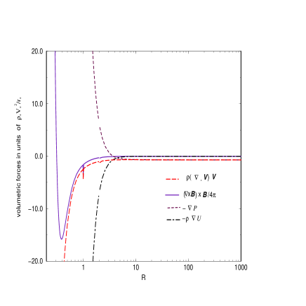
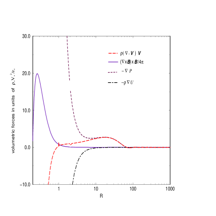
Figure 5: In the left panel are plotted the components of the magnetic (solid), pressure gradient (small dashes), gravitational (dot-dashed) and total acceleration (long dashes) perpendicular to the poloidal streamlines on line $\alpha=\alpha_{lim}$ for the parameters of the previous figure. In the the right panel the corresponding components parallel to the poloidal lines are plotted also for case (a) and the same parameters: $\epsilon=0.5$, $\xi=10$, $\delta\nu^{2}=3.5$, $\delta_{0}\nu^{2}=0.1$, $\mu_{0}=0$, $F_{\star}=1$ and $p_{\star}\approx 2.2655$

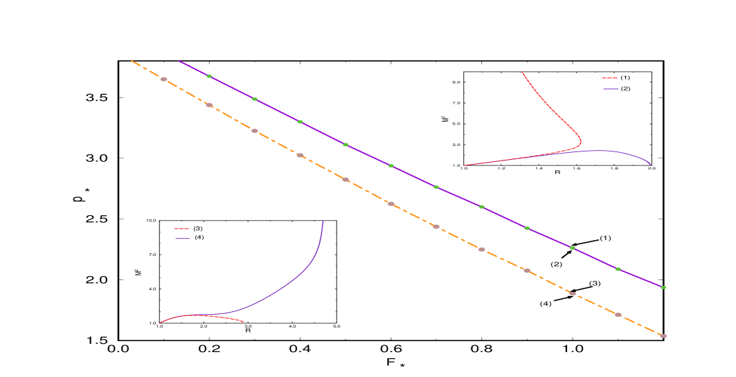
Figure 6: The solid line gives the relation between the expansion factor $F_{\star}$ and the slope $p_{\star}$ of $M^{2}(R)$ at the Alfvén point for a solution through all critical points, for case (a) with parameters: $\epsilon=0.5$, $\xi=10$, $\delta\nu^{2}=3.5$, $\delta_{0}\nu^{2}=0.1$, $\mu_{0}=0$. The topologies of $M^{2}(R)$ at the neighboring points (1), (2), (3) and (4) are also shown.

In all these cases we have $\xi(M^{2}_{\infty}-G_{\infty}^{4})>0$, or, $\xi\left(\left({\rho V_{r}^{2}}/{2}\right)_{\alpha=0,R\gg 1}-\left({\rho V_{r}^{2}}/{2}\right)_{\alpha=0,R=1}\right)>0$. In other words the sign of $\xi$ determines if the poloidal kinetic energy on the axis is larger at the Alfvén point or at infinity. Thus, according to the range of values of $\xi$ and $\epsilon$ we distinguish the following cases:

5.1 Case (a): $0<\epsilon<1$, $\xi>0$

In this case cylindrical asymptotics is achieved through small amplitude oscillations of decaying amplitude (Type I solutions). In the left panel of Fig. (3) the shape of the field/streamlines on the poloidal plane is shown in the inner region between the stellar base, the Alfvén (dashed, $R=1$) and fast (dot-dashed, $R=2$) critical surfaces. The poloidal lines are almost radial up to the Alfvén surface while after the fast critical surface they have attained a cylindrical shape. However, the final cylindrical shape of the poloidal field/stream lines is reached further out, i.e., at about $R=20$, as it is shown in the larger scale of Fig. (3) (right panel) where their asymptotically cylindrical shape can be better seen. The bending of the poloidal field/stream lines towards the magnetic/rotational axis is caused by the magnetic pinching force as it can be seen in the left panel of Fig. (5) where the various components of the forces acting on the plasma perpendicular to the poloidal fieldlines are plotted. In the inner region of the outflow, the total inertial force perpendicular to the lines (centripetal force) is almost exclusively provided by the inwards magnetic force, with the outwards pressure gradient balancing the inward component of gravity. Asymptotically however, the magnetic pinching force and gravity are neglegible and the pressure gradient of the underpressured jet balances the centrifugal force. The acceleration of the plasma along the poloidal lines can be seen in the right panel of Fig. (5). Evidently, in the inner region gravity is balanced by the pressure gradient force and the plasma is accelerated only by the remaining magnetic force while in the outer region where gravity and the magnetic force are negligible, it is accelerated by the dominant pressure gradient force. As it may also seen in Fig. (4) most of the acceleration occurs on the far region at $R\lower 2.0pt\hbox{$\buildrel{\scriptstyle>}\over{\scriptstyle\sim}$}10$ by the thermal pressure gradient force.

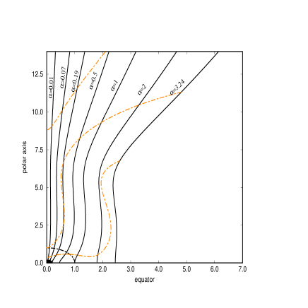
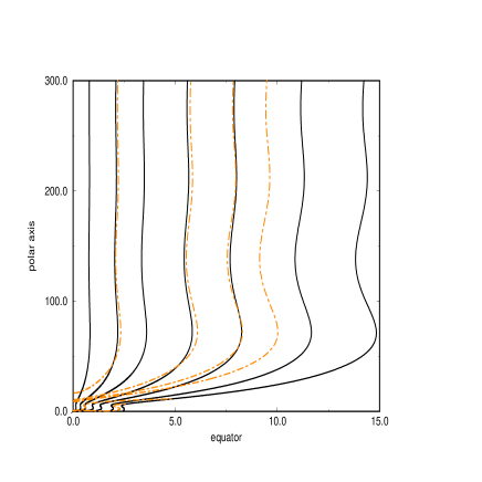
Figure 7: Poloidal streamlines close and far from the central object for case (b) with parameters: $\epsilon=0.5$, $\xi=-5$, $\delta\nu^{2}=4$, $\delta_{0}\nu^{2}=0.001$, $\mu_{0}=0$, $F_{\star}=1$ and $p_{\star}=2$. With dotted lines the density isocontoures are indicated with $\rho/\rho_{\star}=0.1,1,10$ from top to bottom in the left panel and $\rho/\rho_{\star}=0.01,0.04,0.07,1,10$ from left to right in the right panel. The Alfvén surface in the left panel is indicated by dashed lines.

Figure 8: Dimensionless velocities for case (b) with parameters: $\epsilon=0.5$, $\xi=-5$, $\delta\nu^{2}=4$, $\delta_{0}\nu^{2}=0.001$, $\mu_{0}=0$, $F_{\star}=1$ and $p_{\star}=2$

The solution discussed in this representative example crosses the modified by self-similarity fast critical point and a note is in order here on how such a solution may be obtained. First, we integrate Eqs. (58) – (70) downstream of the Alfvén critical point at which $R=G=M=1$, $F=F_{\star}$, $P_{1}=P_{1\star}$ and $P_{0}=P_{0\star}$, a free parameter which determines the pressure at infinity. At $R=1$ the Alfvén regularity condition relates $F_{\star}$, $p_{\star}$ and $P_{1\star}$, Eq. (30). Also there is a relation between $F_{\star}$,$p_{\star}$ such that the solution passes through the fast critical point; this is the solid line in Fig. (6). Assume for example that we choose $F_{\star}=1$ and we vary $p_{\star}$, Fig. (6). There is only one value of $p_{\star}\approx 2.26$ which satisfies the Alfvén regularity condition and the solution crosses the fast critical point. For other values of $p_{\star}$ above and below $p_{\star}\approx 2.26$ we have three different types of unphysical solutions shown in Fig. (6):

• from point (1) of Fig. (6) corresponding to $p_{\star}$ higher than $2.26$ we get solutions in which the denominator of the differential equation for $M^{2}$ becomes zero and the curve $M^{2}(R)$ turns back to smaller distances,

• from point (2) of Fig. (6) corresponding to $p_{\star}$ lower than $2.26$ till point (3) we get solutions in which the numerator of the differential equation for $M^{2}$ becomes zero and then the solutions become again subAlfvénic,

• finally, from point (4) of Fig. (6) we get solutions in which there is a distance $R$ wherein $M\rightarrow\infty$ and the solutions terminate there.

A fine tuning between points (1) and (2) gives the unique solution which goes to infinity with superAlfvénic and superfast radial velocity, satisfying also the causality principle for the propagation of MHD perturbations. After finding such a critical value for $p_{\star}$ we also integrate Eqs. (58) - (70) upstream of the Alfvén point.

5.2 Case (b): $0<\epsilon<1$, $\xi<0$

In this case we may have two possibilities. In one the solution crosses the fast critical point and the situation is similar to the previous case (a). At the same time however asymptotically cylindrical solutions exist which do not cross the modified fast critical point, beeing simply superAlfvenic. An example of this type of behaviour is shown in Figures (9) - (8). As in case (a), cylindrical asymptotics is achieved through oscillations of decaying amplitude (Type I solutions). In the left panel of Fig. (7) the shape of the field/streamlines on the poloidal plane is shown in the inner region between the stellar base and the Alfvén (dashed, $R=1$) critical surface. The poloidal lines are almost radial up to this Alfvén surface while outside $R=1$ they attain a cylindrical shape. However, the final cylindrical shape of the poloidal field/stream lines is reached further out, i.e., at about $R=20$, as it is shown in the larger scale of the right panel of Fig. (7) where their asymptotically cylindrical shape obtained through the decaying amplitude oscillations can be better seen.

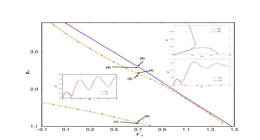
Figure 9: The solid line gives the relation between the expansion factor $F_{\star}$ and the slope $p_{\star}$ of $M^{2}(R)$ at the Alfvén point for a solution through all critical points, for case (b) with parameters: $\epsilon=0.5$, $\xi=-5$, $\delta\nu^{2}=4$, $\delta_{0}\nu^{2}=0.001$, $\mu_{0}=0$. The topologies of $M^{2}(R)$ at the neighboring points (1) to (6) are also shown.

As in case (a), the focusing of the poloidal field/stream lines towards the magnetic and rotation axis is caused predominantly by the magnetic pinching force; this may be seen in the left panel of Fig. (10) where the various components of the forces acting on the plasma perpendicular to the poloidal fieldlines are plotted. In the inner region of the outflow $R$$\buildrel{\scriptstyle<}\over{\scriptstyle\sim}$$1$, the total inertial force perpendicular to the lines (centripetal force) is almost exclusively provided by the inwards magnetic force. In the far zone where gravity is negligible, $R$ $\buildrel{\scriptstyle>}\over{\scriptstyle\sim}$$1$, the inwards magnetic pinching force is balanced by the pressure gradient of the overpressured jet and the centrifugal force. The acceleration of the plasma along the poloidal lines can be seen in the right panel of Fig. (10). In the inner region $R$ $\buildrel{\scriptstyle<}\over{\scriptstyle\sim}$$1$ the magnetic and pressure gradient forces accelerate the plasma; in the outer region where gravity and the magnetic forces are negligible, the pressure gradient force is left alone to accelerate the plasma. As in case (a), it may also be seen in the right panel of Fig. (10) that most of the acceleration occurs in the far region at $R\approx 10$ by the thermal pressure gradient force.
Figure (9) is a plot of the values of $p_{\star}$ and $F_{\star}$ for which the fast point is crossed. As in case (a), we integrate Eqs. (58) - (70) downstream of the Alfvén critical point at which $R=G=M=1$, $F=F_{\star}$, $P_{1}=P_{1\star}$ and $P_{0}=P_{0\star}$. At $R=1$ the Alfvén regularity condition relates $F_{\star}$, $p_{\star}$ and $P_{1\star}$, Eq. (30). Also there is a relation between $F_{\star}$,$p_{\star}$ such that the solution passes through the fast critical point; this is the solid line in Fig. (9). Assume for example that we choose $F_{\star}=0.7$ and we vary $p_{\star}$, Fig. (9). There is only one value of $p_{\star}\approx 2.6$ which satisfies the Alfvén regularity condition and the solution crosses the fast critical point.

For other values of $p_{\star}$ above and below $p_{\star}\approx 2.6$ we have different types of solutions shown in Fig. (9):

• at point (6) of Fig. (9) corresponding to $p_{\star}$ higher than $p_{\star}\approx 2.6$ we get solutions in which the denominator of the differential equation for $M^{2}$ becomes zero and the curve $M^{2}(R)$ turns back to smaller distances,

• at points (5), (4) and (1) of Fig. (9) we get solutions in which the numerator of the differential equation for $M^{2}$ becomes zero and then the solutions become again subAlfvénic,

• at points (2) and (3) of Fig. (9) we get oscillatory solutions wich do not cross the fast critical point. These solutions were shown in figures (7).

A fine tuning between points (6) and (5) gives the unique solution which goes to infinity with superAlfvénic and superfast radial velocity.

Note that in this case there exists a value $\alpha_{out}$ where $V_{\phi}=0$ and $B_{\phi}=0$. In this streamline the enclosed poloidal current is zero. For $\mu=9$ and the parameters as in Fig. (7), $\alpha_{out}=3.24$.

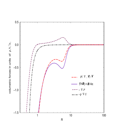
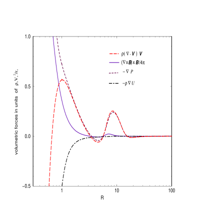
Figure 10: In the left panel are plotted the components of the magnetic (solid), pressure gradient (small dashes), gravitational (dot-dashed) and total acceleration (long dashes) perpendicular to the poloidal streamlines on line $\alpha=\alpha_{lim}$. In the right panel the corresponding components parallel to the poloidal lines are plotted also for case (b) and the same set of parameters: $\epsilon=0.5$, $\xi=-5$, $\delta\nu^{2}=4$, $\delta_{0}\nu^{2}=0.001$, $\mu_{0}=0$, $F_{\star}=1$ and $p_{\star}=2$

Figure 11: Poloidal streamlines close and far from the central object for case (c) with parameters: $\epsilon=2$, $\xi=10$, $\delta\nu^{2}=4$, $\delta_{0}\nu^{2}=0.1$, $\mu_{0}=0$, $F_{\star}=0.8$ and $p_{\star}\approx 2.5636$. The Alfvén (fast) surface is indicated by dashed (dot-dashed) lines.

5.3 Case (c): $\epsilon>1$, $\xi>0$

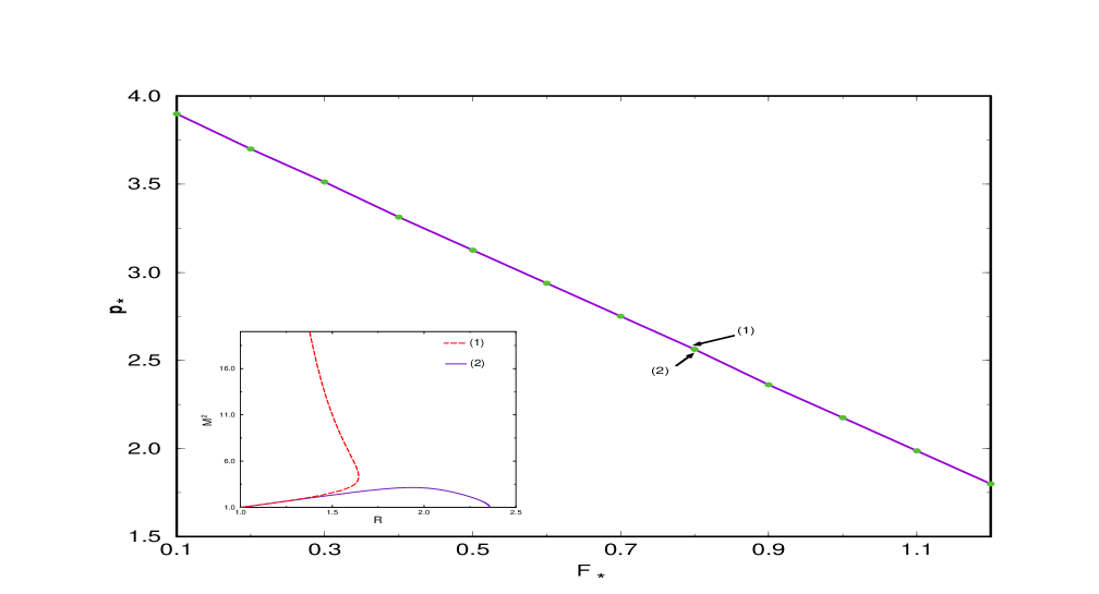
Figure 12: The solid line gives the relation between the expansion factor $F_{\star}$ and the slope $p_{\star}$ of $M^{2}(R)$ at the Alfvén point for a solution through all critical points, for case (c) with parameters: $\epsilon=2$, $\xi=10$, $\delta\nu^{2}=4$, $\delta_{0}\nu^{2}=0.1$, $\mu_{0}=0$.

Figure 13: Dimensionless velocities for case (c) with parameters: $\epsilon=2$, $\xi=10$, $\delta\nu^{2}=4$, $\delta_{0}\nu^{2}=0.1$, $\mu_{0}=0$, $F_{\star}=0.8$ and $p_{\star}\approx 2.5636$.

As discussed in the beginning of Sec. 5, when $\epsilon>1$ the strong magnetic pinching force results in a jet of zero asymptotic radius; in addition, this asymptotics is achieved without oscillations, i.e., we obtain type II solutions, Fig. (12), (11) and (13). The values of $p_{\star}$ and $F_{\star}$ for which the solution crosses the fast critical point are shown in Fig. (12).

As with the previous cases, for each value of $F_{\star}$ there is only one value of the Alfvén number slope $p_{\star}$ such that the solution passes through the fast critical point; this is the solid line in Fig. (12). Assume for example that we choose $F_{\star}=0.8$ and we vary $p_{\star}$, Fig. (12). There is only one value of $p_{\star}\approx 2.53$ which satisfies the Alfvén regularity condition and the solution crosses the fast critical point. For other values of $p_{\star}$ above and below $p_{\star}\approx 2.53$ we have two different types of unphysical solutions shown in Fig. (12):

• at point (1) of Fig. (12) corresponding to $p_{\star}$ higher than $2.53$ we get solutions in which the denominator of the differential equation for $M^{2}$ becomes zero and the curve $M^{2}(R)$ turns back to smaller distances,

• at point (2) of Fig. (12) corresponding to $p_{\star}$ lower than $2.53$ we get solutions in which the numerator of the differential equation for $M^{2}$ becomes zero and then the solutions become again subAlfvénic,

A fine tuning between points (1) and (2) gives the unique solution which goes to infinity with superAlfvénic and superfast radial velocity. Nevertheless, the jet radius goes to zero in this case.

Table 1: Astrophysical applications for cases (a) and (b)

		case (a)					case (b)
		base	Alfvén	fast	infinity		base	Alfvén	infinity
$r(cm)$		$2\times 10^{11}$	$10^{12}$	$2.04\times 10^{12}$	$\gg r_{\star}$		$2\times 10^{11}$	$10^{12}$	$\gg r_{\star}$
$V_{r}(cm/sec)$		$3\times 10^{4}$	$7.7\times 10^{5}$	$1.8\times 10^{6}$	$5\times 10^{7}$		$6.5\times 10^{6}$	$3.2\times 10^{7}$	$10^{8}$
$B_{r}(G)$		$7\times 10^{-3}$	$5.7\times 10^{-4}$	$4\times 10^{-4}$	$10^{-3}$		$0.3$	$6.2\times 10^{-2}$	$10^{-3}$
$\rho(gr/cm^{3})$		$1.6\times 10^{-17}$	$5.1\times 10^{-2}$	$1.5\times 10^{-2}$	$1.66\times 10^{-21}$		$8\times 10^{-18}$	$3.4\times 10^{-19}$	$1.66\times 10^{-21}$
$M^{2}$		$3.2\times 10^{-3}$	$1$	$3.34$	$31.3$		$4.22\times 10^{-2}$	$1$	$203$
$G^{2}$		$8.2\times 10^{-2}$	$1$	$1.41$	$0.477$		$0.206$	$1$	$64$

6 Astrophysical Applications

It should be noted that the purpose of this paper has not been to construct a specific model for a given collimated outflow; instead, our goal has been to outline via a specific class of exact and self-consistent models, the interplay of the various MHD processes contributing into the acceleration and collimation of jets. Nevertheless, the illustrative examples analysed in this paper can be compared with the observable characteristics of outflows from stellar or galactic objects, say, those associated with young stellar objects. For this purpose, in the following we establish the connection between the nondimensional models and the observable parameters of the outflow.

Suppose that at the polar direction of the stellar surface ($r=r_{0}\,,\alpha=0$) we know the values of $V_{r}\,,B_{r}$ and $\rho$, say, $V_{0}$, $B_{0}$ and $\rho_{0}$, respectively, such that we calculate $M_{0}=V_{0}\sqrt{4\pi\rho_{0}}/B_{0}$. From the integration we can find the distance $R_{0}$ where $M(R_{0})=M_{0}$. Thus, we may calculate the Alfvén distance $r_{\star}=r_{0}/R_{0}$. Each line which has its footpoint on the stellar surface at angle $\theta_{i}$ is labeled by $\alpha=\left({r_{0}\sin\theta_{i}}/{r_{\star}G\left(r_{0}/r_{\star}\right)}\right)^{2}$. The last line originating from the star is $\alpha_{lim}$. Each line which has its footpoint on the disk at distance $r_{i}>r_{0}$ from the axis of rotation is labeled by $\alpha=\left({r_{i}}/{r_{\star}G\left(r_{i}/r_{\star}\right)}\right)^{2}>\alpha_{lim}$.
If at the stellar surface $G(R_{0})=G_{0}$ we find the Alfvén values, $V_{\star}=V_{0}G_{0}^{2}/M_{0}^{2}$, $B_{\star}=B_{0}G_{0}^{2}$, $\rho_{\star}=\rho_{0}M_{0}^{2}$ and from Eqs. (26) to (2.4) we can find all physical quantities at any point. For example at $R\gg 1$, $\alpha=0$ we have the following asymptotic values: $V_{\infty}=V_{0}G_{0}^{2}M_{\infty}^{2}/M_{0}^{2}G_{\infty}^{2}$, $B_{\infty}=B_{0}G_{0}^{2}/G_{\infty}^{2}$, $\rho_{\infty}=\rho_{0}M_{0}^{2}/M_{\infty}^{2}\,.$

6.1 Model of case (a)

For a typical solution with parameters as those plotted in Fig. (3), the values of characteristic physical quantities are shown in Table 1. These values refer to the intersection of the rotational axis with (i) the stellar surface, (ii) the Alfvén singular surface, (iii) the modified by the self-similarity fast singular surface and (iv) infinite distance from the source. For a solar type stellar mass $2\times 10^{33}gr$ we have $\nu^{2}=462$ while for $\mu=0.01$ the angular velocity at the equatorial point of the stellar surface has the solar value $2\times 10^{-6}/sec$ .
Note that in this case (a) the toroidal component of the magnetic field changes sign at some spherical surface (cf. the velocity $V_{A\phi\,,lim}$ in Fig. (4). This means that the poloidal current enclosed by this surface is zero. All fieldlines which pass through this surface have the same cylindrical distance from the axis with the Alfvén point ($G=1$ at this spherical surface) while for larger distances $G<1$. After crossing this surface the Poynting flux changes its sign and thus the toroidal component of the velocity becomes large enough (because $V_{\phi}/\varpi\Omega=\left(M^{2}-G^{2}\right)/G^{2}\left(M^{2}-1\right)\approx 1/G^{2}$). It is worth to note that even with such rather weak strengths of the magnetic field, collimation is readily achieved.

6.2 Model of case (b)

For a typical solution with parameters as those plotted in Fig. (7), the values of characteristic physical quantities are also shown in Table 1 and these values refer, as before, to the intersection of the rotational axis with (i) the stellar surface, (ii) the Alfvén singular surface and (iv) infinite distance from the source. The last line connected with the star has $\alpha_{lim}=0.19$ while the disk has a radius $2.45\times 10^{12}cm$. If we choose a one solar mass star, $\nu^{2}=0.3$ while for $\mu=9$, the stellar equator rotates with a speed $2.7\times 10^{4}cm/sec$ (the angular velocity is $1.3\times 10^{-7}/sec$).

The asymptotic radius of the jet (which is bounded with the line $\alpha_{out}$) is $1$ $A.U.$ while the part of the flow starting from the stellar surface has a radius $0.23$ $A.U.$.This part of the jet is collimated at a distance of about $4$ $A.U.$ from the equatorial plane, while the whole solution collimates at a height of $3.3$ $A.U.$ These results are consistent with recent observations of YSO’s (Ray et al 1996).

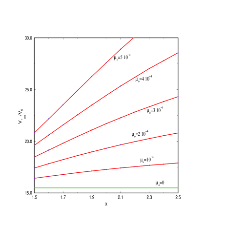
Figure 14: Dimensionless asumptotic values of the radial velocity as a function of the radiative force parameters $x$ and $\mu_{0}$ for case (b) with parameters: $\epsilon=0.5$, $\xi=-5$, $\delta\nu^{2}=4$, $\delta_{0}\nu^{2}=0.001$, $\nu^{2}=0.3$, $F_{\star}=1$ and $p_{\star}=2$. In all these cases in the surface of the star $M_{0}^{2}=4.22\times 10^{-2}$.

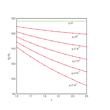
Figure 15: Dimensionless asumptotic values of the radius of the jet as a function of the radiative force parameters $x$ and $\mu_{0}$ for case (b). The other parameters are the same as in the previous figure.

6.3 Model of case (b) including radiation

There are two parameters ($\mu_{0}\,,x$) determining the radiative force (the third is included into $\nu^{2}$). For the parameters of case (b) but for $\mu_{0}\neq 0$ we examine the effect of the radiative force on the velocity and the assymptotic radius of the outflow. As we expect, as the radiative force increases, the terminal velocity becomes larger, Fig. (14) while the Alfvén surface moves closer to the stellar base. From mass conservation we expect that the cross sectional area of the jet decreases as $x$ increases, as it is shown in Fig. (14).

7 Summary and Conclusions

In this paper we have examined a class of exact solutions of the set of the MHD equations (1) - (2) governing the kinematics of a magnetized outflow from a rotating gravitating object. For this system to be closed, an additional equation is needed to describe the energetics of the outflow, i.e., some form of the energy conservation principle, Eq. (3). The often used simplifying polytropic relationship between pressure and density which corresponds to a specific functional form of the net heating/cooling in the plasma, was not used. This has the incovenient consequence that the sound speed is ill defined and it can be calculated only at the critical points. Besides this inconveniency we do not suffer any loss of generality in adopting a more general functional form of the total heating, than the polytropic assumption implies. As it was explained in Sec. 2, in both, the familiar polytropic case of constant $\gamma$ and the present nonconstant $\gamma$ approach, the detailed spatial distribution of the required heating can be calculated only a posteriori.

The class of solutions which is analysed in this paper belongs to a group of nine classes of meridionally selfsimilar MHD solutions which have been shown to exist in the recent paper VT98 under the assumptions that the Alfvén Mach number is a function of the radial distance and the poloidal magnetic field has a dipolar angular dependence, Eq. (7). These assumptions may be reasonable for outflows around the magnetic and symmetry axis of the system. No assumption was made about the asymptotics of the outflows. It is interesting that the self-consistently deduced shape of the streamlines and magnetic field lines was found to be helices wrapped on surfaces which asymptotically are cylindrical. In other words, the streamlines extended to infinite heights above the central object and its disk obtaining the form of a jet. It was shown that such collimation is obtained even with very weak magnitudes of the magnetic field. This result may be contrasted to the quite often refered Blandford & Payne (1982) solutions which by overfocusing towards the axis terminate at finite heights above the disk. The new element the present model introduces in the self consistent modelling of MHD outflows is that it produces for the first time jet-type solutions extending from the stellar base to infinity and where the outflow crosses at a finite distance the fast critical point such that the MHD causality principle is satisfied. The cylindrical asymptotics of the present nonpolytropic solutions are consistent with the polytropic analysis of Heyvaerts & Norman (1989) and also with the class of superAlfvenic but subfast at infinity solutions of Sauty & Tsinganos (1994) for efficient magnetic rotators. However, no radial asymptotics was found in the present class of models, contrary to the other class of meridionally selfsimilar solutions examined in Sauty & Tsinganos (1994) where for inefficient magnetic rotators radial asymptotics has been found; it may be that the present model belongs to the group of efficient magnetic rotators.

The topologies of the solutions are rather rich as it was shown in the plane defined by the slope of the Alfvén number $p_{\star}$ and the streamline expansion factor $F_{\star}$ at the Alfvén transition. For example, for a given streamline expansion factor $F_{\star}$ we obtained terminated solutions for $p>p_{\star}$, similarly to the corresponding terminated solutions in Parker’s (1958) HD wind, or, the Weber & Davis magnetized wind. For a given pressure at the Alfvén point, the requirement that a solution crosses the Alfvén and fast critical points eliminates the freedom in choosing $p_{\star}$ and $F_{\star}$ through the corresponding regularity and criticality conditions.

A plotting of the various forces acting along and perpendicular to the poloidal streamlines reveals that the wrapping of the field lines around the symmetry axis is caused predominantly by the hoop stress of the magnetic field and it is already strong at the Alfvén (and fast) critical surface. Asymptotically the cylindrical column is confined by the interplay of the inwards magnetic pinching force, the outwards centrifugal force and the pressure gradient, as in Trussoni et al (1997). On the other hand, the acceleration of the plasma along the poloidal magnetic lines, in the near zone close to the Alfvén distance it is due to the combination of thermal pressure and magnetic forces while at the intermediate zone beyond the Alfvén point it is basically the pressure gradient that is responsible for the acceleration.

Appendix A functions of $R$

$$F=2-R\frac{G^{2^{\prime}}}{G^{2}}\equiv\frac{\partial\ln\alpha(R,\theta)}{\partial\ln R}\,.$$ (37)

$$f_{1}=-\frac{1}{G^{4}}\,,$$ (38)

$$f_{2}=-\frac{F^{2}-4}{4G^{2}R^{2}}\,,$$ (39)

$$f_{3}=-\frac{1}{G^{2}}\left(\frac{1-G^{2}}{1-M^{2}}\right)^{2}\,,$$ (40)

$$f_{4}=\frac{F}{2RG^{2}}M^{2^{\prime}}-\frac{1-M^{2}}{2RG^{2}}F^{{}^{\prime}}-\frac{\left(1-M^{2}\right)F\left(F-2\right)}{4R^{2}G^{2}}\,,$$ (41)

with,

$$F^{\prime}=\frac{F}{1-M^{2}}M^{2^{\prime}}-\frac{F\left(F-2\right)}{2R}-\frac{2RG^{2}}{1-M^{2}}f_{4}\,,$$ (42)

$$f_{5}=\frac{G^{4}-M^{2}}{G^{2}M^{2}\left(1-M^{2}\right)}\,,$$ (43)

$$f_{6}=-\frac{2}{G^{4}}M^{2^{\prime}}+\frac{2\left(1-M^{2}\right)\left(F-2\right)}{RG^{4}}\,,$$ (44)

$$f_{7}=\frac{2}{R^{2}G^{2}}M^{2^{\prime}}-\frac{\left(1-M^{2}\right)\left(F-2\right)\left(F+4\right)}{2R^{3}G^{2}}-\frac{F}{R}f_{4}\,,$$ (45)

$$f_{8}=-\frac{F-2}{R}f_{5}\,,$$ (46)

$$f_{9}=\frac{2}{M^{2}}\left(Q-\frac{\nu^{2}}{2R^{2}}\right)\,.$$ (47)

Appendix B physical quantities and differential equations of model

The MHD integrals have the following forms,

$$\Psi_{A}=\sqrt{4\pi\rho_{\star}\left(1+\delta\alpha+\mu\delta_{0}\alpha^{\epsilon}\right)}\,,$$ (48)

$$\Omega=\frac{V_{\star}}{r_{\star}}\sqrt{\frac{\mu\alpha^{\epsilon-1}+\xi}{1+\delta\alpha+\mu\delta_{0}\alpha^{\epsilon}}}\,,$$ (49)

$$L=V_{\star}r_{\star}\sqrt{\frac{\mu\alpha^{\epsilon+1}+\xi\alpha^{2}}{1+\delta\alpha+\mu\delta_{0}\alpha^{\epsilon}}}\,.$$ (50)

The three ordinary differential equations for the functions of $R$ are

$$\left.\begin{array}[]{r}f_{0}^{{}^{\prime}}-f_{6}-f_{9}=0\\ f_{4}^{{}^{\prime}}-f_{7}+\xi\left(f_{5}^{{}^{\prime}}-f_{8}\right)-\delta f_{9}=0\\ \mu\left(\frac{f_{5}^{{}^{\prime}}}{\epsilon}-f_{8}-\delta_{0}f_{9}\right)=0\end{array}\right\}$$ (51)

or using the definitions of $P_{0}\,,P_{1}$ and $F$

$$\begin{array}[]{l}\displaystyle{{dG^{2}\over dR}=-{{F-2}\over R}G^{2}}\,,\end{array}$$ (52)

$$\begin{array}[]{l}\displaystyle{\frac{dF}{dR}=\frac{F}{1-M^{2}}\frac{dM^{2}}{dR}-\frac{F\left(F-2\right)}{2R}-}\\ \\ \displaystyle{\frac{F^{2}-4}{2R\left(1-M^{2}\right)}-\frac{2G^{2}RP_{1}}{1-M^{2}}-}\\ \\ \displaystyle{\frac{2\xi R}{M^{2}\left(1-M^{2}\right)^{3}}\left[\left(2M^{2}-1\right)G^{4}-M^{4}+2M^{2}\left(1-G^{2}\right)\right]}\end{array}$$ (58)

$$\begin{array}[]{l}\displaystyle{\frac{dM^{2}}{dR}=\frac{M^{2}\left(1-M^{2}\right)}{\left(2M^{2}-1\right)G^{4}-M^{4}}\left\{2\epsilon\delta_{0}G^{2}\left(1-M^{2}\right)\left(Q-\frac{\nu^{2}}{2R^{2}}\right)+\right.}\\ \\ \displaystyle{\left.\frac{F-2}{R}\left[\left(\epsilon+1\right)M^{2}-\left(\epsilon-1\right)G^{4}\right]\right\}}\end{array}$$ (62)

$$\begin{array}[]{l}\displaystyle{\frac{dP_{1}}{dR}=-\left[\frac{F^{2}-4}{2R^{2}G^{2}}+2\xi\frac{\left(1-G^{2}\right)^{2}}{G^{2}\left(1-M^{2}\right)^{3}}\right]\frac{dM^{2}}{dR}-}\\ \\ \displaystyle{\frac{M^{2}F}{2R^{2}G^{2}}\frac{dF}{dR}+\frac{2\delta}{M^{2}}\left(Q-\frac{\nu^{2}}{2R^{2}}\right)-\frac{M^{2}\left(F^{2}-4\right)\left(F-4\right)}{4R^{3}G^{2}}+}\\ \\ \displaystyle{\xi\frac{\left(F-2\right)\left[\left(2M^{2}-1\right)G^{4}-M^{4}\right]}{RG^{2}M^{2}\left(1-M^{2}\right)^{2}}}\end{array}$$ (68)

$$\begin{array}[]{l}\displaystyle{\frac{dP_{0}}{dR}=-\frac{2}{G^{4}}\frac{dM^{2}}{dR}+\frac{2}{M^{2}}\left(Q-\frac{\nu^{2}}{2R^{2}}\right)-\frac{2M^{2}\left(F-2\right)}{RG^{4}}}\end{array}$$ (70)

The pressure component $P_{2}(R)$ is given explicitly in terms of the other variables:

$$P_{2}=\frac{\mu}{G^{2}}\left[\frac{G^{4}-M^{2}}{\epsilon M^{2}\left(1-M^{2}\right)}-\left(\frac{1-G^{2}}{1-M^{2}}\right)^{2}\right]\,.$$ (71)

The functional form of the pressure, Eq. (27), corresponds to the following functional form for the heating function

$$\frac{q}{\rho V_{r}}=\frac{V_{\star}^{2}}{2r_{\star}}\frac{{\cal Q}_{0}+{\cal Q}_{1}\alpha+{\cal Q}_{2}\alpha^{\epsilon}}{1+\delta\alpha+\mu\delta_{0}\alpha^{\epsilon}}$$ (72)

with ${\cal Q}_{i}=M^{-2\left(\Gamma-1\right)}\displaystyle{\frac{d}{dR}\left(\frac{M^{2\Gamma}P_{i}}{\Gamma-1}\right)}\,,i=0,1,2$. As discussed in Sec. 2.1, one could proceed in the reverse way, i.e., to start with the functional form of the heating function and deduce the functional form of the pressure Eq. (27).

References

- [1] Biretta, T., 1996, in Solar and Astrophysical MHD Flows, K. Tsinganos (ed.), Kluwer Academic Publishers, 357
- [2] Blandford, R.D., Payne, D.G., 1982, MNRAS, 199, 883 (BP82)
- [3] Bogovalov, S.V., 1996, MNRAS, 280, 39
- [4] Bogovalov, S.V., Tsinganos, K., 1999, MNRAS, (in press)
- [5] Chen, H, Marlborough, J.M., 1994, ApJ, 427, 1005
- [6] Contopoulos, J., Lovelace, R.V.E., 1994, ApJ., 429, 139
- [7] Ferrari, A., Massaglia, S., Bodo, G., Rossi, P., 1996, in Solar and Astrophysical MHD Flows, K. Tsinganos (ed.), Kluwer Academic Publishers, 607
- [8] Ghosh, P., Lamb, F.K., 1979, ApJ, 234, 296
- [9] Goodson, A.P., Winglee, R.M., Bohm, K.H., 1997, ApJ, 489, 199
- [10] Heyvaerts, J., Norman, C.A., 1989, ApJ, 347, 1055
- [11] Kahabka, P., Trumper, J., 1996, in Compact Stars in Binaries, E.P.J. Van den Heuvel & J. van Paradijs (eds.), (Dordrecht: Kluwer), p. 425
- [12] Kakouris, A., Moussas, X., 1997, A&A, 324, 1071
- [13] Lamers, H.J.G.L.M., 1986,AA, 159, 90
- [14] Livio, M., 1997, in Accretion Phenomena and Related Outflows, D.T. Wickramasinghe, L. Ferrario, & G.V. Bicknel (eds.), ASP: San Francisco, 845.
- [15] Low, B.C., Tsinganos, K. 1986, ApJ, 302, 163
- [16] Mirabel, I.F., Rodriguez, L.F., 1996, in Solar and Astrophysical MHD Flows, K. Tsinganos (ed.), Kluwer Academic Publishers, 683
- [17] Ostriker, E.C., 1997, ApJ, 486, 291
- [18] Ouyed, R., Pudritz, R.E., 1997a, ApJ, 482, 712
- [19] Ouyed, R., Pudritz, R.E., 1997b, ApJ, 484, 794
- [20] Parker, E.N. 1958, ApJ, 128, 664
- [21] Ray, T.P., 1996, in Solar and Astrophysical MHD Flows, K. Tsinganos (ed.), Kluwer Academic Publishers, 539
- [22] Ray, T.P., Mundt, R., Dyson, J.E., Falle, S.A.E., Raga, A., 1996, ApJ, 468, L103.
- [23] Sakurai, T. 1985, A&A, 152, 121
- [24] Sauty, C., Tsinganos, K., 1994, A&A, 287, 893
- [25] Shahbaz, T., Livio, M., Southwell, K.A., Charles, P.A., 1997, ApJ, 484, L59
- [26] Trussoni, Tsinganos, K., E., Sauty, C., 1997, A&A, 325, 1099
- [27] Tsinganos, K.C., 1982, ApJ, 252, 775
- [28] Tsinganos, K., Trussoni, E., Sauty, C., 1992, in The Sun: A Laboratory for Astrophysics , J.T. Schmelz and J. Brown (eds.), Kluwer Academic Publishers, 349
- [29] Tsinganos, K., Sauty, C., Surlantzis, G., Trussoni, E., Contopoulos, J., 1996, MNRAS, 283, 811
- [30] Uchida, Y., Shibata, K., 1985, PASJ, 37, 515
- [31] Ustyugova, G.V., Koldoba A.V., Romanova M.M., Chechetkin V.M., Lovelace, R.V.E., 1999, ApJ, (in press)
- [32] Vlahakis, N., Tsinganos, K., 1997, MNRAS, 292, 591 (VT97)
- [33] Vlahakis, N., Tsinganos, K., 1998, MNRAS, 298, 777 (VT98)
- [34] Weber, E.J., Davis, L.J. 1967, ApJ, 148, 217