A New Weak Lensing Analysis of MS1224.7+2007

Abstract

Galaxy cluster mass distributions are useful probes of $\Omega_{0}$ and the nature of the dark matter. Large clusters will distort the observed shapes of background galaxies through gravitational lensing allowing the measurement of the cluster mass distributions. For most cases, the agreement between weak lensing and radial velocity mass measurements of clusters is reasonably good. There is, however, one significant exception, the $z=0.32$ cluster MS1224+2007, which has a lensing mass substantially larger than the virial mass and also a very high mass-to-light ratio. Since this controversial object might be an unusually dark mass a follow-up study is definitely warranted.

In this paper we study the mass and light distributions of MS1224+2007 out to a projected radius of 800 $h^{-1}$ kpc by measuring the gravitationally-induced distortions of background galaxies. We detect a shear signal in the background galaxies in the radial range $27.5\arcsec\ \leq r\leq 275\arcsec$ at the 5.5$\sigma$ level. The resultant mass map exhibits a peak centered on the dominant cluster galaxy and strong evidence for substructure which is even more strongly seen in the galaxy distribution. Assuming all the detected shear is due to mass at $z=0.32$ we find cluster mass-to-light ratio of M/L${}_{R}=640\pm 150$ (M/L${}_{R})_{\odot}$. The mass profile is quite flat compared to other clusters, disagreeing with a pseudo-singular isothermal sphere at the 95% confidence level. Our mass and M/L estimates are consistent with the previous weak lensing result. The discrepancy between the lensing and virial mass remains although it might be partially explained by subclustering and infall perpendicular to the line-of-site. This cluster remains a candidate dark object deficient in baryons and as such severely tests cosmological models.

1 Introduction

Weak lensing distortions of background galaxies are a powerful tool for measuring galaxy cluster mass distributions. Lensing based studies are direct measurements and are not model-dependent as are other techniques (X-ray, radial velocities). Currently there are around 20 clusters which are well-studied with lensing (e.g. Fischer & Tyson (1997)), most yielding an evolution corrected M/L$\approx 300$ (M/L)_⊙.

There is, however, one significant exception, the z=0.32 cluster MS1224+2007, which has M/L = 800 (M/L$)_{\odot}$ from the weak lensing measurements of Fahlman et al. (1994). Not only is the lensing-derived M/L estimate very high but the mass estimate is approximately a factor of 2.5 higher than the virial mass estimate (Carlberg et al. (1994)). If the lensing mass is correct then it would indicate a large region with an anomolously low baryon fraction. Within the standard cosmological model there is no causal mechanism which can generate primordial fluctuations in the baryon-to-total mass ratio on cluster scales (Evrard (1997)). Furthermore, dynamical processes operating differentially on the baryonic and dark matter do not appear able to cause variations at the implied level (i.e. Metzler & Evrard (1994)).

In general, clusters are found based on their optical appearance and/or their X-ray emission, which are both baryonic in origin. However, baryons are a small component of the total cluster mass ($0.060\pm 0.003h^{-3/2}$, Evrard (1997)). Therefore, clusters may be very biased locations; measurements made in these regions may not be representative of the whole universe. Are clusters special places where there just happens to be large amounts of baryonic matter? Are there massive objects containing little or no baryonic matter which we have yet to detect? Is MS1224 an example of such a dark object? If so, this would represent a significant challenge for theories of large-scale structure formation and might also imply that estimates of $\Omega_{0}$ based on cluster masses are underestimated.

It is, therefore, important to confirm the weak lensing mass measurement of MS1224+2007 with an independent study. In this paper we present a weak lensing study of MS1224+2007 carried out with the MDM 2.4m. The observations and reductions are described in §2 and §3. The shear and mass measurements are described in §4 and §5 along with comparisons with previous lensing and virial mass estimates. Conclusions and future work are presented in §6

2 Observations

The cluster MS1224+2007 was observed using with Michigan-Dartmouth-MIT (MDM) 2.4m telescope on 8-9 Feb. 1998. The total exposure time was 21600s in R ($41\times 900$s) and 4500s in B ($5\times 900$s). The telescope was dithered between exposures. The “Echelle” 2048² thinned SITe CCD was used with 0.275″ pixels. The seeing on the combined R image is 0.9″ FWHM and 1.4″ for the combined B image. The RMS sky noise values are 28.0 B mag per square arcsecond and 28.1 R mag per square arcsecond. The two nights were not perfectly photometric, the sky transparency varied by 9% as determined from monitoring 50 stars in the field of MS1224+2007 (due to occasional small clouds passing through the field of view). We scale each image to match the flux of the highest throughput images.

Despite the variations in sky transparency, 50 standard stars (Landolt (1992)) were measured over the two nights. Transformation functions with linear color and airmass terms are fit to the data resulting in an RMS of 0.03 mag and 0.013 mag for the B and R data respectively while the color terms are 0.035 and 0.013, respectively. Since the R-band data is much deeper than the B-band data and the color terms are very small, we calibrate the data assuming a mean galaxy color of $\langle$B–R$\rangle$=1.6. This introduces errors of $\pm 0.05$ and $\pm 0.02$ for the B and R photometry respectively.

The reddening in this field is E(B-V)=0.04 yielding A${}_{B}=0.17$ and A${}_{R}=0.11$ (Schlegel et al. (1998)).

3 Faint Galaxy Photometry and Analysis

The faint galaxy analysis was carried out using the analysis software ProFit (developed by the author). This software, starting with the brightest detections, fits an analytical model to each object using weighted, non-linear least squares, and subtracts the light from the image. It then proceeds to successively fainter objects. Once it has detected and subtracted all the objects in an image it replaces each in turn and refits and resubtracts until convergence is achieved. The software outputs brightness, orientation, ellipticity and other image parameters based on the fitted function.

4 Gravitational Shear

4.1 Theory

For gravitational lensing, the relationship between the tangential shear, $\gamma_{T}$, and surface mass density, $\Sigma$, is (Miralda-Escudé (1991), Miralda-Escudé (1995)),

$$\gamma_{T}(r)=\overline{\kappa}(\leq r)-\overline{\kappa}(r),$$ (1)

where $\kappa=\Sigma/\Sigma_{crit}$, the ratio of the surface density to the critical surface density for multiple lensing, and $r$ is the angular distance from a given point in the mass distribution. The critical density depends on the redshift distribution of the background galaxies. The first term on the right is the mean density interior to $r$ and the second term is the mean density at $r$. Therefore, the presence of a foreground mass distribution will distort the appearance of background galaxies. For a given coordinate on the image ($\vec{r}$), the distortion quantity for the i^th galaxy is:

$$D_{i}(\vec{r})={1-(b_{i}/a_{i})^{2}\over 1+(b_{i}/a_{i})^{2}}\times{[\cos(2\theta_{i})(\Delta{x_{i}}^{2}-\Delta{y_{i}}^{2})+2\sin(2\theta_{i})\Delta{x_{i}}\Delta{y_{i}}]\over\Delta{x_{i}}^{2}+\Delta{y_{i}}^{2}},$$ (2)

where $(b_{i}/a_{i})$ and $\theta_{i}$ are the galaxy axis ratio and position angle, respectively. $\Delta x$ and $\Delta y$ are the horizontal and vertical angular distances from $\vec{r}$ to galaxy $i$. $D$ is related to the tangential shear by (Seitz & Schneider (1995)):

$$<D(r)>=2{\gamma_{T}(r)[1-\kappa(r)]\over[1-\kappa(r)]^{2}+\gamma_{T}^{2}(r)}$$ (3)

In the weak lensing regime $\kappa<<1$, and $\gamma_{T}<<1$, $\gamma_{T}\approx<D>/2$.

Before proceeding to a discussion of the shear measurments we discuss sources of systematic errors.

4.2 Point-Spread Function Anisotropy

In Figure 1 the ellipticity and orientation for 87 stars with $16.4\leq$ R $\leq 22.3$ in the combined R-band image are shown. There is a strong anisotropy present in the point spread function (PSF) which, if not corrected for, could bias estimates of the shear due to the cluster. We correct for the PSF anisotropy using the method outlined in Fischer & Tyson (1997), which involves deriving a position dependent kernel which, after convolution with the image, yields round PSFs. Figure 1 shows the ellipticity and orientation for the same stars after the correction. We discuss the effects of PSF anisotropy on the shear and cluster mass estimates in §4.5 and §5.2

Figure 1: Ellipticity and orientation for 87 stars in the combined R-band image. The lower panel is the original image and the upper panel is after correction (see text). The maximum ellipticity is $\epsilon=0.07$ and the medians are $<\epsilon>=0.035$ and $0.013$, for the original and corrected, respectively. North is up and East is to the left.

4.3 Seeing and Shear Polarizability

In order to measure the cluster mass using weak gravitational lensing we must measure the shapes of background galaxies to estimate the shear (see §4.1). Even perfect galaxy measurements will result in biased shear estimates for two reasons. The first is that the galaxy ellipticities will be underestimated due to blurring by atmospheric seeing. The second is that the response of a galaxy to a shear will depend on its ellipticity and orientation with respect to the shear and hence the mean response will depend on the intrinsic ellipticity distribution of the galaxies. In order to calibrate these effects we carry out simulations using the F606W Hubble Deep Field Data (HDF) (Williams et al. (1996)), using the techniques described in Kaiser et al. (1995). This involves stretching the HDF data by $1+\delta$, convolving with the PSF and adding noise. The values of $D_{i}$ (see Equation 2) are measured for each galaxy and compared to the unsheared values of $D_{i}$. The quantity of interest is the recovery factor, $C=\delta/<\Delta{D_{i}}>$ which is $<C>=2.76\pm 0.2$ for the present data (galaxies with $22.25\leq$R$\leq 24.0$ are used for the shear analysis, see below). This correction does not take into account the presence of stars which will further dilute the signal, however, this will be minor for the magnitude range considered.

4.4 Cluster Galaxies

Including cluster galaxies in the shear measurment will reduce the measured value of the shear (assuming cluster galaxies are randomly aligned) by an amount equal to the contamination fraction. This effect is likely to be a function of radius since we expect the cluster galaxies to be centrally concentrated within the cluster. For the shear analysis in this paper we use galaxies in the range $22.25\leq$R$\leq 24.0$. In order to get an estimate of the number of cluster galaxies in this brightness range we assume that the contamination is zero at the edge of our image. We then simply measure the density of galaxies in our sample as a function of radius and fit a straight line. This analysis reveals that at a radius of 27.5″ about 22% of the galaxies in our field sample are probably cluster galaxies falling to zero (by construction) at 275″. We adopt this correction for the rest of the paper. If there are a significant number of cluster galaxies at the edge of the image then this correction will be too small and we will be underestimating the shear due to the cluster.

4.5 Measurements

The value of the mean distortion, $<D(\vec{r})>$, for $\vec{r}$ equal to the position of the central dominant galaxy (CDG) in MS1224+2007 for 874 galaxies in the combined R image having $22.25\leq$ R$\leq 24.0$ in the radial range $27.5\arcsec\ \leq r\leq 275\arcsec$ is $<D_{raw}>=0.034\pm 0.006$; the signal-to-noise is 5.5. After correction for blurring by the PSF and shear polarizability (see §4.3) the value is $<D_{cor}>=0.094\pm 0.017$ For comparison, the value of $<D(\vec{r})>$ for $\vec{r}$ at the CDG location for the 87 PSF stars in the corrected image is $0.0009\pm 0.002$, consistent with zero and less than 3% of $<D_{raw}>$. Given that the PSF-induced distortion on the resolved galaxies is actually smaller than this, the residual PSF anisotropy has little effect on our cluster mass estimate.

Figure 2 shows $<D(\vec{r})>$ (corrected, for seeing, shear polarizability and contamination by cluster galaxies) vs. projected radius for $\vec{r}$ at the CDG position. The shear profile is very flat, the best fit singular pseudo-isothermal sphere (SPIS) shown in Figure 2 is ruled out at the 95% confidence level ($\chi^{2}=17.07$, nine degrees of freedom). If we restrict ourselves to nonsingular pseudo-isothermal spheres (NPIS) of form:

$$\Sigma(R) = {\Sigma_{0}\over[1+(R/Rc)^{2}]^{1/2}},$$ (4)

then the best fit model has a core $R_{c}=45^{+25}_{-15}\arcsec=135^{+65}_{-45}h^{-1}$ kpc ($\chi^{2}=10.43$, nine degrees of freedom), and a central surface density $\kappa(0)=0.30\pm 0.055$. The 95% confidence limits on $r_{c}$ are 60 - 400 $h^{-1}$ kpc.

Figure 2: A plot of the distortion, $<D>$, vs projected radius in radial bins containing 87 galaxies each (outermost bin has 91) with $27.5\arcsec\ \leq r\leq 275\arcsec$ and $22.25\leq R\leq 24.0$, centered on the dominant cluster galaxy. The points are from the data ($1\sigma$ error bars) and the lines are the expected distortion for two mass models. The dashed line is a SPIS while the solid line is a NPIS with a core radius of $r_{c}=45\arcsec=135h^{-1}$ kpc. A recovery factor of $C=2.76$ (see text) has been applied along with a correction for contamination by cluster galaxies.

In order to convert the density profile into physical mass units we must know the value of $\Sigma_{crit}$ which requires knowledge of the redshift distribution of the background galaxies. There is no current redshift survey complete to R = 24.0 (actually R = 23.9 because of reddening). We can get an upper limit on $\Sigma_{crit}$ by using the redshifts from the Canada France Redshift Survey (CFRS) (Lilly et al. (1995)). We derive R-band magnitudes by simple averaging of their V and I photometry which should be accurate to 0.1-0.2 mag (Fukugita et al. (1995)). Integrating $\Sigma_{crit}$ over the redshift distribution for $22.25\leq$ R $\leq 24.0$ yields $\langle\Sigma_{crit}\rangle=1.50h$ ($\Omega_{0}=1.0$) and a mean redshift $\langle z\rangle=0.69$. The value of $\Sigma_{crit}$ will be an overestimate since the CFRS survey is incomplete for much of this magnitude range. We perform a similar test with the deeper but smaller Hawaii Deep Field Redshift Survey (interpolating R = 1/3B + 2/3I) and obtain $\langle\Sigma_{crit}\rangle=1.49h$ and a mean redshift $\langle z\rangle=0.69$, although once again this survey is not complete over the entire magnitude range. Another approach which should be somewhat less sensitive to incompleteness at the faint end is to simply calculate the value of $\Sigma_{crit}$ for an object at z = 0.69 (which is the mean of both the redshift surveys). This yields $\Sigma_{crit}=1.35h$. Finally we can use theoretical models of galaxy formation and evolution to extrapolate the known redshift distribution to fainter magnitudes. Adopting the model of Gronwall (1996) we find $\langle z\rangle=0.73$ and $\langle\Sigma_{crit}\rangle=1.44h$ for the relevant reddening-corrected magnitude range. Given the numbers above we adopt $\Sigma_{crit}=1.44h$ with an uncertainty of around 10%.

5 Cluster Mass

5.1 Mass reconstruction

In the weak lensing regime, where $\kappa<<1$, the formula for the surface mass density is (Kaiser & Squires (1993)):

$$\kappa(\vec{r})={1\over\overline{n}\pi}\sum_{i=1}^{N}{W(\Delta{x},\Delta{y},s)D_{i}(\vec{r})\over\Delta{x_{i}}^{2}+\Delta{y_{i}}^{2}}.$$ (5)

where $N$ is the number of galaxies and $\overline{n}$ is the number density of galaxies. Eqn. 5 assumes that the galaxies are intrinsically (in the absence of lensing) randomly aligned. $W$ is a smoothing kernel which is required to prevent infinite formal error. In this paper we use a smoothing kernel of the form (Seitz & Schneider (1995)):

$$W(\Delta{x},\Delta{y},s)=1-\left(1+{\Delta{x}^{2}+\Delta{y}^{2}\over 2s^{2}}\right)e^{-(\Delta{x}^{2}+\Delta{y}^{2})/2s^{2}},$$ (6)

where ‘$s$’ is referred to as the “smoothing scale”. The variance in the dimensionless surface mass density is:

$$\langle\kappa^{2}\rangle={\langle\gamma^{2}\rangle\over 8\pi\overline{n}s^{2}}.$$ (7)

2-d mass maps of MS1224+2007 are shown in Figure 3 and are discussed further in §5.2.

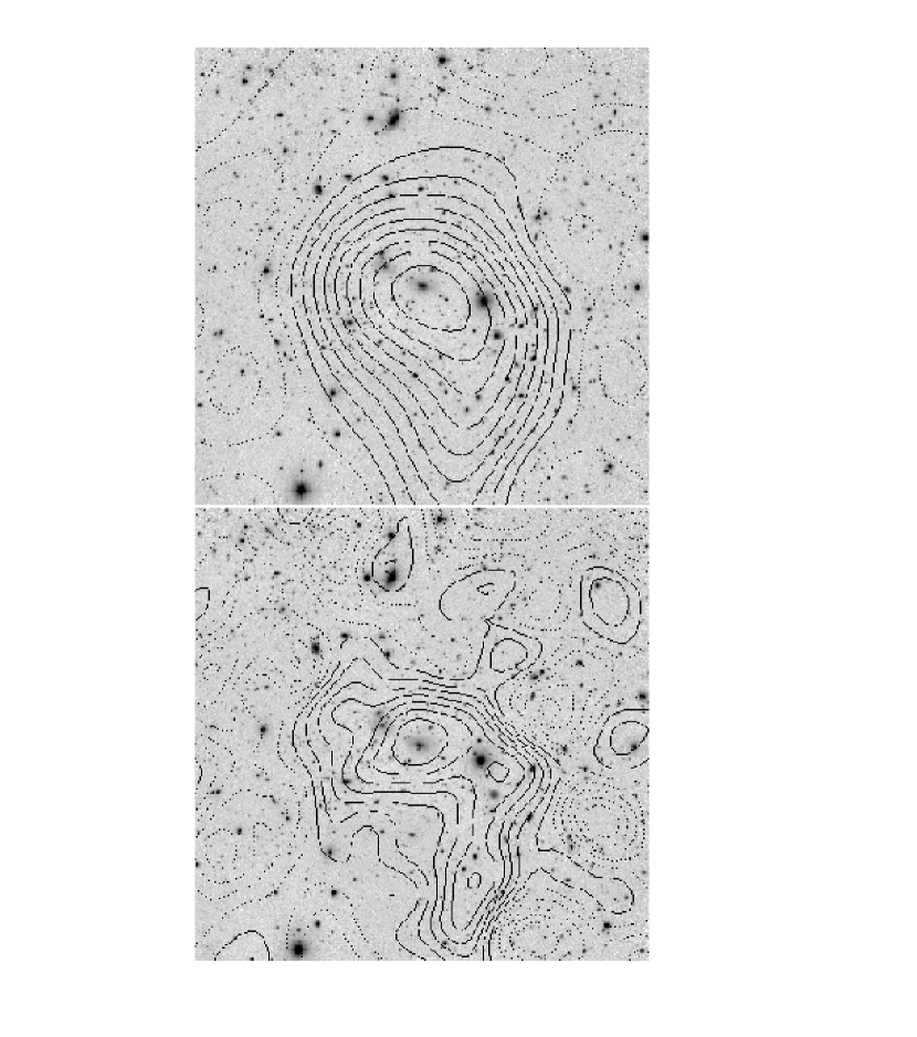
Figure 3: Mass maps derived using Eqn. 5 with smoothing scale $s=60\arcsec$ (top) and $s=30\arcsec$ (bottom). A total of 1201 galaxies with $22.25\leq$ R $\leq 24.0$ are used in these reconstructions. The contours are spaced in 1$\sigma$ intervals. The peak of the mass distribution is consistent with the position of the central dominant galaxy. North is up and East is to the left. The field is 9.6′ on a side.

Because of the smoothing kernel, plus biases introduced by edge effects in the images, Eqn 5 is mainly useful for determining the 2-d shapes of mass distributions. A less biased way of obtaining mass estimates as well as azimuthally averaged density profiles is:

$$\overline{\kappa}(r\leq r_{i})-\overline{\kappa}(r_{i}\leq r\leq r_{o})={r_{o}^{2}\over N_{io}}\sum_{r_{i}\leq r\leq r_{o}}{[1-\kappa(\vec{r})][1-\sqrt{1-D_{i}(\vec{r})^{2}}]\over D_{i}(\vec{r})(\Delta{x_{i}}^{2}+\Delta{y_{i}}^{2})}$$ (8)

where $N_{io}$ is the number of galaxies between $r_{i}$ and $r_{o}$. This is similar to the form employed by Fahlman et al. (1994) but is valid when $\kappa$ is not vanishingly small. Since $\kappa$ appears on the right hand side of the equation, an iterative approach must be used to obtain the density profile. Radial mass profiles for MS1224+2007 are shown in Figure 4 and are discussed further in §5.3.

Figure 4: The upper panel is the radial mass density profile (points) for MS1224+2007 from Eqn. 8 assuming $\kappa=0$ ($r_{o}=275\arcsec\ =790h^{-1}$ kpc). It is centered on the central dominant galaxy. The points are the data for the cluster derived from 874 galaxies having $22.25\leq$ R$\leq 24.0$. The lower panel is the radial density profile from Eqn. 8 using $\kappa$ derived from the best fit to the shear shown in Fig. 2. The value of $r_{o}$ is 275″. A recovery factor of $C=2.76$ (see text) has been applied. The solid lines are the best NPIS model fits to the shear measurments shown in Figure 2.

Galaxy distortion is insensitive to flat sheets of mass. Consequently, all mass measurements described in this paper are uncertain by an unknown additive constant. If there is a substantial flat component to the mass distribution our mass estimates will be lower limits.

5.2 2-d Mass and Galaxy Maps

The 2-d, KS mass map for MS1224+2007 is shown in Figure 3 superposed on the R-band image of the field. This reconstruction uses 1201 galaxies with $22.25\leq$ R$\leq 24.0$. Before discussing the mass distribution we check for potential biases introducecd by residual PSF anisotropies by making a map with the 87 stars from the corrected image. The highest value in this map is 8% of peak value in the cluster map (equal to the 1.0$\sigma$ noise level of the mass map) and therefore all but the lowest couple of contour levels should be unaffected by residual PSF anisotropy. For comparison a map made from the same stars on the uncorrected image had a peak value five times higher.

The mass distribution is peaked very near the position of the CDG and exhibits an extension towards the south. In the higher resolution map this extension appears as a distinct subcluster although its proximity to the edge of the frame makes this conclusion uncertain. An additional subcluster appears to the west of the CDG. This mass maps differs somewhat from the map of Fahlman et al. (1994). The peak of their mass distribution is centered east of the CDG and appears to be extended to the North.

In Figures 5 and 6 we show maps of the galaxy number density and flux-weighted number density, respectively for two R-band magnitude ranges (smoothed to match the high-resolution mass map). The bright number density map is peaked slightly to the east of the CDG while the faint map seems to have a concentration to the southwest of the CDG and a marginal signal in the south. Both show evidence for significant galaxy clustering in the northern portion of the field. The bright flux-weighted map appears to be bimodal with two similar sized luminosity concentrations. One is centered very close to the CDG (not surpising given the brightness of the CDG) and one is to the west. The faint flux-weighted map looks a lot like the faint number density map with a concentration to the southwest of the CDG and a significant feature to the north and a less significant feature to the south.

It is difficult to draw strong conclusions from these maps without redshift information. However, the bimodal central feature seen in both of the bright galaxy maps and in the mass map seems to indicate that there is significant subclustering within the cluster. Furthermore, there is strong evidence for a large concentration of galaxies to the north. Because this concentration is seen more prominently in the faint galaxies and is not seen (or marginally seen) in the massmap it is likely that it is at a higher redshift than $z=0.325$.

Figure 5: Galaxy number density for galaxies in the range $17.28\leq$ R $\leq 22.25$ (upper panel) and $22.25\leq$ R $\leq 23.75$ (lower panel). Both have been smoothed with a Gaussian having a scale of 30″. The contours are spaced in 1$\sigma$ steps which corresponds to 1.2 and 1.3 per square arcmin for the upper and lower panels, respectively

Figure 6: Galaxy luminosity weighted number density for galaxies in the range $17.28\leq$ R $\leq 22.25$ (upper panel) and $22.25\leq$ R $\leq 23.75$ (lower panel). Both have been smoothed with a Gaussian having a scale of 30″. The contours are spaced in 1$\sigma$ steps which corresponds to 21.5 mag per square arcsecond (R-band reddening corrected) and 24.5 mag per square arcsecond for the upper and lower panels, respectively

5.3 Mass and Luminosity Profiles

In the upper panel of Figure 4 we show the azimuthally averaged surface mass density profile centered on the CDG as derived from Equation 8 using 874 galaxies having 22.25 $\leq$R$\leq 24.0$. We have assumed that $\kappa=0$ on the right hand side of the equation. The bottom panel shows the density profile corrected using the best fit values of $\kappa$ from the fits of a NPIS to the shear (see §4). The data have been corrected for seeing, shear polarizability and contamination by cluster galaxies.

Figure 7 shows the mass density profile overplotted with the rest frame R-band surface brightness profile. The surface brightness profile includes light in galaxies with R $\geq 17.28$ (the magnitude of CDG) but does not include possible diffuse light unassociated with galaxies. It is plotted as a density contrast for comparison with the mass density profile. Aside from the innermost regions where the light is completely dominated by the the CDG, it appears that mass traces light. We have applied a K correction to the R-band photometry assuming the cluster light is dominated by early type galaxies of K${}_{cor}=0.4$ (Poggianti (1997)) and an extinction correction of A${}_{R}=0.11$ (Schlegel et al. (1998)). The mass and light profiles are flatter than has been seen for other clusters. Of course, subclustering will cause the azimuthally averaged mass and light profiles to flatten out.

Figure 7: Plot of projected cluster mass density (points) and projected rest-frame R-band luminosity density (solid line) in galaxies. Both are plotted as density contrasts. The dotted line is the best pseudo-isothermal plus core model fit to the shear measurments shown in Figure 2.

Figure 8 shows the cumulative mass and luminosity profiles and Figure 9 shows M(r)/L_R(r) as a function of radius. Within 100 $h^{-1}$ kpc of the CDG the M/L is typical of cluster galaxies ($225\pm 50$ (M/L${}_{R})_{\odot}$). However, beyond the region where the CDG light dominates, the M/L increases rapidly and levels off. Ignoring the first and last points, M/L${}_{R}=640\pm 150$ (M/L${}_{R})_{\odot}$ (M${}_{R\odot}=4.31$) which is an unusually high value. Assuming the cluster is dominated by early-type galaxies, the evolutionary correction to $z=0$ is -0.363 mag (Poggianti (1997)) which yields M/L${}_{R}=890\pm 200$ (M/L${}_{R})_{\odot}$. The typical color of a nearby early-type galaxy is (B-R) = 1.57 (Fukugita et al. (1995)) which gives an evolution-corrected M/L${}_{B}=1300\pm 300$ (M/L${}_{B})_{\odot}$ (M${}_{B\odot}=5.48$).

Figure 8: Cumulative mass (points) and rest-frame R-band luminosity (short dashes) profiles for MS1224+2007 based on $\pi r^{2}[\bar{L}(\leq r)-\bar{L}(r\rightarrow r_{o})]$ and $\pi r^{2}[\bar{\Sigma}(\leq r)-\bar{\Sigma}(r\rightarrow r_{o})]$, respectively (see Figure 7). These are lower limits on the true cumulative profiles. The solid line is the best-fit NPIS model. The dotted line shows the true cumulative mass profile if the the NPIS model is a good description of the data. The long-dashed line is the cumulative luminosity profile assuming zero background. This is an overestimate since field galaxies must have some contribution to the R-band light.

Figure 9: Cumulative mass-to-light ratio as a function of radius. Excluding the innnermost and outermost points one gets M/L${}_{R}=640\pm 150$ (M/L${}_{R})_{\odot}$.

5.4 Comparison with Previous Lensing Measurement

In a previous study of MS1224+2007 (Fahlman et al. (1994)) a projected mass estimate is given for $r\leq 2.76\arcmin$ of M$(r\leq 2.76\arcmin)=3.5\times 10^{14}h^{-1}$ M_⊙ (no uncertainty is specified but it is at least 20%). This value is obtained without correction for the weak lensing approximation, cluster galaxies, or mass in the control annulus which means it is an underestimate. The mass we find with the same assumptions is M$=3.6\pm 0.9\times 10^{14}h^{-1}$ M_⊙, in excellent agreement with the previous measurements. There is one caveat to this comparison in that different values of $r_{o}$ (see Equation 8) were used for the two estimates; $r_{o}=400\arcsec$ was used in the previous study and $r_{o}=275\arcsec$ is used in this study. If we correct our value to $r_{o}=400\arcsec$ by extrapolating the NPIS model it increases the mass by approximately 20%, still within 1$\sigma$ of the previous value. If we correct the raw value for the weak lensing approximation it reduces the mass by only 3%, and correcting for all the previously mentioned systematics yields M$(r\leq 2.76\arcmin)=6.3\pm 1.5\times 10^{14}h^{-1}$ M_⊙.

We are also consistent with the value of M/L = 800 M_⊙/L_⊙ (no bandpass specified) determined by Fahlman et al. (1994) even though the cluster luminosity is calculated quite differently in this paper. In this paper the cluster M/L was determined by measuring the mass and luminosities as density contrasts centered on the CDG (see §5.3). This means that we include light emanating from clustered galaxies at redshifts other than that of the main cluster provided that they are located near the cluster center (a uniform background will be subtracted using this technique). In Fahlman et al. (1994) the luminosity estimate was based on 30 spectroscopically confirmed cluster members from Carlberg et al. (1994) out of a sample of 75 measured redshifts to r=22.0 in a $7\arcmin\times 9\arcmin$ field centered on the CDG.

5.5 Comparison With Virial Mass Estimate

In addition to the previous lensing mass estimate, there is a virial mass estimate based on redshifts for thirty galaxies with radii $0\arcsec\ \leq 275\arcsec$. The velocity dispersion is $802\pm 90$ km s^-1 (Carlberg et al. (1996)). The velocity dispersion implied by our mass profile is dependent on the nature of the phase space distribution function (DF) and the extent of the cluster. If we assume an isotropic DF and an infinite cluster then the implied dispersion is about 1380 km $s^{-1}$ averaged over the positions of the galaxies with measured redshifts implying a mass over three times higher than the virial mass estimate. If we truncate the mass profile at 3 $h^{-1}$ Mpc then the projected velocity dispersion falls to 1290 km s^-1, still much higher than the measured value.

There is evidence from both the mass map and galaxy maps for subclustering within the cluster at z=0.325 and possibly at other redshifts along the line-of-site. The redshift study of Carlberg et al. (1994) identified two groups of galaxies at $z=0.22$ and $z=0.412$ for which they have estimated velocity dispersions of 500 km s^-1 and 400 km s^-1, respectively. Subclustering within the cluster complicates the virial analysis while clustering along the line-of-site complicates the lensing analysis. For example, if the main cluster actually consists of two large subclusters falling together in the transverse direction then the virial analysis will quite likely underestimate the mass. If there are groups in the foreground or background then the lensing mass for the $z=0.32$ cluster will be overestimated, although the effects on the mass-to-light estimates will depend on the redshifts of the groups relative to the main cluster. Subclustering at the cluster redshift will not effect the lensing M/L estimate.

The current number of measured redshifts is insufficient to attempt to quantitatively disentangle the contributions from the various groups and clusters. A full discussion will have to wait until we have completed a photometric redshift survey of a large region centered on the cluster.

6 Conclusions and Future Work

In this paper we study the mass and light distributions in the $z=0.325$ cluster MS1224+2007 out to a projected radius of 800 $h^{-1}$ kpc by measuring the gravitationally-induced distortions of background galaxies. We detect a shear signal in the background galaxies in the radial range $27.5\arcsec\ \leq r\leq 275\arcsec$ significant at the 5.5$\sigma$ level. The resultant mass map (smoothed on 60″ angular scales) exhibits an 8$\sigma$ peak centered on the dominant cluster galaxy. A higher resolution (30″) mass map reveals evidence for substructure which is even more strongly seen in the distribution of galaxies. The lensing and redshift data combined indicate that there is substructure at the cluster redshift and galaxy clustering in both the foreground and background of the main cluster.

Assuming all the detected shear is due to mass at $z=0.325$ we find that, except in the very central regions where the light from the CDG dominates, the azimuthally averaged mass and light profiles follow one another with a reddening and k-corrected mass-to-light ratio of M/L${}_{R}=640\pm 150$ (M/L${}_{R})_{\odot}$. The profiles are quite flat compared to other clusters, disagreeing with a singular pseudo-isothermal sphere at the 95% confidence level. The best fit non-singular pseudo-isothermal sphere has a core radius of $r_{c}=135^{+65}_{-45}h^{-1}$ kpc. The flat profile is probably a consequence of substructure.

Our mass and M/L estimates are consistent with the previous weak lensing result of Fahlman et al. (1994).

If we assume that the cluster is described by a an pseudo-isothermal sphere with a non-singular core and has infinite extent then the velocity dispersion implied by the lensing mass is almost 1400 km s^-1. Truncating the profile at smaller radius reduces this dispersion; however, unless one truncates at very small radius the lensing derived value remains much higher than the measured dispersion of 802 km s^-1 (Carlberg et al. (1996)). A partial explanation might be subclustering for which there is strong evidence. Infall of two or more subclusters (approximately) perpendicular to the line-of-site could result in the virial mass estimate substantially underestimating the cluster mass.

This cluster remains an anomalous object. It appears to be the highest M/L cluster known and therefore is a candidate for a dark mass lacking baryonic matter. This interpretation severely tests cosmological models which are unable to produce such variations in baryonic fraction on cluster scales. The conclusion is weakened by a lack of information regarding foreground and background clusters which would result in an overestimate of the cluster mass and M/L. The obvious next step in the study of this interesting and controversial object would be to increase the number of galaxies with redshift measurements. This will allow us to look for galaxy clustering in redshift space and disentangle the contributions of foreground and background mass concentrations. We can then derive definitive mass and mass-to-light estimates for the primary cluster and whatever large mass concentrations exist along the line-of-sight. The most efficient way to achieve these goals is with photometric redshifts.